Plant and Weed Identifier Robot as an Agroecological Tool Using Artificial Neural Networks for Image Identification

Abstract

Farming systems form the backbone of the world food system. The food system, in turn, is a critical component in sustainable development, with direct linkages to the social, economic, and ecological systems. Weeds are one of the major factors responsible for the crop yield gap in the different regions of the world. In this work, a plant and weed identifier tool was conceptualized, developed, and trained based on artificial deep neural networks to be used for the purpose of weeding the inter-row space in crop fields. A high-level design of the weeding robot is conceptualized and proposed as a solution to the problem of weed infestation in farming systems. The implementation process includes data collection, data pre-processing, training and optimizing a neural network model. A selective pre-trained neural network model was considered for implementing the task of plant and weed identification. The faster R-CNN (Region based Convolution Neural Network) method achieved an overall mean Average Precision (mAP) of around 31% while considering the learning rate hyperparameter of 0.0002. In the plant and weed prediction tests, prediction values in the range of 88–98% were observed in comparison to the ground truth. While as on a completely unknown dataset of plants and weeds, predictions were observed in the range of 67–95% for plants, and 84% to 99% in the case of weeds. In addition to that, a simple yet unique stem estimation technique for the identified weeds based on bounding box localization of the object inside the image frame is proposed.

1. Introduction

Growing food through agriculture involves different labor-intensive practices. Most of these practices have traditionally been performed manually. Weeding is one such agricultural practice. However, generally, as farming has become more industrialized—or that the industrialized agriculture has become the leitmotif for all to emulate—different practices evolved over time with the aim of increasing the efficiency of labor and increasing the productivity of the land. This involved efforts to increase the efficacy of the manual practices by using mechanical and chemical aids or in some cases to present alternate pathways for these practices without any direct manual intervention [1].

The growth of weeds is one of the largest biotic factors contributing to the yield gap in food crops [2,3]. In South Asia, it is the single largest biotic yield gap factor in rice production systems [4,5]. It has been reported that in sugarcane cultivation, weeds reduced the crop growth at early stages and have resulted in a yield loss of 27–35% [6]. In traditional farming systems, weeds have been manually removed from the crop field with a help of hands or with a hoe. Growing intercrops in between the main crop rows is also a potential strategy to control the growth of weeds. However, the rise in the use of agrochemicals multiple times (up to 300 times) in the last 50 years, to control the growth of weeds among other things, has shown a lot of negative effects on human and planetary health [7]. The incidence of herbicide resistance among certain weed populations is also a cause of concern in this regard [8,9].

It is in this backdrop that a transition to agroecology-based farming systems is being recommended internationally with an urgency never expressed before. Agroecology is the study of the ecology of food systems and applying this knowledge for the design of sustainable farming systems. Agroecology-based alternatives include organic farming and sustainable intensification strategies like the System of Rice Intensification [10]. The problem of weeds, however, persists in some of the proposed methodologies too. For example, the proliferation of weeds is an oft-cited critique of an agroecological methodology of growing rice, the System of Rice Intensification, which involves growing rice under alternate wetting and drying conditions, with earlier transplantation and wider spacing between the rice plants [11] (Figure 1). While as in the case of agrochemical-based farming, the problem of weeds leads to environmental hazards due to the use of pesticides, in the case of agroecological methodologies, the practices that are suggested to counter weed proliferation are not harmful to the environment. Such practices are however often labor intensive [10,12].

The excessive use of agrochemicals like pesticides including herbicides has become a burning topic of discussion in the past few years although the dangers associated with it have been discussed in the literature for a long time [13,14,15,16]. The presence of fertilizer residues in surface and groundwater and that of pesticide residues in food items has been well documented [15,16,17,18,19,20]. Their effects on human and planetary health have been detailed in different studies; with the use of fertilizers and pesticides has increased manifold over the past four decades particularly in developing countries [9,21,22]. On the other hand, lack of nutrients in the soil and pest proliferation continues to challenge farmers leading to a decline in productivity [23,24]. For example, increased weed proliferation due to excessive use of fertilizers has resulted in yield losses in farming systems in South Asia [2,9,18,25].

In agrarian societies, secondary practices in farming, associated with plant protection, have traditionally been done with the help of manual labor, much like the primary practices, those associated with sowing, planting and harvesting. In some parts of the world, farming practices like weeding are still done or were done until recently, manually. These practices have gradually phased out to a large extent and have been replaced by the use of chemical pesticides like herbicides and weedicides. As such, the use of agrochemical pesticides has become the norm [26].

So, one of the options to reverse the ecological damage of the pesticides would be to go back to manual weeding. However, agroecology does not simply advocate going back to earlier practices; it involves going back to roots armed with new knowledge and tools [27,28]. This is the motivation behind the AI-based weed identifier robot, the concept and design of which is detailed in the following sections. An AI-trained weeding robot could play a supporting role in agroecology in this regard, when designed keeping in view the needs of smallholder farms, in particular. As for conventional farming, by which the current dominant form of agriculture is referred to, such a robot could achieve the double goals of reducing pesticide use and controlling weed proliferation [11,26].

Different non-conventional yet non-chemical methods for weed identification and management have been proposed, thanks to the widening scope of technological advances [29]. In this regard, different technologies have been used for the task of precision weed management in agriculture, which includes the follows:

Aerial and Satellite Remote Sensing: Aerial remote sensing technologies operate from a certain height. Here the differential spectral reflectance of the plants and weeds and spectral resolution of the instrument (vision device) are the driving factors of identification [30]. In the case of a developing plant canopy or taller plants, such methods are hindered by their inability to differentiate through the lack of or improper visual access to the weeds growing on the ground. In the initial stages of the cropping season as well, random stubbles or crop residues might interfere with weed identification [31]. Inaccuracies due to spectral signal mixing have also been reported in aerial weed identification and hence hinders precision weed removal [32]. The major reported challenges in aircraft and satellite-enabled remote sensing for weed management in addition to the acquisition of high spatial and temporal imagery from higher altitudes is the acquisition of good imagery under cloudy conditions [31,32].

Unmanned Aerial Vehicles (UAVs): UAVs provide an edge over remote sensing methods as they operate from a height that is closer to the ground and provides high-resolution imagery in real-time. Images can be retrieved more frequently and largely independent of the weather conditions like clouds [29]. Although UAVs provide higher resolution imagery, they are beset with limitations such as high battery use during flight time and the high processing time of the imagery [33]. The operation of UAVs like drones is also often regulated by the government and hence their use and usability might get affected by local government regulations [34]. Huang et al. have proposed the serial application of a UAV-based weed identification system and a Variable Rate Spray (VRS) system for weed identification and management [33]. The integration of both the operative functions is limited by the payload carrying capacity of the UAV. However, the two operative functions could easily be integrated into the same machine, with a much higher carrying capacity, for example, in an on-ground robotic precision weed identification and removal system.

Robotics: The increasing scope of robotic technologies has made possible the deployment of robotics in weed identification and management [29]. With robotics, weed identification goes a step closer to the ground as compared to the previously discussed methods. Based on artificial intelligence, using artificial neural networks, weeds can be not just identified in real-time with higher spatial resolution but can also be tackled, physically, thermally, or biologically, in real-time with a robotic arm attached to the robot on the ground. In this regard, the application of machine learning using convolutional neural networks for the identification of plants/fruits at their different stages has also been reported [35].

In this study, a plant and weed identifier robot (precision weeding robot) has been conceptualized and its software designed, based on state-of-the-art deep learning techniques using artificial neural networks (convolution neural networks). Experiments were conducted on a dataset of over 200 images of three different plant species taken under different conditions and of different sizes at different growth stages. The neural network was trained to identify the plants and classify them as either weed or plant.

The robot is conceptualized for use in both small and big farms. However, the motivation behind rendering it low-cost and low-tech is to enable smallholders to be the primary beneficiaries. The importance of this approach stems from the fact that smallholder farmers are the primary producers of food for the majority of the world population [36]. A low-cost weeding robot that can identify and distinguish weeds from plants could be an addition to the agroecological interventions [28,37]. The robot can, based on the need, either remove the weeds or incorporate them into the soil. The option of fitting the robotic arm with other heads is also there, which can be used to spray trace elements or plant protection substances.

The construction of the autonomous farming robot mainly focussed on performing weeding operations is broadly divided into six phases for prototyping and carry out the initial tests:

Phase 1: Conceptualisation of the idea framework for the design of the robot.

Phase 2: Building and testing an artificially intelligent classifier that can distinguish a plant from a weed in real-time.

Phase 3: Design the method for estimation and extraction of the position of the identified weeds using computer vision techniques.

Phase 4: Building a mobile robotic platform prototype and install all necessary components and the robotic manipulator for developing and testing.

Phase 5: Design and develop control algorithms for moving the robot platform and the manipulator with the end effector towards the weed and perform different removal strategies.

Phase 6: Validation studies and iterative tests in the lab and in the field. Improving on the flaws and developing additional features and testing.

The ideas and results from the first three phases are described in the following sections.

2. Literature Review

2.1. Studies on Weed Killing Herbicides and Its Effects

Application of weedicides is the commonly used method for post-emergent control of weeds [38,39]. A study conducted in 2016 reported that, globally, the use of the single most commonly used herbicide Glyphosat increased 15-fold in a span of 20 years [40]. An increasing number of studies detail the concerns that arise with the usage of herbicides with respect to adverse effects on human health, soil nutrition, crop health, groundwater, and biodiversity [41]. Many governments are planning to ban the usage of such agrochemicals and are hence looking for alternative solutions in this regard [40]. The World Health Organisation (WHO) has reported sufficient evidence regarding the carcinogenicity of insecticides and herbicides, while its potential effect on human beings at the DNA (Deoxyribonucleic acid) and chromosome level has also been reported [42]. In a study, the US FDA (Food and Drug Administration) reported the presence of glyphosate residues in 63.1% of corn and 67% of soy samples, respectively [40]. A case study in 2017 reported that a detectable amount of glyphosate was found in the urine specimens of pregnant women leading them to have shorter pregnancy lengths [40]. Another study from Sri Lanka shows that drinking glyphosate contaminated water causes chronic kidney diseases [43]. In addition to being a health risk for humans, the use of pesticides has also been reported to cause a decrease in monarch butteries population [44], slow larvae growth in honey bees, and lead to their death when exposed to glyphosate [45]. The use of herbicides generally poses a slew of adverse non-target risks on the different components of the agroecosystems [46]. Hence exploring a non-chemical solution to the problem of weed proliferation is plausible.

2.2. Deep Machine Learning in Agriculture

Machine learning (ML) is a subset of the artificial intelligence domain that provides computers the ability to learn, analyze, and make their own decisions/predictions without being explicitly programmed. It is mainly categorized into predictive or supervised learning and unsupervised learning [47].

The goal of the supervised learning approach is to learn a mapping function from inputs x to outputs y, given a labeled N set of input-output pairs

$$D={\left\{\left(x_i,y_i\right)\right\}}_{i=1}^N$$

(1)

Here, D is called the training set, and N is the number of training examples. In simple terms, we have few sample inputs and outputs and we use a mathematical algorithm to learn an underlying mapping function that maps input to the output. Hereby, the aim is to estimate the mapping function and predict the output when an entirely new set of input data is provided. Currently, supervised learning is widely used in many applications, such as classification, pattern recognition, and regression problems [47].

On the other hand, in unsupervised learning, we are only given inputs, and the goal is to find ‘interesting patterns’ in the data [11,47].

$$D={\left\{x_i\right\}}_{i=1}^N$$

In simple terms, here, the algorithm is left to learn and analyze the underlying pattern without providing any input labeled data. The algorithm learns through structuring data patterns and predicts the output. Some of the examples of unsupervised learning are clustering and association problems [47]. Figure 2 shows a general block diagram of the machine learning approach.

Deep Learning is a subset of the Machine Learning approach in artificial intelligence. Artificial deep neural networks are one of the deep learning architectures, which provide a compelling supervised learning framework [48,49]. Machine learning and deep learning algorithms are applied in various agricultural operations, such as flower species recognition, disease prediction and detection in plants, crop yield forecasting, weed classification and detection, and plant species recognition and classification [50]. These are briefly described below.

2.2.1. Disease Identification

Crop diseases are a significant threat to the crop yield and the quality of the food produced, with adverse consequences on the livelihood of small-scale farmers and food security [51]. Globally, 80% of the food is grown majorly by the small-scale farmers, and among them, there is a reported yield loss of 50% due to crop diseases and pests [51]. Various types of microbial plant pathogens are the typical causative agents of plant diseases [20]. Different bio-control agents have been assessed and used against those pathogens to curb plant diseases [52]. However, a few decades back, research efforts were initiated for the early identification of plant and crop diseases at different agricultural institutes to help farmers in the prevention of crop diseases [51]. To carry out the prevention measures, early detection of the pathogens, and the diagnosis of crop diseases is essential. With technological advancements, today, these disease detection steps are carried out much more efficiently [53].

Artificial Intelligence technology, along with computer vision, image processing, object detection, and machine learning algorithms are widely used and analyzed and have proven to be effective in plant disease diagnosis and detection [53]. By utilizing popular architectures like AlexNet [23] and GoogleNet [24], Mohanty et al. reported a disease prediction accuracy of 99.35% upon the analysis of 26 diseases in 14 crop varieties [51]. In addition to that, a real-time disease detector proposed in the experimental study by Alvaro et al. in tomato plants helped to diagnose diseases at an early stage in tomato crops in comparison to various lab analyses [54]. Hence, deep machine learning-based interventions are making significant contributions to agricultural research.

2.2.2. Crop Yield Forecasting

For the purpose of planning and designing food supply chains, it is helpful to have an idea about the crop yield that can be expected for a particular cropping system. Accurate yield estimation also helps farmers to choose better crop management methodologies among the different available ones [55]. Conventionally, crop yield estimation is based on previous experience and seasonal weather conditions [55,56]. Such yield estimation approaches, however, are constrained by factors including climate variability and the changing soil and water dynamics and are hence often not well adapted to changing conditions [56]. In modern farming systems, the availability of time-series yield data, combined with many other sources of spatial agricultural farm data, can be utilized in designing machine learning algorithms that can contribute to better yield prediction models [56]. Support Vector Machines (SVM), Artificial Neural Networks (ANN’s), Bayesian Networks (BN), Backpropagation Networks (BPN), Least Squared Support Vector Machines (LS-SVM), Convolutional Neural Networks (CNN) are some of the models that are used for yield prediction [50].

In a study, Support Vector Machine (SVM) algorithms used on coffee plantations to determine whether the seeds are harvestable or not helped farmers to optimize their economic plans and work schedules [50]. In another study, Unmanned Aircraft Systems (UAS) were used to collect the spatial and temporal remote sensing data, using an artificial neural network model to predict tomato crop yield which had a predictive accuracy of (R²~0.78–0.89) [57]. R² is the coefficient of determination which is an evaluation metric that is commonly used in regression tasks. In another study, three factors, such as soil conditions, weather conditions, and management practices data (sowing dates) from the year 1980 to 2015, were collected and considered as inputs [58]. With that data, a CNN-RNN (Convolutional Neural Network-Recurrent Neural Networks) model was used to predict the yield in soybean and corn fields across 13 states in the United States. The model showed that soil and weather conditions are vital components in yield forecasting in addition to crop management practices [58]. In other recent research, it is reported that a deep learning-based 3D CNN model applied for soybean crop yield prediction outperformed the state-of-the-art machine learning techniques [59].

2.2.3. Plant Leaf Classification and Identification

Easy recognition of different plant species can be of great help to ecologists, biologists, taxonomists, and researchers in plant-related studies and for medical purposes [60,61]. Machine learning and computer vision algorithms are making considerable contributions in this field [50]. They help reduce the dependency on expert availability and save time in classification tasks [50]. Deep learning models that specifically deal with images are used in plant leaf identification and have outperformed conventional image processing techniques and machine learning algorithms [62].

In one research study, a proposed deep learning model that uses ResNet26 architecture could achieve recognition levels of 91.78% on the BJFU100 dataset that consists of 10,000 images of 100 classes [60,62]. In comparison to that, the same proposed model could achieve 99.65% in classifying 32 kinds of leaf structures of plants utilizing the publicly available Flavia leaf dataset [60,62,63]. Studies report that it is not just the colors and shape of the leaves that are used to classify the plants, rather plant leaf veins can also be used as input features in determining leaf identity and properties [62]. The increased usage of mobile technology has brought the above techniques to the stage of practical implementation, being integrated into the form of mobile applications. Few mobile applications like Flora-incognita, Pla@ntNet are able to recognize plants, fruits, flowers, and barks of the trees by just snapping a picture of it [64,65]. Currently, Pl@ntNet is able to recognize 27,909 varieties of plants and maintains a database of 1,794,096 images of different plants [64].

2.2.4. Weed Classification and Detection

Weed management in crops is a challenging task for farmers and poses a significant threat to crop yields if not done properly [50,66]. Weeds compete with crops for nutrients and usually grow faster, hence early identification and classification are crucial for a better crop yield [50,67,68]. Machine learning algorithms like SVM, ANN, have already been used for classifying and achieved high accuracy levels in different crops [50].

Utilizing the openly available dataset of plant seedlings provided by the Aarhus University of Denmark, Ashqar et al. developed a deep learning model that was able to classify 12 species of weeds over 5000 images with a precision of 99.48% [69]. In another study, Smith et al. used CNNs and transfer learning techniques to classify grass, dock, and clover and achieved a 94.9% accuracy in classifying weeds [70]. The transfer learning technique is a powerful tool that can be used over small datasets and can achieve a reasonable level of accuracies [70]. In another study, a fuzzy real-time classifier was developed for weed identification in sugarcane crops, with an accuracy level of 92.9% [6]. However, the latest deep learning architectures can improve the performance of the tools and can leverage the possibilities in exploring new ideas in weed control and management strategies [68]. Real-time identification of weeds can be a potent tool for robots in precise weeding. It can be a valuable addition to sustainable weed management systems [50,68]. Consequently, this could contribute towards offsetting the heavy usage of pesticides [67].

2.3. Artificial Neural Networks

As the name suggests, an artificial neural network (ANN) is a system that is inspired by the connections of neurons in human brains [71]. An artificial neuron is a single block mathematical entity that processes information and is essential in the functioning of a neural network [71]. Haykin stated that a typical neuron has three essential elements: a set of connection links that have their weights, a summation point, and an activation function. The neuron k can be mathematically described by the following equations [71].

$$u_k={\displaystyle \sum }_{j=1}^m{w}_{kj}{x}_{j }$$

$$y_k=\Phi \left(u_k+b_k\right)$$

where u_k is linear combiner output; $w_{k1}$, $w_{k2}$, $w_{k3}$, … $w_{km}$ are synaptic weights; $x_1$, $x_2$, $x_3$, … $x_m$ are inputs; $b_k$ is the bias that has the effect of lowering the input activation function; $\Phi (.)$ is the activation function; $y_k$ is the output of the neuron. A typical mathematical model of the neuron is shown in Figure 3 [71].

An artificial neural network is simply a collection of artificial neurons. Typically they are connected and organized in layers. A layer is made up of interconnected neurons that contain an activation function. A neural network consists of an input layer, an output layer, and one or more hidden layers. The input layer takes the inputs from the outside world and passes those inputs with a weighted connection to the hidden layers. The hidden layers then perform the computations and feature extractions and are activated by standard nonlinear activation functions such as tanh, ReLU (Rectified Linear Unit), sigmoid, softmax, and pass the values to the output layer. These types of networks are typically called feed-forward neural networks or multilayer perceptrons. Figure 4 shows a feed-forward neural network [72].

When it comes to training a neural network, the focus is mainly put on minimizing the output prediction error by adjusting the weights on each connection in a backward manner. This process is called back-propagation [73]. The back-propagation algorithm then searches for the minimum value in the weight space using a stochastic gradient descent method. The obtained weights, which can minimize the loss/cost function, are then considered as a solution for the training problem and the training process culminates [73].

2.4. Convolution Neural Networks

The term convolutional neural network (CNN) denotes one of the deep neural network algorithms that mainly deal with computer vision-related tasks [48]. They are often used in applications like image classification, object detection, and instance segmentation problems. The special feature of CNNs is that they are able to learn and understand the spatial or temporal correlation of the data. These are highly successful in practical applications Convolutional neural networks use a special kind of mathematical operation in one of its layers called convolution operation instead of a generic matrix multiplication [48].

A convolution neural network (ConvNet) typically consists of three layers, a convolutional layer, a pooling layer, and a fully connected or dense layer. By aligning all those layers in a sequence or stacking them up, CNN architectures can be built. Figure 5 illustrates a convolutional neural network. The convolution layer is the central building unit of CNNs. It consists of kernels that convolve independently on the input image resulting in a set of feature maps. Strides, depth, and zero paddings are the three parameters that control the size or volume of the activation map [74]. Here, stride represents the number of pixels it has to move over the input image at a time; depth represents the number of kernels that are used for convolution over the input image [74]. Convolving kernel over the input image results in a reduction of the size of the activation map and loss of information in the corners. The zero-padding concept adds zero values at the corners and helps to control the output volume of the activation map. Besides, to provide the network with the ability to understand complex data, every neuron is linked with a nonlinear activation function. ReLU is one of the frequently used activation functions because it provides the network with the ability to make accurate predictions [74].

The pooling layer mainly serves the purpose of reducing the spatial size representation to reduce training parameters and computing costs in the network and retains essential information when the images are larger. Pooling is also referred to as downsampling or subsampling. Pooling is done independently on each depth dimension of the image. However, the pooling layer also helps to reduce over-fitting during training. Among other types of pooling, max pooling with a 2 × 2 filter, and stride = 2 is commonly used in practice for better results [74].

2.5. State-of-the-Art Object Detection Methods

In case of image classification problems, the object recognition (detection, recognition or identification) part is the challenging part. It involves the classification of various objects in an image and localization of the detected objects by drawing some bounding boxes and assigning class label names for every bounding box [75]. The instance or semantic segmentation is another problem in computer vision, where instead of drawing a bounding box around the objects, they are indicated with specific pixels or masks [75].

Compared to machine learning methods of detecting objects, deep learning methods are highly successful and do not require manual feature extraction. Region-Based Convolutional Neural Network (R-CNN), You Only Look Once (YOLO), Single shot Multi Detector (SSD) are some of the techniques that are proposed for object identification and localization tasks, that can perform end to end training and detection [76,77,78,79,80,81].

R-CNN was proposed in 2014, and comprises three steps. Initially, a selective search algorithm is used to find the regions that may contain objects (approximately 2000 proposals) in an image [76,77]. Later on, a CNN is used for feature extraction and finally, the features are classified. However, the constraint here is that the whole ROI (Region of Interest) with objects is warped to a fixed size and provided as an input to the CNN [77]. This process is computationally heavy and has a slow object detection speed. To mitigate some of the flaws and make it work fast, the Fast R-CNN method was introduced [77]. Here, in the first stage, it uses a CNN to extract all the features and then an ROI pooling layer is used to extract features for a specific input region and feed the output to a fully connected layer that divides and passes it to two classifiers which perform classification and bounding box regression [77].

However, another method Faster R-CNN was proposed by Shaoqing Ren and colleagues and it outperformed both the previous models in terms of speed and detection [76]. They introduced the Regional Proposal Network (RPN) method and combined it as a single-mode [76]. It uses RPN to propose the regions and Fast R-CNN detector that uses proposed regions. Mask R-CNN is another method that is an extension to the Faster R-CNN for pixel-level semantic segmentation [78]. It was introduced as a third branch, based on the Faster R-CNN architecture, along with classification and localization. It is a fully connected network that predicts a segmentation mask in a pixel-to-pixel manner. Although it is fast, it is not optimized for speed and accuracy [78]. Figure 6 represents the summary of the R-CNN family of methods [82].

YOLO is another popular object detection method proposed by Redmon et al. that uses a different approach compared to the above R-CNN family of approaches [80]. A single neural network is used to predict class probabilities and bounding boxes from the images. Their base model and Fast YOLO model can process images in real-time at 45 fps and 155 fps with double mAP (mean Average Precision) [80]. Although it was reported to be fast and outperformed the state-of-the-art R-CNN’s family techniques in terms of speed, it tends to make more localization errors [80].

SSD is another approach proposed by Wei Liu et al. to detect objects in images by using a single neural network [79]. It performs the generation of region proposals and also identifies the objects in the proposed region in a single shot. Whereas, RPN-based approaches use two shots, and are hence slower than SSD, have achieved an mAP higher than Faster R-CNN or YOLO [79].

2.6. Transfer Learning Technique

Transfer learning is a technique that is used in many machine learning and deep learning tasks. It has been defined in different ways. Goodfellow et al. define it as an approach of transferring the knowledge of a previously trained neural network model to the new model [48]. It has also been defined as an optimization that allows rapid progress when the model is learning for another task [83]. Mathematically, this can be defined as follows.

Definition: For a learning task L_s in the source domain D_s and a learning task L_t in the target domain D_t, transfer learning helps improving the performance of the predictive function f_t(.) in target domain D_t by utilizing the knowledge acquired from D_s and T_s; where D_s ≠ D_t and L_s ≠ L_t. Figure 7 represents transfer learning technique.

For instance, a neural network model that is trained to learn and recognize the images of animals or birds can be used to train and identify automotive cars or medical x-ray diagnostic images or any other set of images. Usually, this process comes in handy when there is less amount of data that is available to train for the second task. However, it also helps in accelerating the training process on the second task, compared to training from scratch, which may take weeks to achieve optimal performance. When the first task is trained to recognize some images, the low-level layers of the neural network model try to learn the basic features of the images. For example, contours, edges, circles are extracted by the low-level layers, which are called feature extractors. These feature extractors are a standard in the first stages of the neural network training and are the standard building blocks for most image recognition-related tasks. We utilize these feature extractors for the second task, and in the end, we use an image classifier to train and classify for our specific job. In our scenario, since the task is to recognize two classes i.e., plants and weeds, the transfer learning technique was utilized to perform experiments that are described in the next section.

The transfer learning technique, as described above, is proposed as the method to be utilized for the tasks of weed identification and classification as it has been reported to be suitable for tasks of autonomous identification and classification tasks [84]. Despite its widespread application in diverse fields like training self-driving cars to audio transcription, the transfer learning technique faces two major limitations. The phenomena of negative transfer and over-fitting are considered two major limitations of the transfer learning technique [85]. Negative transfer occurs when the model source domain data is dissimilar from target domain data. In other words, negative transfer can occur when the two tasks are too dissimilar [86]. As a result, the model does not perform well, leading to poor results. On the other hand, while doing transfer learning, the models are prone to overfitting, in absence of careful evaluation and tuning. Overfitting is however a general limitation for all prediction technologies [87]. These limitations can be overcome by carefully tuning the hyperparameters and choosing the right size (number of layers) of the neural network model.

3. Materials and Methods

This field of studies regarding the problem of weed infestation were carried out on rice farming systems in the Kashmir region in India. The robot development research is being undertaken at the Hamburg University of Technology (TU Hamburg), Hamburg, Germany under the research group Rural Revival and Restoration Engineering (RUVIVAL) at the Institute of Wastewater Management and Water Protection with the support of the Institute of Reliability Engineering.

3.1. Conceptualisation and High-Level Design of the Robot

The conceptualized mobile robot platform’s intuitive design is shown in Figure 8 as a demonstration of how a robot platform might look once it is built in real-time. The design is developed using Onshape design software [88]. The robot was conceptualized initially to operate between rows of rice plants with a spacing of 25 cm, however, subsequently, it is planned that the robot shall be a modular one, as such operation can be adjusted to the row width and the height of the plants at different stages. The robot is intended to recognize weeds at an early BBCH stage, ideally at the leaf development stage. In this regard, the images of plants taken for training purposes also included plants at the sprouting stage. The conceptualized robot, as shown in the figure, has an electronics storage box where it has batteries, sensors, and a single-board computer. On top of the electronic box, there is a solar panel mount to provide a renewable source of energy for the robot’s movement. Once the robot has successfully identified the weeds, an algorithm provides the position of the weeds in terms of real-world coordinates of the robotic platform relative to the image frame. After the transformations have taken place, a robotic manipulator picks up the real-world coordinates and performs inverse kinematics operations and drives the end effector to the desired position and performs weed control mechanisms like mechanical or thermal weed control, optionally mulching.

The choice of robotic manipulators to perform mechanical weeding can vary depending on various factors such as kinematic structure, degrees of freedom, workspace, motion control, accuracy, and repeatability [89,90]. There is a possibility to mount three types of manipulators underneath the robotic platform.

• Articulated arm
• Cartesian robot
• Parallel manipulator

Parallel manipulators have high rigidity, high payload/weight ratio, high speed and acceleration, high dynamic characteristics, and it is easier to solve inverse kinematics problems with them compared to serial manipulators [89,90]. On the downside, they have a limited and complex workspace. A parallel manipulator may still be one of the better choices for performing weeding action. Serial manipulators or articulated arms have a larger workspace, high inertia, low stiffness, low speeds, and accelerations and experience more difficulty in solving the inverse kinematics problem compared to parallel manipulators [89]. Cartesian robots are not considered an ideal choice because of their lesser number of applications on mobile platforms. At this point, we propose a parallel manipulator as the ideal choice based on its advantages and characteristics. However, it can still be an open question to agree on the perfect manipulator that can be mounted onto the robot to perform weeding acts. The following Figure 9 presents three degrees of freedom parallel delta manipulator (excluding the fourth degree of the end actuator) [90].

This robot is intended to be used as an agricultural tool together with other sustainable agricultural practices, which decrease the dependence of farmers on external inputs like mineral fertilizers and pesticides. Therefore, from a purely monetary perspective, the robot can decrease the input costs by decreasing labor requirements and eliminating the cost associated with pesticides, while increasing yield by bridging the yield gap resulting from weed infestation. An important aspect of the use of an autonomous weeding robot, from an agroecological perspective, is to reduce the ecological footprint of food production through the phasing out of chemical pesticides. This will also lead to better quality food and less contamination of soil and water due to agrochemical residues, as already discussed in the introduction. The environmental and societal damages of pesticide use have been estimated to be around $10 billion [91]. The costs and benefits of this intervention, hence, go much beyond the cost of procurement of the equipment and the benefit of labor savings due to robot deployment for weeding. The proposed weeding robot is conceptualized as a low-cost robotic machine, as compared to the robots that are available in the market, which are available in the range of $20,000 to $125,000 [92,93,94]. The prototype is being built with a cost estimation of $15,000 and the final robot upon industrial production is expected to be available to the farmers for a price under $10,000. In comparison, the monetary costs of pesticides for a smallholder with 10 hectare land under cultivation, is around $1750 per year at $70 per acre (2018, 2019) [95]. Pesticide costs are expected to further increase in the coming years with increased incidence of pesticide resistance. This means, if the robot is acquired by a farmer cooperative of five farmers who use it on sharing basis, the monetary cost of procuring the robot will be the same as the cost they would otherwise incur by using pesticides in one year, with environmental and human health benefits a strong motivation.

3.2. Hardware Design Approach of the Weeding Robot

Designing robot hardware that is operating under dynamic surroundings is often a challenging task. We can notice, a high-level, modular hardware design is presented and introduced in Figure 10. The robot ideally consists of a single-board computer along with all the required modules, peripherals, sensors, and actuators. Single boards computers have everything built on a single circuit board like RAM, processor, and peripherals. It has general-purpose input-output pins that are good at controlling sensors and actuators. There are many open-source single-board computer varieties available today. Depending on the choice of application, it is essential to choose one. Open source boards like Raspberry Pi have processors and have to ability to run Linux and distributed systems like Robot Operating System (ROS) [96,97].

ROS is a lightweight middleware that is specifically designed for robotic applications. Its publish-subscribe design pattern is one of the featured patterns that enables asynchronous parallel processing from node to node communication. It has built-in packages that can solve inverse kinematics, forward kinematics, path planning, navigation, PID (proportional-integral-derivative) control, vision-related tasks. It also has graphical tools like Gazebo, a Rviz that helps to visualize the robot model for simulations [96].

Boards like Jetson Nano, Jetson TX2-Serie, Jetson Xavier NX, Jetson AGX Xavier-Series from NVIDIA [86], Coral dev board from Google has TPU(Tensor Processing Unit) and NPU(Neural Processing Unit) [98], that enables and accelerates them to use in AI-specific applications like object detection, image classification, instance segmentation for training and inferencing purposes [99]. These boards are cheaper and costs in the range of approximately 100$ to 800$. These boards will be analyzed and utilized for our robot building purpose in future work by keeping a low-cost reliable design in scope.

3.3. Software Design Approach of the Weeding Robot

Software for the weeding robot can be entirely developed in the ROS framework using high-level languages like C++ or python. A sensor interface provides all the inputs from the cameras and sensors on the robot. The perception interface deals with the identification of weeds, stem positions, and position estimation of the detected weeds. OpenCV libraries can be used in the perception interface for real-time weed identification. The navigation interface has closed-loop feedback control algorithms that help with path-planning between the crop rows. The robot interface takes the outputs from the feedback controllers and drives the robot in the crop field autonomously and manages the weeds in real-time using the delta manipulator. A high-level software block diagram for the weeding robot is presented in Figure 11.

Python is widely popular and is used for AI, Computer Vision, and Machine Learning applications. It has gained popularity over the last few years because of its simple syntax structure and versatile features. The open-source community developers are actively contributing to many libraries, which makes it easy for application or product developers to build a product without reinventing the wheel.

OpenCV is an open-source software library for computer vision applications. This library can be modified and used for commercial purposes under BSD-license. It comes with many built-in algorithms, for example, face recognition, object identification, tracking humans, and objects. This library is used broadly in all domains, including medicine, research labs, and defense.

3.4. Training and Implementation

3.4.1. Plant and Weed Identification Pipeline

The plant and weed identification pipeline process comprises three stages. Figure 12 represents the three stages. In the first stage, data was collected and preprocessed according to the input requirements of the neural network model. In the second stage, two neural network models were trained, evaluated, analyzed, and optimized. Finally, in the third stage, the best performing optimized model was exported for real-time identification of plants and weeds.

3.4.2. Experimental Setup

Deep learning tasks are majorly dependent on data is essential for conducting experiments. The input data was based on three plant species: red radish (Raphanus raphanistrum subsp. sativus or Raphanus sativus), garden cress (Lepidium sativum), and common dandelion (Taraxacum oficinale) were considered for our experiments. The abundant availability of the common dandelion on lawns, and the fast growth of red radish and garden cress made us opt for them. The problem of plant and weed classification can be divided into two categories: binary and multi-class classification. By grouping the species separately into two categories, we considered this as a binary classification problem. Considering them individually, it becomes a multi-class classification problem. The end goal was to precisely locate any type of weeds in the soil. We treated the classification as a binary classification task. We merged edible radish and garden cress into one category (plants) and common dandelion (weed) into another category and carried out our classification tests.

It is a common phenomenon that weeds grow faster compared to edible plants and compete for more soil nutrients. As a result, during this crucial time at the beginning of the growth cycle, distinguishing between the plant and weed is essential. This can then be followed by weed management techniques. Based on that fact, a dataset of edible plant seedlings and weeds of different sizes under different surrounding conditions and backgrounds were prepared. Python programming language, Google’s open-source TensorFlow object detection API were utilized to build, train, and analyze neural network models. The system overview used for training, testing, and inference is presented in the table below (

Table 1. System overview.

CPU	AMD Ryzen 7 2700X 8x 3.70 GHz
Memory	16 GB DDR4 RAM 3000 MHz
GPU	NVIDIA 8 GB RAM
OS	Ubuntu 18.04 LTS 64-bit

).

3.4.3. Data Acquisition and Pre-Processing

Deep learning tasks require a considerable amount of input data as the main source for training the neural network models. For our problem, we made our dataset based on three plant species, for experimental purposes. A greenhouse was maintained in the laboratory, and we planted red radish and garden cress in mini-plots. We took photographs and compiled the dataset by taking RGB pictures of the growing plants using a mobile camera. The raw pictures collected were of pixel dimensions 4032 × 3024. Since they were high-resolution images, providing them directly as input to train the network would have been computationally expensive and hence the learning process would have been time-consuming. Therefore the raw images were converted to 800 × 600 dimensions and then used for pre-processing.

A complete set of 200 images consisting of photos taken from different perspectives and angles of plants and weeds was used for training and evaluation purposes. Figure 13 and Figure 14 show some of the input image samples that were used for training the network.

In order to train the network, the whole dataset was split into two, one for training and one for evaluation. The train/test split ratio was considered as 160/40 using the Pareto rule. When using the TensorFlow object detection API, we maintained a structure such as a workspace for all the configuration files and datasets. The whole process was divided into five steps based on the TensorFlow custom object detection process. Those five steps included preparing the workspace, annotating images, generate TFRecord file format input files, configure/train/optimize the model, and export the inference graph for testing.

For annotating images, an open-source labeling tool LabelImg was used to draw the bounding boxes. The annotations were saved in the PASCAL Visual Object Classes (VOC) format as XML files. A representation of the bounding boxes that were drawn around the edible plants and weeds is shown in Figure 15.

3.4.4. Training and Analysis of the Neural Network Model

By utilizing the transfer learning technique, two pre-trained models Faster R-CNN inceptionv2 and SSD inceptionv2 were chosen from the TensorFlow model zoo that were trained for the Common Objects in Context (COCO) dataset. For the weeding robot, a latency is preferred between the detection and interacting with the weed. Hence there was no primary requirement for higher detection speeds in our scenario. A reasonable detection speed with higher mean Average Precision (mAP) accuracies and higher confidence scores were preferred. The reported mAP accuracies and speed of the above two mentioned models on the COCO dataset were reasonably well and suitable for our plant and weed detection problem. Hence these models were adapted for training, optimization, or better generalization.

Generally, to come up with a model architecture, neural networks are stacked up in layers sequentially, which however can make the large network computationally expensive. A large neural network also comes with the downside of not being able to provide remarkable accuracies. Some of the available backbone architectures include AlexNet, VGG16/19, GoogLeNet, MobileNet, Inceptionv2, Inceptionv3, Inceptionv4, NASNet, ResNet, Xception, Inception-Resnet. The models that were trained in our experiments and analysis use Inceptionv2 architecture as feature extractors. Christian Szegedy and his colleagues had proposed GoogLeNet. It consists of a 22-layer deep convolutional neural network architecture that was considerably computationally efficient. Instead of stacking up layers sequentially and selecting filters, they proposed a block in between the layers named as "Inception" module. The inception module performed different kinds of filter operations in parallel. From these filter operations, we get different outputs that were concatenated ’depth’ wise all together. This makes the network go wider rather than deeper. The single output obtained from the previous operation is then passed on to the next layer. The result of doing this operation was observed to be computationally less expensive. The inception block is represented in Figure 16.

Before the training process had started, the pre-trained Faster R-CNN inceptionv2 model configuration file that was trained on the COCO dataset was modified. In the custom configuration (Configuration 2), we set the total number of classes to 2, as it indicates the classification of plant and weed. The maximum detections per class and maximum total detections variables were set to 10. The network was then allowed to start the training process from the fine-tune checkpoint that comes with the unmodified model. The learning rate is considered as one of the essential hyperparameters that help to optimize the model to achieve better performance. Considering the unmodified learning rate and the number of steps that come with the pre-trained model, the model was over-fitting with a large deviation with increasing evaluation loss. By using the heuristics method and reducing the step size and keeping the learning rate constant, the model performed with a better generalization ability. For further evaluation and fine-tuning purposes, we also considered another higher learning rate value for the same model using the heuristics method. This configuration (Configuration 2) was tried to find if the model converges faster to 0 with better generalization capability.

Evaluation Metrics

Intersection Over Union (IOU): It is an evaluation metric based on the overlap between two bounding boxes. It requires a ground truth bounding box BG and a predicted bounding box BP. With this metric, we can determine if the detection is valid or invalid. IOU ranges from 0 to 1. The higher the number, the closer the boxes together. IOU is defined mathematically as the intersection of the overlapping bounding boxes area divided by the union of the overlapping bounding boxes area Figure 17.

When IOU scores were available, a threshold (example 0.5) was set for transforming the score into classifications. The IOU values that were above the threshold were considered positive predictions, and if it was below the threshold, they were considered as negative predictions.

Average Precision (AP): Average precision is another way to evaluate object detectors. It is a numerical metric that is the precision averaged across all the recall values between 0 and 1. It uses an 11 point interpolation technique to calculate the AP. It can be interpreted as the area under the precision x recall curve.

Mean Average Precision (mAP): The mAP is another and widely accepted metric to evaluate object detectors. It is merely the average of AP, i.e., it computes the AP for each class and averages them. Tensorboard app is used to visualize the mAP and AP values at different thresholds. The results are briefly discussed in the next sections.

3.4.5. Stem Position Extraction

Extracting the position of the stem is essential for the robotic manipulator for the precise weed management process. It can be done using semantic segmentation techniques, as described by Lottes et al. [100]. The approach reported though is computationally expensive and at best a predictive approach. In this work, a simple stem position extraction technique was formulated and proposed based on the bounding box localization, based on the fact that plants usually exhibit radial or bilateral symmetry. However, plants that are anchored to a single location exhibit an overall roughly radial symmetry. Based on that fact, we say that the center point of the detected bounding box around the weed should be the estimated stem position in the image frame. The accuracy of the stem position was directly proportional to how well the bounding box regressor localizes the complete weed or plant structure.

4. Results and Discussions

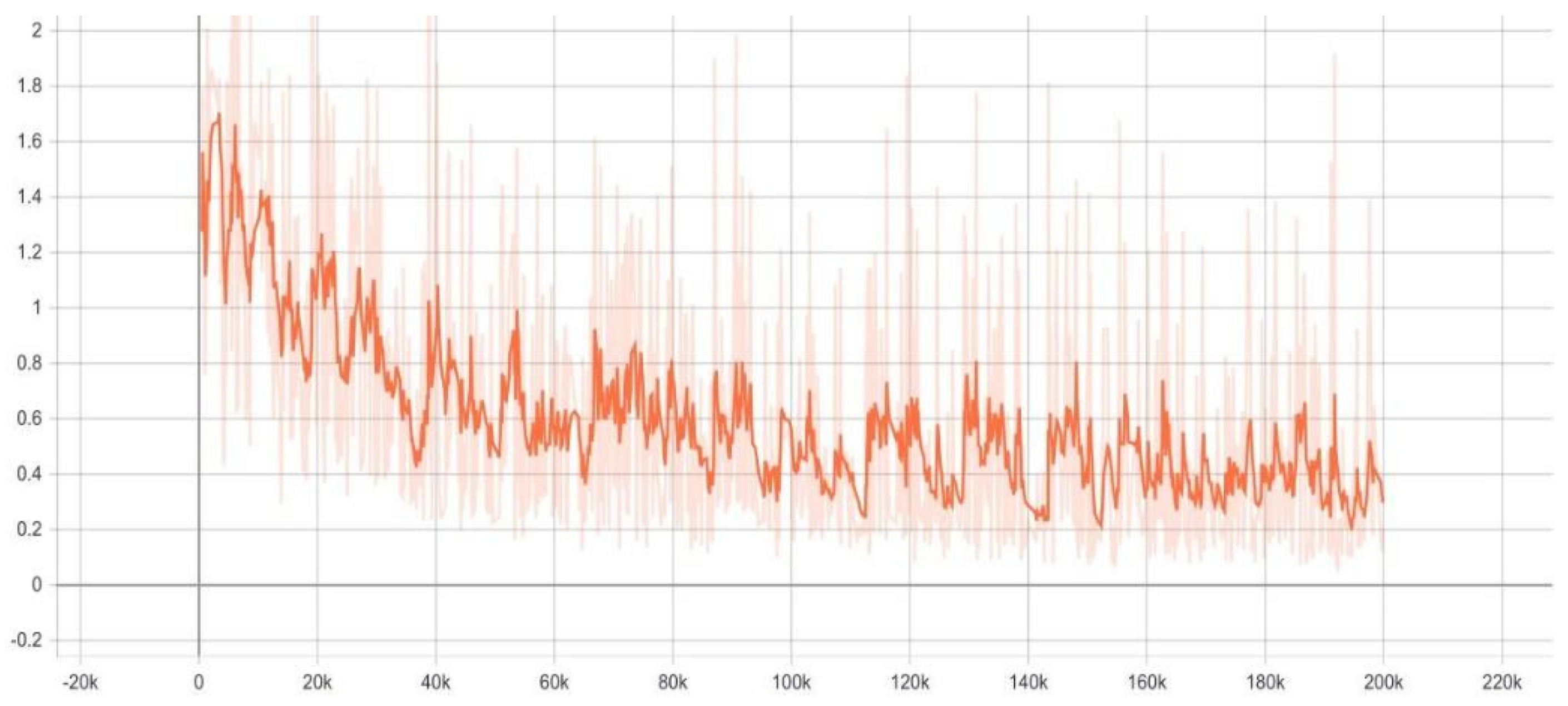
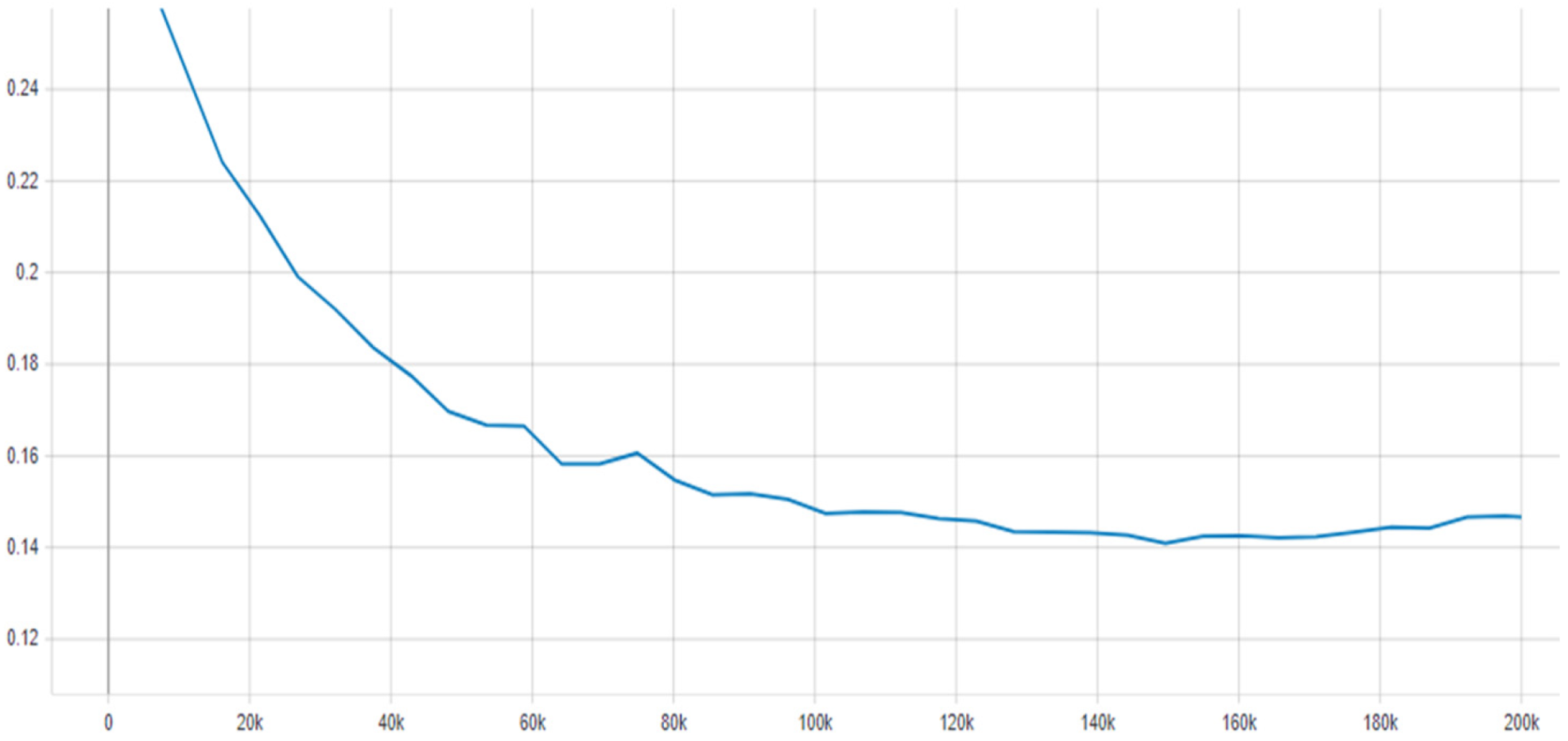
4.1. Training

Tensorboard is a powerful visualization tool for evaluating model performances. It was utilized in this work for obtaining the graphs and analyzing purposes. We consider COCO mAP at [0.5:0.95] IOU and mAP at a 0.5 IOU threshold to evaluate the model’s performance.

4.1.1. Case 1: Configuration 1

In this case, we considered learning rate configuration 1. With that configuration, the Faster R-CNN inceptionv2 COCO model was trained and fine-tuned up to 200 k steps. The model performed considerably well and reached a maximum overall mAP [0.5:0.95]IOU of 30.94% at 149.6 k step (Figure 18). The maximum mAP at the 0.5 IOU threshold was 61.5% at 149.6 k (Figure 19). At the 200 k step, the maximum overall mAP[0.5:0.95]IOU was reached, at 30.57%. The maximum mAP at the 0.5 IOU threshold was 61.29%. These values were considered suitable given the comparatively less amount of data that the model was trained with. The graphs corresponding to the model performance are shown in the following figures. Graphs were generated at a smoothing value of 0.6 to show the overall trend of the training and evaluation process.

Steps on X-axis: One gradient update is considered as a training or evaluation step (iteration). It represents the number of batch-size images that are processed during a single iteration. For instance, we considered 200 images, and our batch size is set to 1 image in training configuration. That means one image was processed during one step, and gradients were updated once. Now the model takes 200 steps to complete the processing of the entire dataset. As the model processed the entire dataset, we say the model completed one epoch.

Y-axis: Y-axis in the following graphs corresponds to their respective losses and mAP of the model.

By observing Figure 20 and Figure 21 for training and evaluation loss, we say the model is performing better as the two loss learning curves show a decreasing trend without huge variations. The X-axis represents the number of training and evaluation steps the model was trained with, while the Y-axis represents the training and evaluation loss recorded at each step respectively. Approximately at 150 k step, the model’s total evaluation loss had reached a minimum of 0.61, and from after that, we observe a very slight increase in the loss values, this indicates the model was trying to overfit slowly and indicates it may not be feasible to train further. The training was stopped at 200 k, and the nearest checkpoint recorded at 200 k step was exported and inferencing was done. This performance was cross-verified with the pre-trained configuration, as it stated at 200 k steps were enough for the model to perform better. Although the model performed quite well on the new unknown images, there was scope in the optimization of the model by tuning the model’s hyperparameters.

One of the observations from the analysis and experiments was: If the data considered was very low, data augmentation techniques such as flipping the images can help increase the mAP. The transfer learning technique was evaluated and justified that it can be quite helpful and quick when training on a new classification task instead of training the network from scratch or initializing with random weights. Hyperparameters such as the learning rate can be tuned further to increase mAP. Having high graphical processing units and performing a grid search or random search method can help us find optimal hyperparameters, but the process may be computationally expensive and time-consuming.

In order to establish fully the notion that our model was finely well-tuned, the losses for the RPN network and the final classifier were also considered. By observing Figure 22 and Figure 23, the decreasing trend of the box classifier classification and localization loss indicates that the final classifier is good at classifying and localizing the detected plant and weed objects. In Figure 22 and Figure 23, X-axis represents the number of evaluation steps and Y-axis represents the classification loss and localization loss recorded at each step respectively.

The final ground truths and detections of various sizes of weeds and plants at the 200 k evaluation step are presented in Figure 24, Figure 25 and Figure 26 corresponding to common dandelion (weed), garden cress and radish respectively. It is worth noticing the model gave predictions with good detection scores.

4.1.2. Case 2: Configuration 2

In this case, we considered learning rate configuration 2. With this configuration, the training process was faster and achieved higher mAP values. With a lesser amount of steps in this configuration, the results obtained were not comparatively better than the results of the learning rate configuration 1. However, the model was overfitting and trying to memorize when trained for a longer time. It was one of the reasons the model achieved a higher overall mAP of 34.82% at (0.5:0.95) IOU (Figure 27) and mAP of 63% at 0.5 IOU threshold at 200 k step (Figure 28). The resultant graphs during the training and evaluation process are shown below. The graphs were generated at a smoothing value of 0.6 for showing the overall trend of the training and evaluation process.

By observing the loss curves in Figure 29 and Figure 30, the localization loss is increasing after the 60 k step. Ideally, all the loss curves should be in decreasing trend, and any large deviations of any loss are considered not suitable for generalization. Considering that, in this case, we should stop training at this point. Hence we can say the chosen learning rate hyperparameter may not be ideal for inferencing purposes compared to case 1 results. With that, case 1 results were considered for inferencing purposes, and the results are reported discussed in the following section.

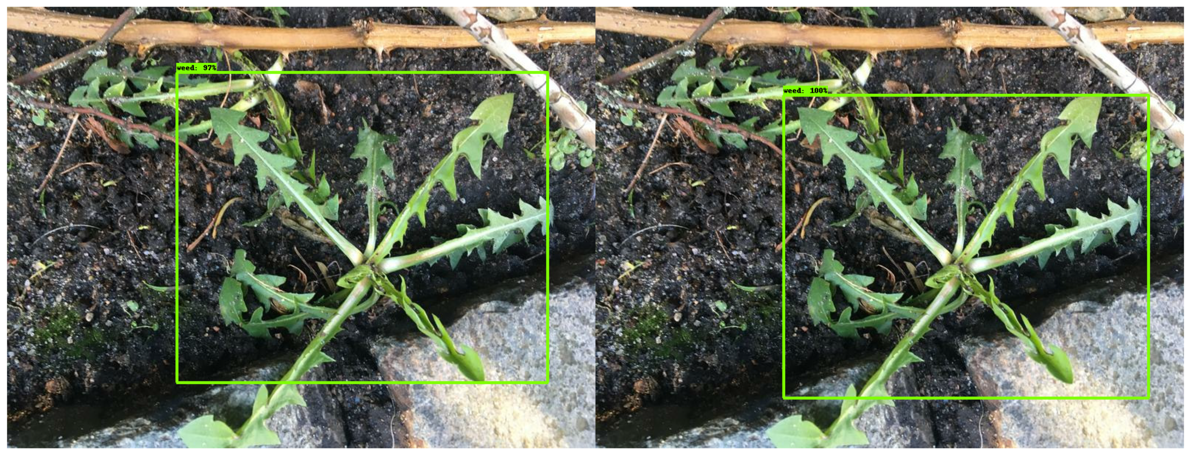
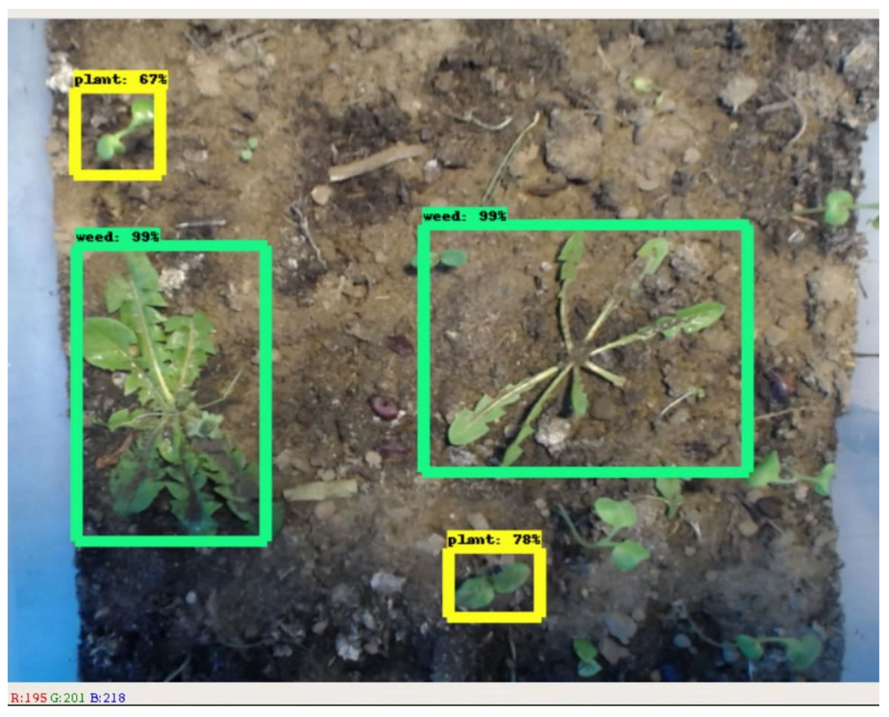
4.2. Plant and Weed Identification

After the model was trained, it was used for inference on real-time data for plant and weed identification. For inferencing a new set of images, the model was saved and exported. For exporting the frozen graph, TensorFlow object detection API’s inbuilt “export inference graph.py” script was used. The python script was modified accordingly to our task. The same training hardware setup and a Logitech stereo camera were used for real-time identification of plants and weeds. A completely new set of images was provided for predictions. The predicted output images are shown in Figure 31, Figure 32 and Figure 33.

4.3. Extracted Stem Positions

With the previously described stem estimation technique, we tested our method in real-time. We observed that the estimated stem positions were close enough (83–97%) to the original stem positions of the weed. The result of the extracted stem position in the image frame is presented in Figure 34.

4.4. Discussion of Results

The use of convolutional neural network-based models has been reported in different areas of agriculture, including disease identification, classification on the basis of ripeness of fruits, plant recognition using leaf images, and identification of weeds [35,101,102,103,104]. The application of convolutional neural networks (CNNs) using the transfer learning technique has also been reported in recent literature in the case of crop/fruit (age) classification. Perez-Perez et al. (2021) reported accuracy of 99.32% in the case of identification of different ripening stages of Medjoul dates [35]. This specific work points to the possibility of tuning the hyperparameters to achieve higher performance parameters with the proposed weeding robot as has been mentioned regarding the results of the current study. In recent years other studies have reported classification of plants through plant and leaf image recognition using convolution neural networks with accuracies up to 99% [103,104]. Sladojevic et al. (2016) reported the use of CNNs for disease recognition by leaf image classification with precision up to 98% [102].

With respect to the classification of different plant species, with the aim of site-specific weed management, Dyrmann et al. (2016) trained a CNN on a set of 10,413 images of 22 different plant species and were able to achieve a classification accuracy of up to 86% [101]. In the reported study, although the number of species classified was high, the images that were considered in the dataset were of plants at the same growth stage i.e., the seedling stage [101]. This makes the classification easier due to the same plant and leaf structure and hence higher accuracies are expected. However, in the case of weed removal applications, multiple weeding procedures might be needed at different times during a crop season, hence training a neural network with images of plants and weeds at different growth stages was done in the current study. The methodology is also reported in a recent study reported in literature where a crop field at two different growth stages was used to train the neural network, achieving an accuracy of 99.48% [105]. The classification accuracies achieved in the current study hence fall in the range of accuracies found in various studies reported in recent literature. The current study adds further value to the research by reporting the mean Average Precision (mAP) of the object detection tasks performed by the trained model. The mAP is an important metric to evaluate object detection models including both classification and localization tasks.

Table 2. Comparison of studies with reported training of CNNs for plant classification and identification tasks.

Reference	Number of Species	Growth Stages	Number of Images (Dataset)	Highest Classification Accuracy	Object Detection: Mean Average Precision (mAP)
Perez-Perez et al. (2021)	1	Ripe and Unripe	1002	99.32%	n.a.
Dyrmann et al. (2016)	22	Seedling	10,413	86.2%	n.a.
Asad and Bais (2020)	2	Two	906	99.48%	n.a.
Current study	3	Multiple	200	Plant: 95% Weed: 99%	31%

gives an overview of three other studies on CNNs for plant/weed/fruit classification that have reported comparable results together with the current study.

5. Conclusions

The weed identifier robot is proposed as a non-chemical solution to the rampant problem of weed infestation in food crop farming systems. Research and implementation of a plant and weed identification system using deep learning and state-of-the-art object detection methods was done. Transfer learning technique was explored and the deep learning model was further analysed, evaluated and justified for better generalization. It was seen that deep learning architectures are much better than conventional machine learning architectures in terms of image identification and predictive performance. A simple unique stem estimation technique was proposed which extracted their positions in the image frame. Consequently, the paper also offers a high-level hardware and software design architecture proposal of a cost-effective autonomous weeding robot.

The developed plant and weed identification system was presented and tested on the real-world data and good confidence scores on classification and identification were achieved. It can be concluded that higher values of mAP could be achieved with more steps with the right hyperparameters. Real-time identification was done using a Logitech web camera and it was observed that the model was good at identifying and distinguishing between plants and weeds. The stem position estimation approach was tested and it was found that accuracies were directly dependent on the bounding box localization during identification. Based on our observation, we conclude that this technique also reduces the amount of computation when compared with other methods. In addition to building the prototype and validation studies, future work in this direction could include investigations on choosing a method to find the right hyperparameters for optimization of the identification function of the robot. Further studies could explore 3D position estimation methods to determine the position from the center of the identified weed in the 2D image frame to the real-world robot frame.

References

1. Varma, P. Adoption of System of Rice Intensification under Information Constraints: An Analysis for India. J. Dev. Stud. 2018, 54, 1838–1857. [Google Scholar] [CrossRef]
2. Delmotte, S.; Tittonell, P.; Mouret, J.-C.; Hammond, R.; Lopez-Ridaura, S. On farm assessment of rice yield variability and productivity gaps between organic and conventional cropping systems under Mediterranean climate. Eur. J. Agron. 2011, 35, 223–236. [Google Scholar] [CrossRef]
3. Shennan, C.; Krupnik, T.J.; Baird, G.; Cohen, H.; Forbush, K.; Lovell, R.J.; Olimpi, E.M. Organic and Conventional Agriculture: A Useful Framing? Annu. Rev. Environ. Resour. 2017, 42, 317–346. [Google Scholar] [CrossRef]
4. John, A.; Fielding, M. Rice production constraints and “new” challenges for South Asian smallholders: Insights into de facto research priorities. Agric. Food Secur. 2014, 3, 1–16. [Google Scholar] [CrossRef] [Green Version]
5. Hazra, K.K.; Swain, D.K.; Bohra, A.; Singh, S.S.; Kumar, N.; Nath, C.P. Organic rice: Potential production strategies, challenges and prospects. Org. Agric. 2018, 8, 39–56. [Google Scholar] [CrossRef]
6. Sujaritha, M.; Annadurai, S.; Satheeshkumar, J.; Kowshik Sharan, S.; Mahesh, L. Weed detecting robot in sugarcane fields using fuzzy real time classifier. Comput. Electron. Agric. 2017, 134, 160–171. [Google Scholar] [CrossRef]
7. Zahm, S.H.; Ward, M.H. Pesticides and childhood cancer. Environ. Health Perspect. 1998, 106, 893–908. [Google Scholar] [CrossRef]
8. Chitra, G.A.; Muraleedharan, V.R.; Swaminathan, T.; Veeraraghavan, D. Use of pesticides and its impact on health of farmers in south India. Int. J. Occup. Environ. Health 2006, 12, 228–233. [Google Scholar] [CrossRef]
9. Wilson, C. Environmental and human costs of commercial agricultural production in South Asia. Int. J. Soc. Econ. 2000, 27, 816–846. [Google Scholar] [CrossRef] [Green Version]
10. Uphoff, N. SRI: An agroecological strategy to meet multiple objectives with reduced reliance on inputs. Agroecol. Sustain. Food Syst. 2017, 41, 825–854. [Google Scholar] [CrossRef]
11. Wayayok, A.; Soom, M.A.M.; Abdan, K.; Mohammed, U. Impact of Mulch on Weed Infestation in System of Rice Intensification (SRI) Farming. Agric. Agric. Sci. Procedia 2014, 2, 353–360. [Google Scholar] [CrossRef] [Green Version]
12. Krupnik, T.J.; Rodenburg, J.; Haden, V.R.; Mbaye, D.; Shennan, C. Genotypic trade-offs between water productivity and weed competition under the System of Rice Intensification in the Sahel. Agric. Water Manag. 2012, 115, 156–166. [Google Scholar] [CrossRef]
13. RCEP. Royal Commission for Environmental Pollution 1979 Seventh Report. Agriculture and Pollution; RCEP: London, UK, 1979. [Google Scholar]
14. Moss, B. Water pollution by agriculture. Philos. Trans. R. Soc. B Biol. Sci. 2008, 363, 659–666. [Google Scholar] [CrossRef] [PubMed] [Green Version]
15. James, C.; Fisher, J.; Russell, V.; Collings, S.; Moss, B. Nitrate availability and hydrophyte species richness in shallow lakes. Freshw. Biol. 2005, 50, 1049–1063. [Google Scholar] [CrossRef]
16. Mehaffey, M.H.; Nash, M.S.; Wade, T.G.; Ebert, D.W.; Jones, K.B.; Rager, A. Linking land cover and water quality in New York City’s water supply watersheds. Environ. Monit. Assess. 2005, 107, 29–44. [Google Scholar] [CrossRef]
17. Sala, O.E.; Chapin, F.S.; Armesto, J.J.; Berlow, E.; Bloomfield, J.; Dirzo, R.; Huber-Sanwald, E.; Huenneke, L.F.; Jackson, R.B.; Kinzig, A.; et al. Global biodiversity scenarios for the year 2100. Science 2000, 287, 1770–1774. [Google Scholar] [CrossRef]
18. Pimentel, D.; Pimentel, M. Comment: Adverse environmental consequences of the Green Revolution. In Resources, Environment and Population-Present Knowledge, Future Options, Population and Development Review; Davis, K., Bernstam, M., Eds.; Oxford University Press: Oxford, UK, 1991. [Google Scholar]
19. Pimentel, D.; Acquay, H.; Biltonen, M.; Rice, P.; Silva, M.; Nelson, J.; Lipner, V.; Horowitz, A.; Amore, M.D. Environmental and Economic Costs of Pesticide Use. Am. Inst. Biol. Sci. 1992, 42, 750–760. [Google Scholar] [CrossRef]
20. Orlando, F.; Alali, S.; Vaglia, V.; Pagliarino, E.; Bacenetti, J.; Bocchi, S.; Bocchi, S. Participatory approach for developing knowledge on organic rice farming: Management strategies and productive performance. Agric. Syst. 2020, 178, 102739. [Google Scholar] [CrossRef]
21. Barker, R.; Herdt, R.W.; Rose, H. The Rice Economy of Asia; The Johns Hopkins University Press: Baltimore, MD, USA, 1985. [Google Scholar]
22. FAO. FAO Production Yearbooks (1961–1988); FAO Statistics Series; FAO: Rome, Italy, 1988. [Google Scholar]
23. Chen, Z.; Shah, T.M. An Introduction to the Global Soil Status; RUVIVAL Publication Series; Schaldach, R., Otterpohl, R., Eds.; Hamburg University of Technology: Hamburg, Germany, 2019; Volume 5, pp. 7–17. [Google Scholar]
24. Kopittke, P.M.; Menzies, N.W.; Wang, P.; McKenna, B.A.; Lombi, E. Soil and the intensification of agriculture for global food security. Environ. Int. 2019, 132, 105078. [Google Scholar] [CrossRef]
25. Nawaz, A.; Farooq, M. Weed management in resource conservation production systems in Pakistan. Crop Prot. 2016, 85, 89–103. [Google Scholar] [CrossRef]
26. Sreekanth, M.; Hakeem, A.H.; Peer, Q.J.A.; Rashid, I.; Farooq, F. Adoption of Recommended Package of Practices by Rice Growers in District Baramulla. J. Appl. Nat. Sci. 2019, 11, 188–192. [Google Scholar] [CrossRef]
27. Holt-Giménez, E.; Altieri, M.A. Agroecology, food sovereignty, and the new green revolution. Agroecol. Sustain. Food Syst. 2013, 37, 90–102. [Google Scholar] [CrossRef]
28. Wezel, A.; Bellon, S.; Doré, T.; Francis, C.; Vallod, D.; David, C. Agroecology as a science, a movement and a practice. A review. Agron. Sustain. Dev. 2009, 29, 503–515. [Google Scholar] [CrossRef] [Green Version]
29. Bajwa, A.A.; Mahajan, G.; Chauhan, B.S. Nonconventional weed management strategies for modern agriculture. Weed Sci. 2015, 63, 723–747. [Google Scholar] [CrossRef]
30. Zhang, C.; Kovacs, J.M. The application of small unmanned aerial systems for precision agriculture: A review. Precis. Agric. 2012, 13, 693–712. [Google Scholar] [CrossRef]
31. Lamb, D.W.; Weedon, M. Evaluating the accuracy of mapping weeds in fallow fields using airborne digital imaging: Panicum effusum in oilseed rape stubble. Weed Res. 1998, 38, 443–451. [Google Scholar] [CrossRef]
32. Medlin, C.R.; Shaw, D.R. Economic comparison of broadcast and site-specific herbicide applications in nontransgenic and glyphosate-tolerant Glycine max. Weed Sci. 2000, 48, 653–661. [Google Scholar] [CrossRef]
33. Huang, Y.; Reddy, K.N.; Fletcher, R.S.; Pennington, D. UAV low-altitude remote sensing for precision weed management. Weed Technol. 2018, 32, 2–6. [Google Scholar] [CrossRef]
34. Freeman, P.K.; Freeland, R.S. Agricultural UAVs in the US: Potential, policy, and hype. Remote Sens. Appl. Soc. Environ. 2015, 2, 35–43. [Google Scholar]
35. Pérez-Pérez, B.D.; García Vázquez, J.P.; Salomón-Torres, R. Evaluation of Convolutional Neural Networks’ Hyperparameters with Transfer Learning to Determine Sorting of Ripe Medjool Dates. Agriculture 2021, 11, 115. [Google Scholar] [CrossRef]
36. Graeub, B.E.; Chappell, M.J.; Wittman, H.; Ledermann, S.; Kerr, R.B.; Gemmill-Herren, B. The State of Family Farms in the World. World Dev. 2016, 87, 1–15. [Google Scholar] [CrossRef] [Green Version]
37. Wezel, A.; Casagrande, M.; Celette, F.; Vian, J.F.; Ferrer, A.; Peigné, J. Agroecological practices for sustainable agriculture. A review. Agron. Sustain. Dev. 2014, 34, 1–20. [Google Scholar] [CrossRef] [Green Version]
38. Harker, K.N.; O’Donovan, J.T. Recent Weed Control, Weed Management, and Integrated Weed Management. Weed Technol. 2013, 27, 1–11. [Google Scholar] [CrossRef]
39. Melander, B.; Rasmussen, I.A.; Bàrberi, P. Integrating physical and cultural methods of weed control—Examples from European research. Weed Sci. 2005, 53, 369–381. [Google Scholar] [CrossRef]
40. Benbrook, C.M. Trends in glyphosate herbicide use in the United States and globally. Environ. Sci. Eur. 2016, 28, 3. [Google Scholar] [CrossRef] [PubMed] [Green Version]
41. Helander, M.; Saloniemi, I.; Saikkonen, K. Glyphosate in northern ecosystems. Trends Plant Sci. 2012, 17, 569–574. [Google Scholar] [CrossRef]
42. IARC. IARC Monographs Volume 112: Evaluation of Five Organophosphate Insecticides and Herbicides; IARC: Lyon, France, 2017. [Google Scholar]
43. Jayasumana, C.; Paranagama, P.; Agampodi, S.; Wijewardane, C.; Gunatilake, S.; Siribaddana, S. Drinking well water and occupational exposure to Herbicides is associated with chronic kidney disease, in Padavi-Sripura, Sri Lanka. Environ. Health 2015, 14, 6. [Google Scholar] [CrossRef] [Green Version]
44. Monarch Butterfles: The Problem with Herbicides. Available online: https://www.sciencedaily.com/releases/2017/05/170517143600.htm (accessed on 23 January 2021).
45. Motta, E.V.S.; Raymann, K.; Moran, N.A. Glyphosate perturbs the gut microbiota of honey bees. Proc. Natl. Acad. Sci. USA 2018, 115, 10305–10310. [Google Scholar] [CrossRef] [Green Version]
46. Kanissery, R.; Gairhe, B.; Kadyampakeni, D.; Batuman, O.; Alferez, F. Glyphosate: Its environmental persistence and impact on crop health and nutrition. Plants 2019, 8, 499. [Google Scholar] [CrossRef] [PubMed] [Green Version]
47. Murphy, K.P. Machine Learning: A Probabilistic Perspective; MIT Press: Cambridge, MA, USA, 2012; ISBN 978-0-262-01802-9. [Google Scholar]
48. Goodfellow, I.; Bengio, Y.; Courville, A. Deep Learning; MIT Press: Cambridge, MA, USA, 2016; ISBN 978-0262035613. [Google Scholar]
49. Brownlee, J. What Is Deep Learning? Available online: https://machinelearningmastery.com/what-is-deep-learning/ (accessed on 23 January 2021).
50. Liakos, K.; Busato, P.; Moshou, D.; Pearson, S.; Bochtis, D. Machine Learning in Agriculture: A Review. Sensors 2018, 18, 2674. [Google Scholar] [CrossRef] [Green Version]
51. Mohanty, S.P.; Hughes, D.P.; Salathé, M. Using deep learning for image-based plant disease detection. Front. Plant Sci. 2016, 7, 1–10. [Google Scholar] [CrossRef] [PubMed] [Green Version]
52. Narayanasamy, P. Biological Management of Diseases of Crops; Springer: Dordrecht, The Netherlands, 2013; ISBN 978-94-007-6379-1. [Google Scholar]
53. Saleem, M.H.; Potgieter, J.; Arif, K.M. Mahmood Arif Plant Disease Detection and Classification by Deep Learning. Plants 2019, 8, 468. [Google Scholar] [CrossRef] [PubMed] [Green Version]
54. Fuentes, A.; Yoon, S.; Kim, S.; Park, D. A Robust Deep-Learning-Based Detector for Real-Time Tomato Plant Diseases and Pests Recognition. Sensors 2017, 17, 2022. [Google Scholar] [CrossRef] [PubMed] [Green Version]
55. Raun, W.R.; Solie, J.B.; Johnson, G.V.; Stone, M.L.; Lukina, E.V.; Thomason, W.E.; Schepers, J.S. In-season prediction of potential grain yield in winter wheat using canopy reflectance. Agron. J. 2001, 93, 131–138. [Google Scholar] [CrossRef] [Green Version]
56. Filippi, P.; Jones, E.J.; Wimalathunge, N.S.; Somarathna, P.D.S.N.; Pozza, L.E.; Ugbaje, S.U.; Jephcott, T.G.; Paterson, S.E.; Whelan, B.M.; Bishop, T.F.A. An approach to forecast grain crop yield using multi-layered, multi-farm data sets and machine learning. Precis. Agric. 2019, 20, 1015–1029. [Google Scholar] [CrossRef]
57. Ashapure, A.; Oh, S.; Marconi, T.G.; Chang, A.; Jung, J.; Landivar, J.; Enciso, J. Unmanned aerial system based tomato yield estimation using machine learning. In Proceedings Volume 11008, Autonomous Air and Ground Sensing Systems for Agricultural Optimization and Phenotyping IV; SPIE: Baltimore, MD, USA, 2019; p. 22. [Google Scholar] [CrossRef]
58. Khaki, S.; Wang, L.; Archontoulis, S.V. A CNN-RNN Framework for Crop Yield Prediction. Front. Plant Sci. 2020, 10, 1–14. [Google Scholar] [CrossRef]
59. Russello, H. Convolutional Neural Networks for Crop Yield Prediction Using Satellite Images. Master’s Thesis, University of Amsterdam, Amsterdam, The Netherland, 2018. [Google Scholar]
60. Sun, Y.; Liu, Y.; Wang, G.; Zhang, H. Deep Learning for Plant Identification in Natural Environment. Comput. Intell. Neurosci. 2017, 2017, 1–6. [Google Scholar] [CrossRef]
61. Du, J.-X.; Wang, X.-F.; Zhang, G.-J. Leaf shape based plant species recognition. Appl. Math. Comput. 2007, 185, 883–893. [Google Scholar] [CrossRef]
62. Grinblat, G.L.; Uzal, L.C.; Larese, M.G.; Granitto, P.M. Deep learning for plant identification using vein morphological patterns. Comput. Electron. Agric. 2016, 127, 418–424. [Google Scholar] [CrossRef] [Green Version]
63. Wu, S.G.; Bao, F.S.; Xu, E.Y.; Wang, Y.-X.; Chang, Y.-F.; Xiang, Q.-L. A Leaf Recognition Algorithm for Plant Classification Using Probabilistic Neural Network. In Proceedings of the 2007 IEEE International Symposium on Signal Processing and Information Technology, Giza, Egypt, 15–18 December 2007; pp. 11–16. [Google Scholar] [CrossRef] [Green Version]
64. Goëau, H.; Bonnet, P.; Baki, V.; Barbe, J.; Amap, U.M.R.; Carré, J.; Barthélémy, D. Pl@ntNet Mobile App. In Proceedings of the 21st ACM international conference on Multimedia, Barcelona, Spain, 21–25 October 2013; pp. 423–424. [Google Scholar]
65. Wäldchen, J.; Mäder, P. Machine learning for image based species identification. Methods Ecol. Evol. 2018, 9, 2216–2225. [Google Scholar] [CrossRef]
66. Liebman, M.; Baraibar, B.; Buckley, Y.; Childs, D.; Christensen, S.; Cousens, R.; Eizenberg, H.; Heijting, S.; Loddo, D.; Merotto, A.; et al. Ecologically sustainable weed management: How do we get from proof-of-concept to adoption? Ecol. Appl. 2016, 26, 1352–1369. [Google Scholar] [CrossRef]
67. Farooq, A.; Jia, X.; Hu, J.; Zhou, J. Knowledge Transfer via Convolution Neural Networks for Multi-Resolution Lawn Weed Classification. In Proceedings of the 2019 10th Workshop on Hyperspectral Imaging and Signal Processing: Evolution in Remote Sensing (WHISPERS), Amsterdam, The Netherlands, 24–26 September 2019; Volume 2019. [Google Scholar]
68. Dadashzadeh, M.; Abbaspour, G.Y.; Mesri, G.T.; Sabzi, S.; Hernandez-Hernandez, J.L.; Hernandez-Hernandez, M.; Arribas, J.I. Weed Classification for Site-Specific Weed. Plants 2020, 9, 559. [Google Scholar] [CrossRef]
69. Ashqar, B.A.; Abu-Nasser, B.S.; Abu-Naser, S.S. Plant Seedlings Classification Using Deep Learning. Int. J. Acad. Inf. Syst. Res. 2019, 46, 745–749. [Google Scholar]
70. Smith, L.N.; Byrne, A.; Hansen, M.F.; Zhang, W.; Smith, M.L. Weed classification in grasslands using convolutional neural networks. Int. Soc. Opt. Photonics 2019, 11139, 1113919. [Google Scholar] [CrossRef]
71. Simon, H. Neural Networks: A Comprehensive Foundation; McMaster University: Hamilton, ON, Canada, 2005; p. 823. [Google Scholar]
72. Park, S.H. Artificial Intelligence in Medicine: Beginner’s Guide. J. Korena Soc Radiol. 2018, 78, 301–308. [Google Scholar] [CrossRef]
73. Chollet, F. Deep Learning with Python; Manning: New York, NY, USA, 2018; Volume 361. [Google Scholar]
74. Convolutional Neural Networks (CNNs/ConvNets). Available online: https://cs231n.github.io/convolutional-networks/ (accessed on 23 January 2021).
75. Brownlee, J. A Gentle Introduction to Object Recognition with Deep Learning. Available online: https://machinelearningmastery.com/object-recognition-with-deep-learning/ (accessed on 23 January 2021).
76. Ren, S.; He, K.; Girshick, R.; Sun, J. Faster R-CNN: Towards Real-Time Object Detection with Region Proposal Networks. IEEE Trans. Pattern Anal. Mach. Intell. 2017, 39, 1137–1149. [Google Scholar] [CrossRef] [PubMed] [Green Version]
77. Girshick, R. Fast r-cnn. In Proceedings of the IEEE International Conference on Computer Vision, Santiago, Chile, 11–18 December 2015; pp. 1440–1448. [Google Scholar]
78. He, K.; Gkioxari, G.; Dollár, P.; Girshick, R. Mask R-CNN. IEEE Trans. Pattern Anal. Mach. Intell. 2020, 42, 386–397. [Google Scholar] [CrossRef]
79. Liu, W.; Anguelov, D.; Erhan, D.; Szegedy, C.; Reed, S.; Fu, C.-Y.; Berg, A.C. SSD: Single Shot MultiBox Detector. In ECCV 2016: Computer Vision–ECCV 2016; Lecture Notes in Computer Science; Springer: Cham, Germany, 2016; Volume 9905, pp. 21–37. ISBN 9783319464473. [Google Scholar] [CrossRef] [Green Version]
80. Redmon, J.; Divvala, S.; Girshick, R.; Farhadi, A. You Only Look Once: Unified, Real-Time Object Detection. In Proceedings of the 2016 IEEE Conference on Computer Vision and Pattern Recognition (CVPR), Las Vegas, NV, USA, 27–30 June 2016; Volume 2016, pp. 779–788. [Google Scholar]
81. Girshick, R.; Donahue, J.; Darrell, T.; Malik, J. Rich feature hierarchies for accurate object detection and semantic segmentation. In Proceedings of the IEEE Conference on Computer Vision and Pattern Recognition, Columbus, OH, USA, 23–28 June 2014; pp. 580–587. [Google Scholar]
82. Weng, L. Object Detection for Dummies Part 3: R-CNN Family. Available online: https://lilianweng.github.io/lil-log/2017/12/31/object-recognition-for-dummies-part-3.html (accessed on 23 January 2021).
83. Olivas, E.S.; Guerrero, J.D.M.; Martinez-Sober, M.; Magdalena-Benedito, J.R.; Serrano, L. Handbook of Research on machine Learning Applications and Trends: Algorithms, Methods, and Techniques; IGI Global: Hershey, PA, USA, 2009; ISBN 1605667676. [Google Scholar]
84. Kaya, A.; Keceli, A.S.; Catal, C.; Yalic, H.Y.; Temucin, H.; Tekinerdogan, B. Analysis of transfer learning for deep neural network based plant classification models. Comput. Electron. Agric. 2019, 158, 20–29. [Google Scholar] [CrossRef]
85. Williams, J.; Tadesse, A.; Sam, T.; Sun, H.; Montanez, G.D. Limits of Transfer Learning. In Proceedings of the International Conference on Machine Learning, Optimization, and Data Science, Siena, Italy, 19–23 July 2020; Springer: Berlin/Heidelberg, Germany, 2020; pp. 382–393. [Google Scholar]
86. Pan, S.J.; Yang, Q. A survey on transfer learning. IEEE Trans. Knowl. Data Eng. 2009, 22, 1345–1359. [Google Scholar] [CrossRef]
87. Zhao, W. Research on the deep learning of the small sample data based on transfer learning. AIP Conf. Proc. 2017, 1864, 20018. [Google Scholar]
88. Onshape. Available online: https://www.onshape.com/en/ (accessed on 23 January 2021).
89. Pandilov, Z.; Dukovski, V. Comparison of the characteristics between serial and parallel robots. Acta Tech. Corviniensis-Bull. Eng. 2014, 7, 143. [Google Scholar]
90. Wu, L.; Zhao, R.; Li, Y.; Chen, Y.-H. Optimal Design of Adaptive Robust Control for the Delta Robot with Uncertainty: Fuzzy Set-Based Approach. Appl. Sci. 2020, 10, 3472. [Google Scholar] [CrossRef]
91. Pimentel, D. Environmental and Economic Costs of the Application of Pesticides Primarily in the United States. Environ. Dev. Sustain. 2005, 7, 229–252. [Google Scholar] [CrossRef]
92. Siemens, M.C. Robotic weed control. In Proceedings of the California Weed Science Society, Monterey, CA, USA, 23 June 2014; Volume 66, pp. 76–80. [Google Scholar]
93. Ecorobotix. Available online: https://www.ecorobotix.com/en/autonomous-robot-weeder/ (accessed on 9 February 2021).
94. Pilz, K.H.; Feichter, S. How robots will revolutionize agriculture. In Proceedings of the 2017 European Conference on Educational Robotics, Sofia, Bulgaria, 24–28 April 2017. [Google Scholar]
95. Schnitkey, G. Historic Fertilizer, Seed, and Chemical Costs with 2019 Projections. Farmdoc Daily, 5 June 2018; 102. [Google Scholar]
96. ROS Documentation. Available online: http://wiki.ros.org/Documentation (accessed on 23 January 2021).
97. Raspberry Pi. Available online: https://www.raspberrypi.org/products/ (accessed on 23 January 2021).
98. Coral Dev Board. Available online: https://coral.ai/products/dev-board/ (accessed on 23 January 2021).
99. Embedded Systems for Next-Generation Autonmous Machines. Available online: https://www.nvidia.com/de-de/autonomous-machines/embedded-systems/ (accessed on 23 January 2021).
100. Lottes, P.; Behley, J.; Chebrolu, N.; Milioto, A.; Stachniss, C. Robust joint stem detection and crop-weed classification using image sequences for plant-specific treatment in precision farming. J. F. Robot. 2020, 37, 20–34. [Google Scholar] [CrossRef]
101. Dyrmann, M.; Karstoft, H.; Midtiby, H.S. Plant species classification using deep convolutional neural network. Biosyst. Eng. 2016, 151, 72–80. [Google Scholar] [CrossRef]
102. Sladojevic, S.; Arsenovic, M.; Anderla, A.; Culibrk, D.; Stefanovic, D. Deep Neural Networks Based Recognition of Plant Diseases by Leaf Image Classification. Comput. Intell. Neurosci. 2016, 2016, 3289801. [Google Scholar] [CrossRef] [PubMed] [Green Version]
103. Jeon, W.-S.; Rhee, S.-Y. Plant Leaf Recognition Using a Convolution Neural Network. Int. J. Fuzzy Log. Intell. Syst. 2017, 17, 26–34. [Google Scholar] [CrossRef] [Green Version]
104. Abdullahi, H.S.; Sheriff, R.; Mahieddine, F. Convolution neural network in precision agriculture for plant image recognition and classification. In Proceedings of the 2017 Seventh International Conference on Innovative Computing Technology (INTECH), Luton, UK, 16–18 August 2017; Volume 10. [Google Scholar]
105. Asad, M.H.; Bais, A. Weed detection in canola fields using maximum likelihood classification and deep convolutional neural network. Inf. Process. Agric. 2020, 7, 535–545. [Google Scholar] [CrossRef]
Figure 1. Weeds growing in between rice crop rows (Source: Author).
Agriculture 11 00222 g001
Figure 2. Machine learning approach.
Agriculture 11 00222 g002
Figure 3. A non-linear mathematical model of an artificial neuron [71].
Agriculture 11 00222 g003
Figure 4. A feed-forward neural network [72].
Agriculture 11 00222 g004
Figure 5. A convolutional neural network (CNN) [74].
Agriculture 11 00222 g005
Figure 6. The Region-Based Convolutional Neural Network (R-CNN) family.
Agriculture 11 00222 g006
Figure 7. The transfer learning technique.
Agriculture 11 00222 g007
Figure 8. A rough representation of the idea of the plant and weed classifier robot.
Agriculture 11 00222 g008
Figure 9. A schematic of a delta robot manipulator with three degrees of freedom: (a) A Delta robot with three degrees of freedom; (b) A three-dimensional model of a Delta robot with the different pa-rameters [90].
Agriculture 11 00222 g009
Figure 10. High-level hardware design block diagram for the weeding robot.
Agriculture 11 00222 g010
Figure 11. High-level software block diagram for the weeding robot.
Agriculture 11 00222 g011
Figure 12. Proposed plant and weed identification pipeline.
Agriculture 11 00222 g012
Figure 13. Test weeds: two photographs of common Dandelion that were used in the training.
Agriculture 11 00222 g013
Figure 14. Test plants: A few photographs of Radish seedlings (Left) and Cress (Right) that were used in the training.
Agriculture 11 00222 g014
Figure 15. Annotating weed images using labeling software.
Agriculture 11 00222 g015
Figure 16. Inception module with dimension reduction.
Agriculture 11 00222 g016
Figure 17. Graphical representation of Intersection Over Union (IOU) (Source: Adrian Rosebrock/Creative Commons).
Agriculture 11 00222 g017
Figure 18. Overall mean Average Precision (mAP) at (0.5:0.95) IOU, X-axis: steps, Y-axis: mean average precision.
Agriculture 11 00222 g018
Figure 19. mAP at 0.5 IOU, X-axis: steps, Y-axis: mean average precision.
Agriculture 11 00222 g019
Figure 20. Training loss, X-axis: steps, Y-axis: training loss.
Agriculture 11 00222 g020
Figure 21. Total evaluation loss, X-axis: steps, Y-axis: evaluation loss.
Agriculture 11 00222 g021
Figure 22. BoxClassifier: classification loss, X-axis: steps, Y-axis: classification loss.
Agriculture 11 00222 g022
Figure 23. BoxClassifier: localisation loss, X-axis: steps, Y-axis: localisation loss.
Agriculture 11 00222 g023
Figure 24. Left: detection (97%), Right: groundtruth—larger object.
Agriculture 11 00222 g024
Figure 25. Left: detection (98%), Right: groundtruth—smaller object.
Agriculture 11 00222 g025
Figure 26. Left: detection (88–99%), Right: groundtruth—medium sized object.
Agriculture 11 00222 g026
Figure 27. Overall mAP at (0.5:0.95) IOU, X-axis: steps, Y-axis: mean average precision.
Agriculture 11 00222 g027
Figure 28. mAP at 0.5 IOU, X-axis: steps, Y-axis: mean average precision.
Agriculture 11 00222 g028
Figure 29. Training loss, X-axis: steps, Y-axis: training loss.
Agriculture 11 00222 g029
Figure 30. Total evaluation loss, X-axis: steps, Y-axis: evaluation loss.
Agriculture 11 00222 g030
Figure 31. Plant and weed identification: detection of weed (92%).
Agriculture 11 00222 g031
Figure 32. Plant and weed identification in black soil.
Agriculture 11 00222 g032
Figure 33. Plant and weed identification in brown soil under artificial light.
Agriculture 11 00222 g033
Figure 34. Estimated stem position of the weeds and plants using the trained robot.
Agriculture 11 00222 g034