
A Four Stage Image Processing Algorithm for Detecting and Counting of Bagworm, Metisa plana Walker (Lepidoptera: Psychidae)


Abstract
:1. Introduction
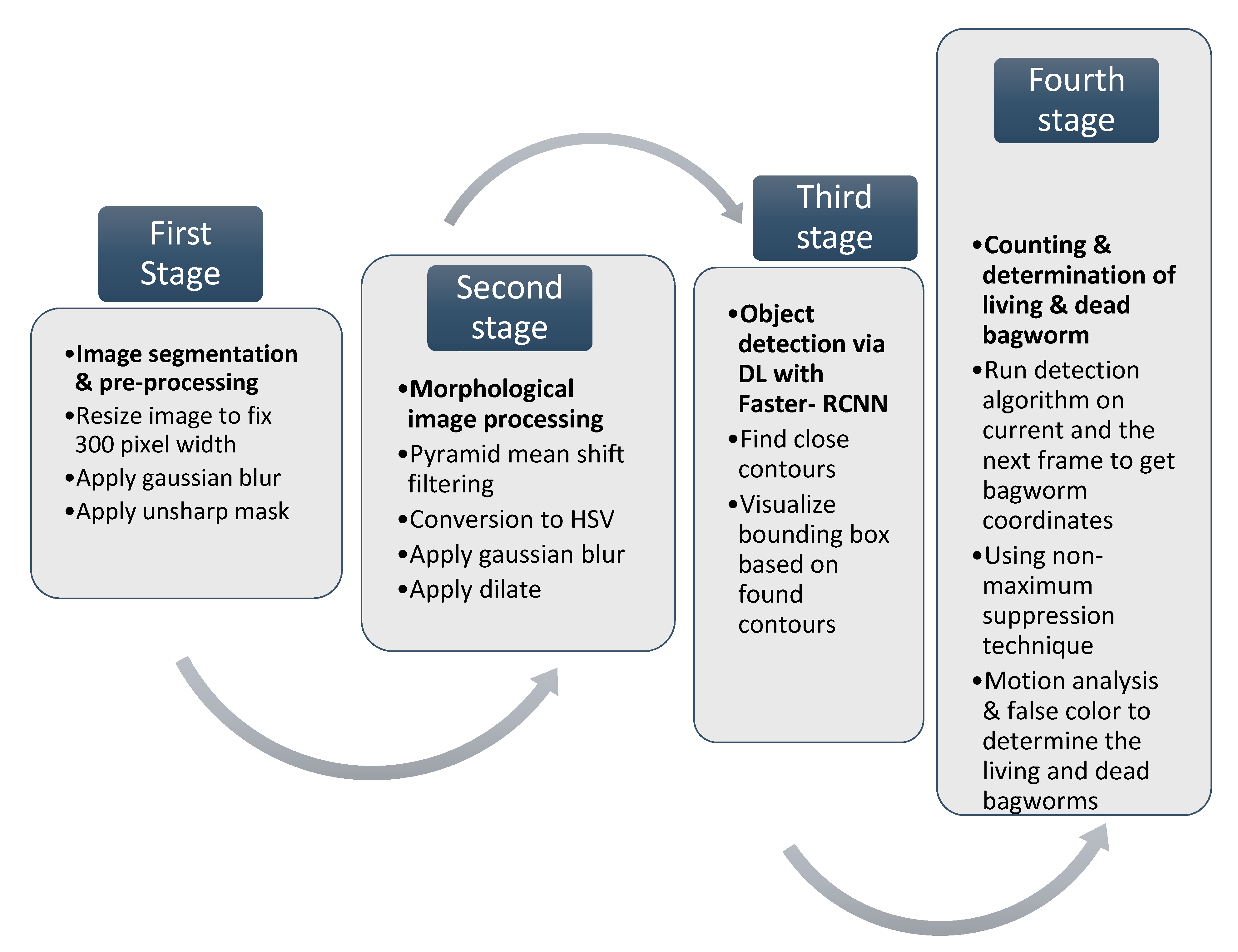
2. Four Stage Methodology for the Bagworm Detection Algorithm
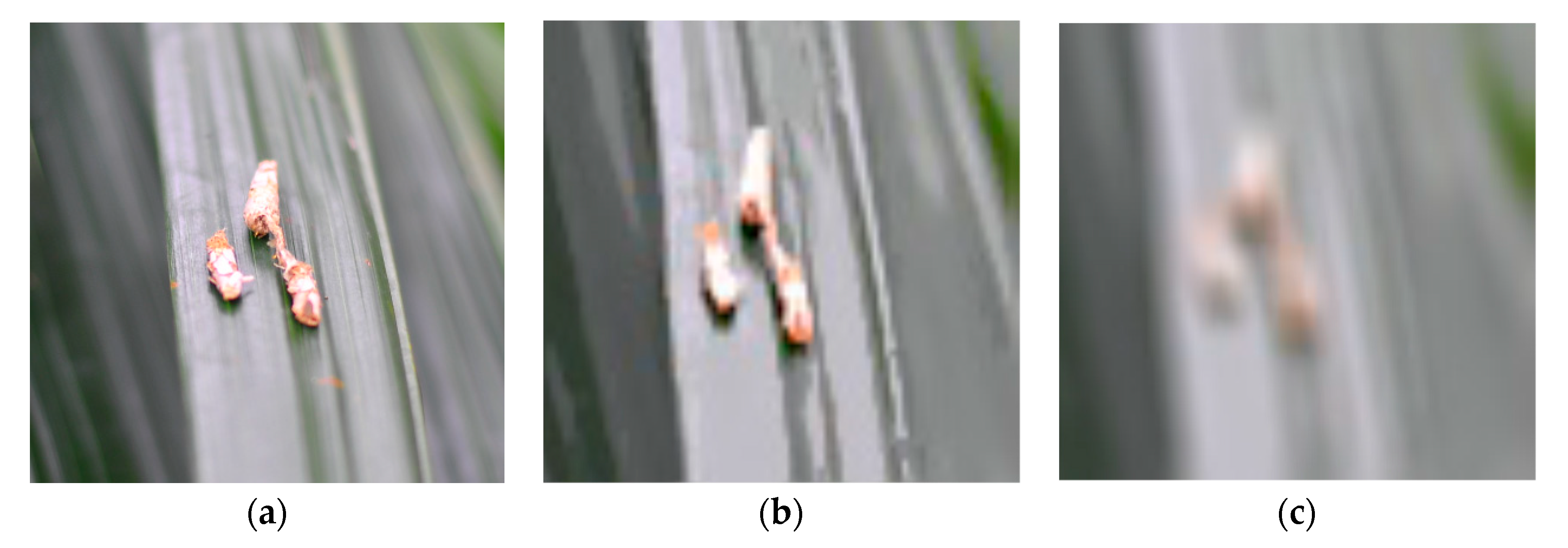
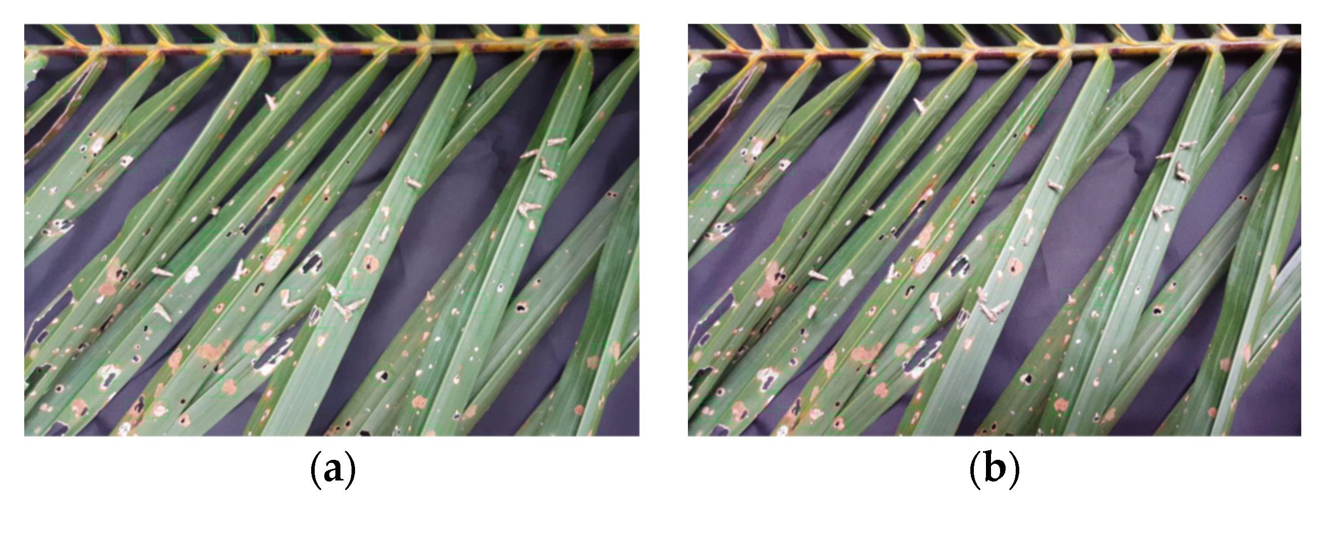
2.1. First Stage—Image Segmentation
2.2. Second Stage—Morphological Image Processing
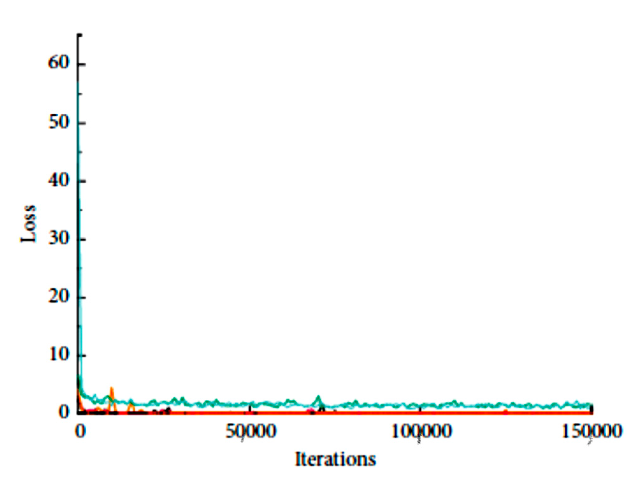
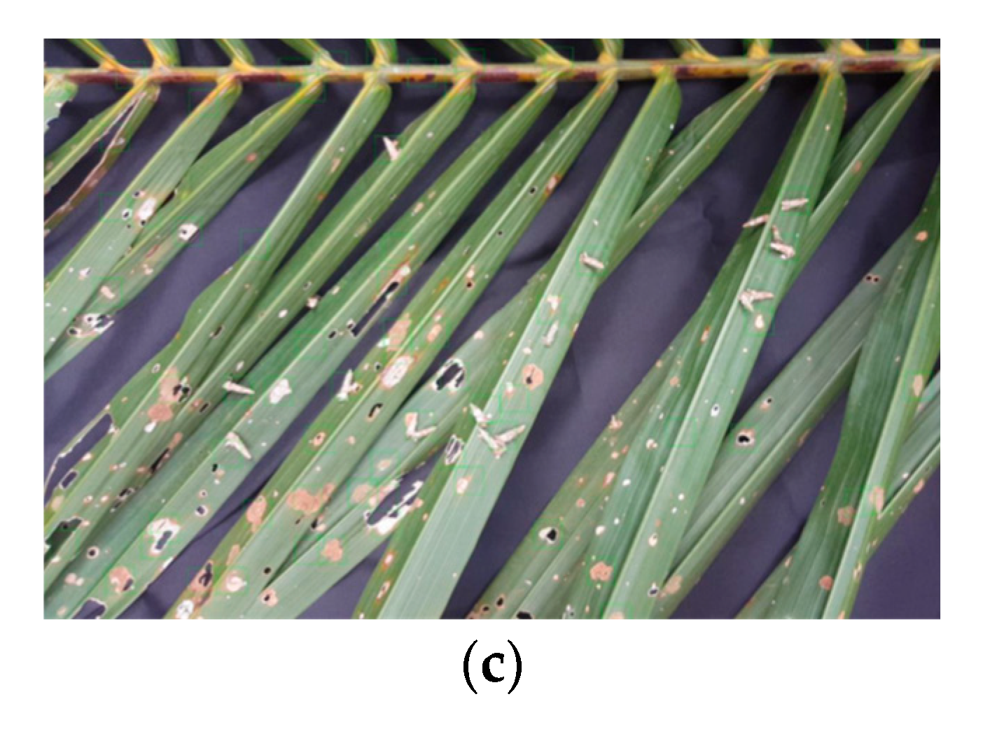
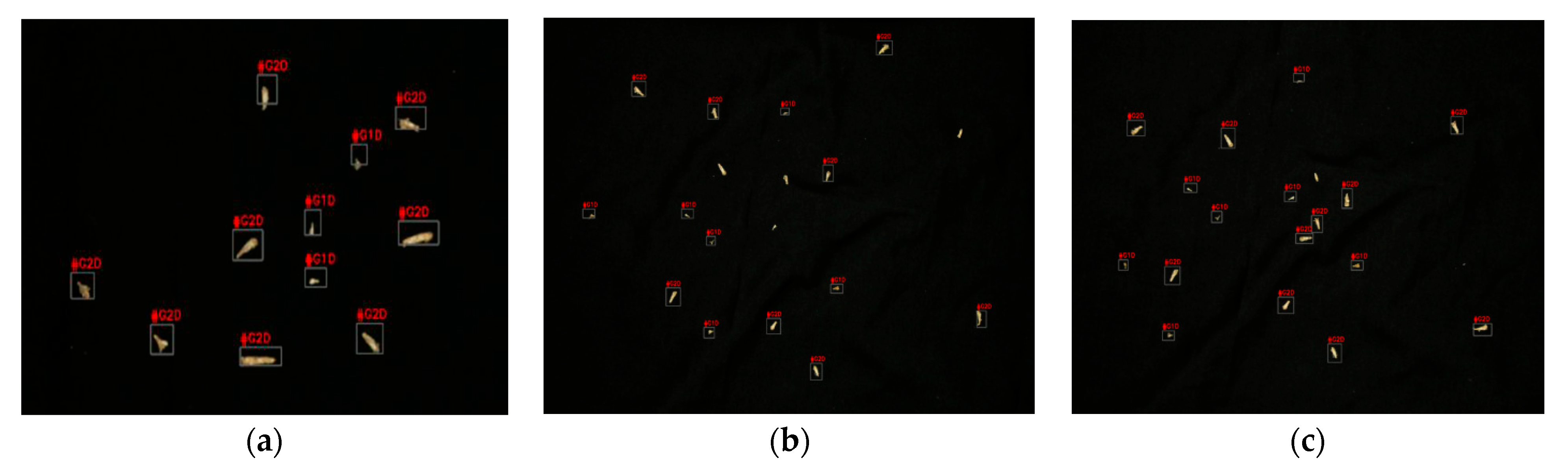
2.3. Third Stage—Object Detection through Deep Learning and Classification
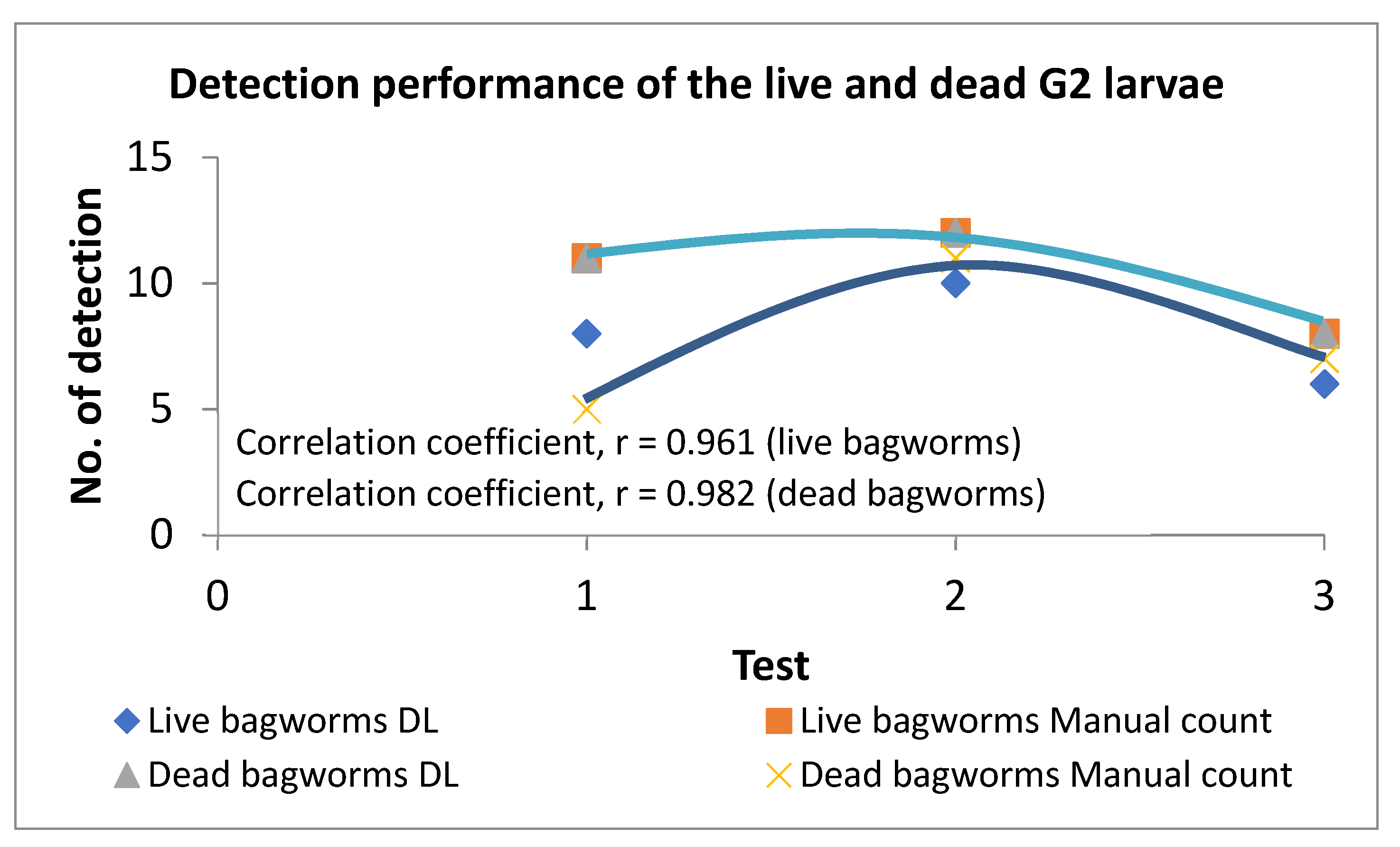
2.4. Fourth Stage—Counting and Determination of the Living and Dead Larvae and Pupae through Motion Tracking and False Color Analysis
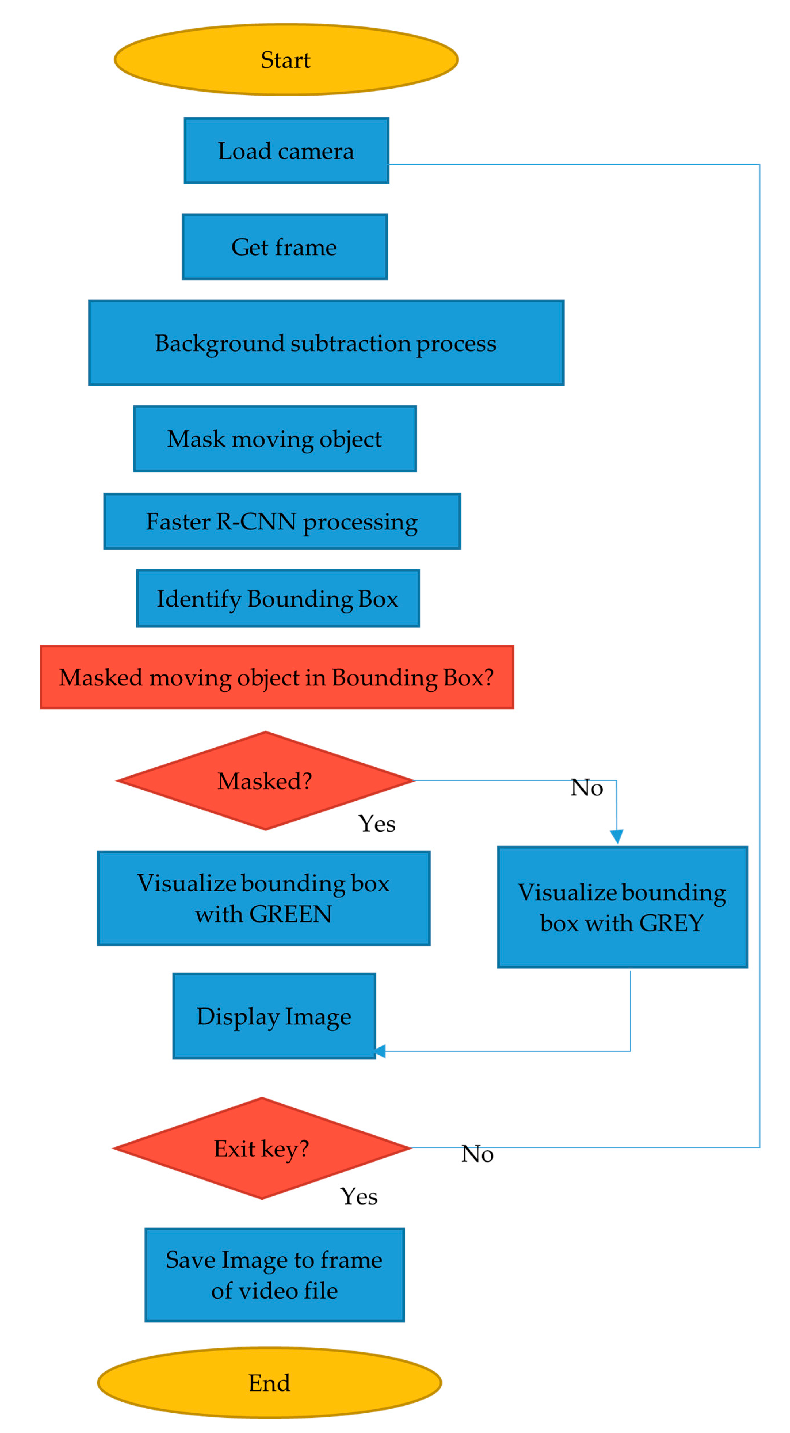
2.5. Motion Tracking for Determination of the Living and Dead Larvae
- Previous frame was processed to be the static background image using BackgroundSubtractorMOG2.
- Current frame was applied to the GaussianBlurr to filter the noise and become the foreground image.
- Masked the background image with the foreground image.
- Applied the cv2.countNonZero of the overlapping background image with the foreground image.
- If there was a nonzero counter, it meant there was movement in the frame.
2.6. False Color for Determination of the Living and Dead Pupae
- Source captured in RGB
- Location of each pupa was marked to calculate the slope value under the red vision (630 nm) as compared to the IR (940 nm) of the pupa at the same location.
- Viewed image in grayscale using OpenCVimshow (img, imgfile, grayscale_option)
- Zoomed each pupa until the pixel value was displayed.
- Picked all the pixels from a pupa image.
- Averaged the pixel values.
2.7. Counting
2.8. Experimental Setup
2.9. Data Analysis
3. Results
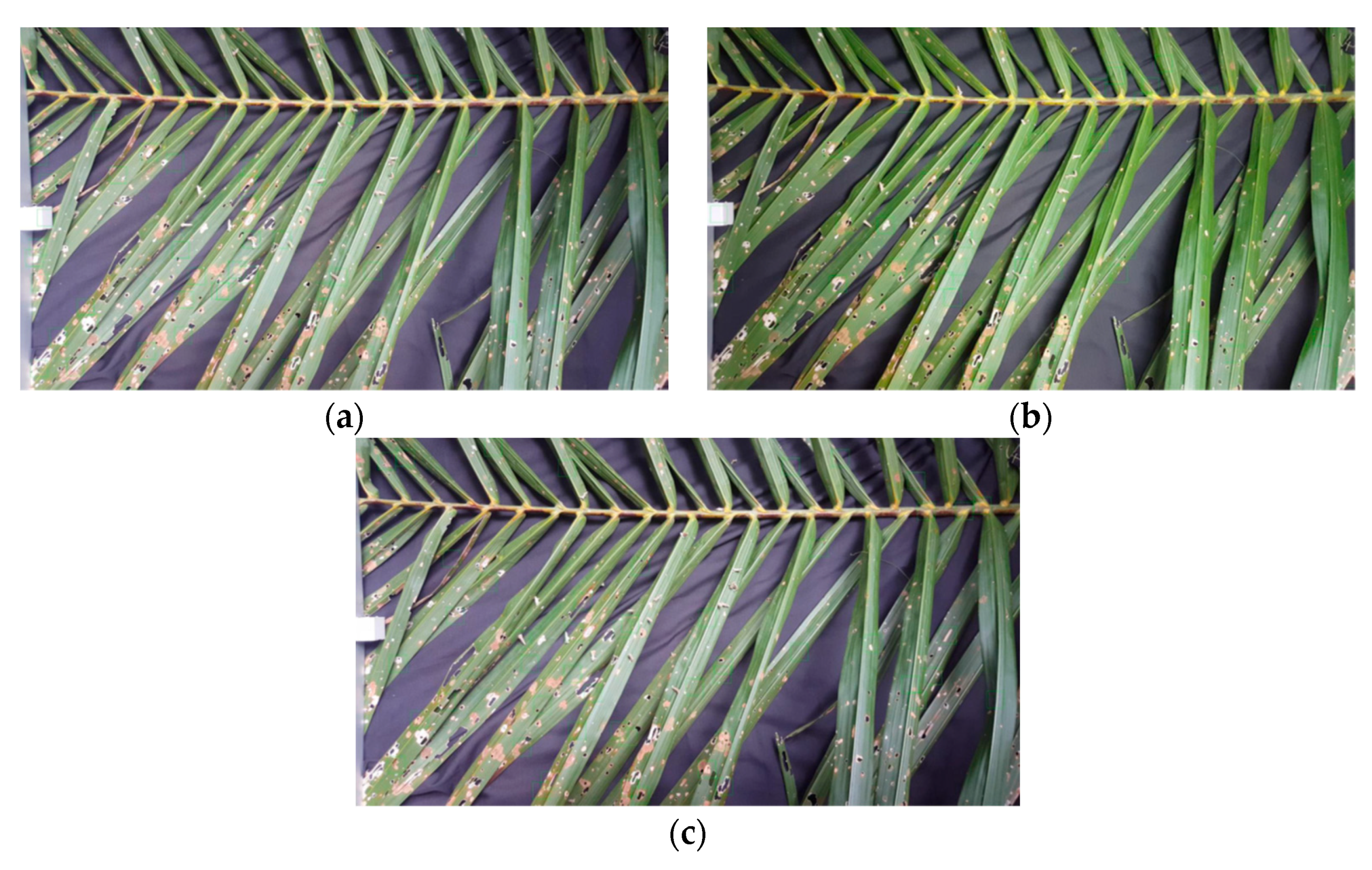
3.1. Stage-1 and 2
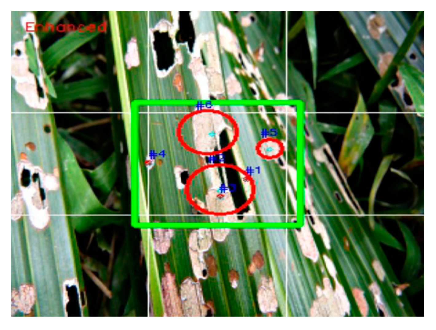
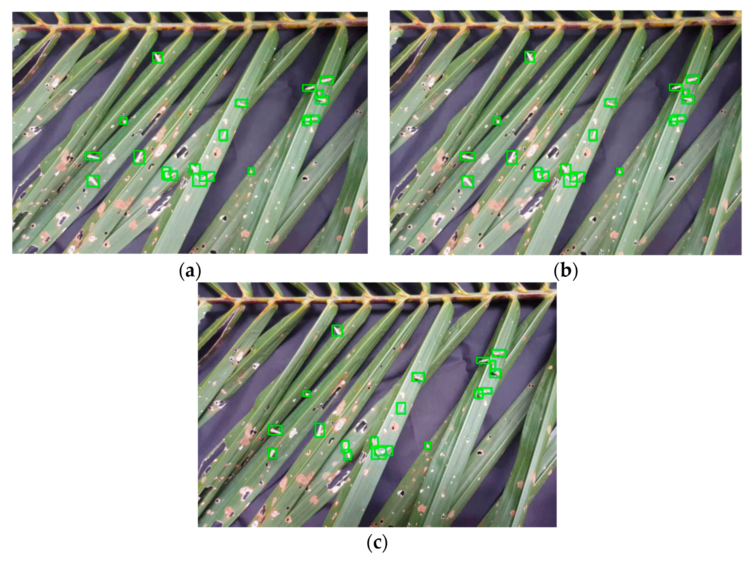
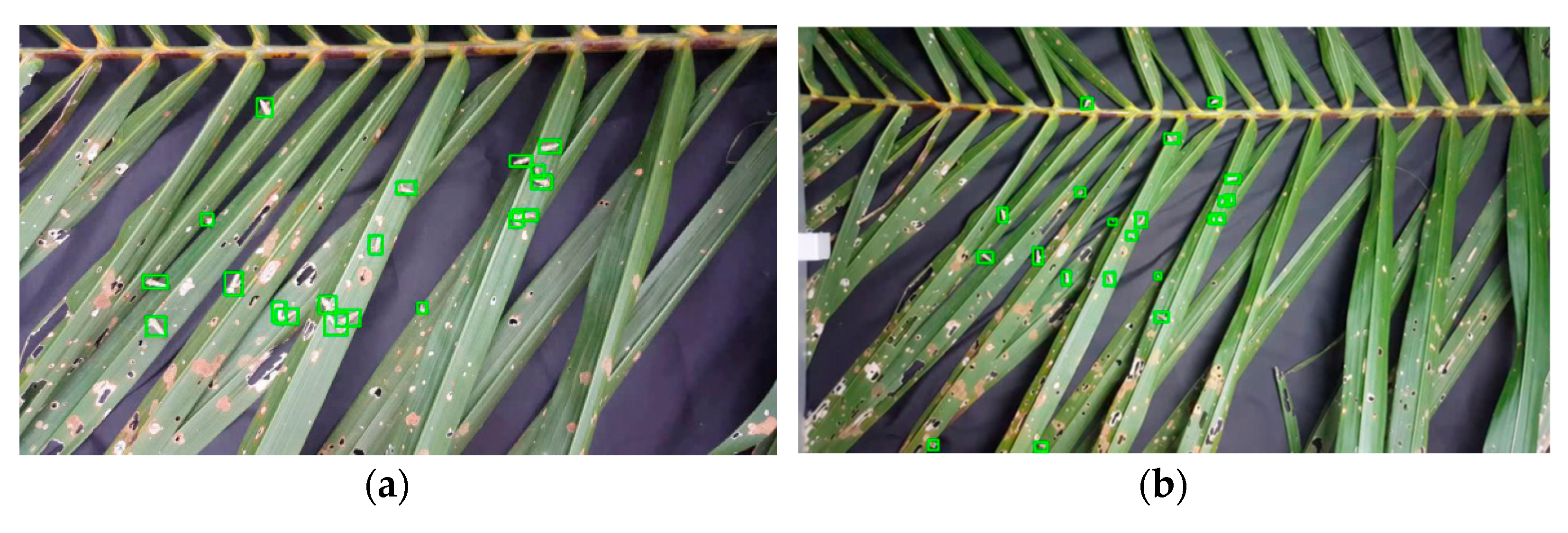
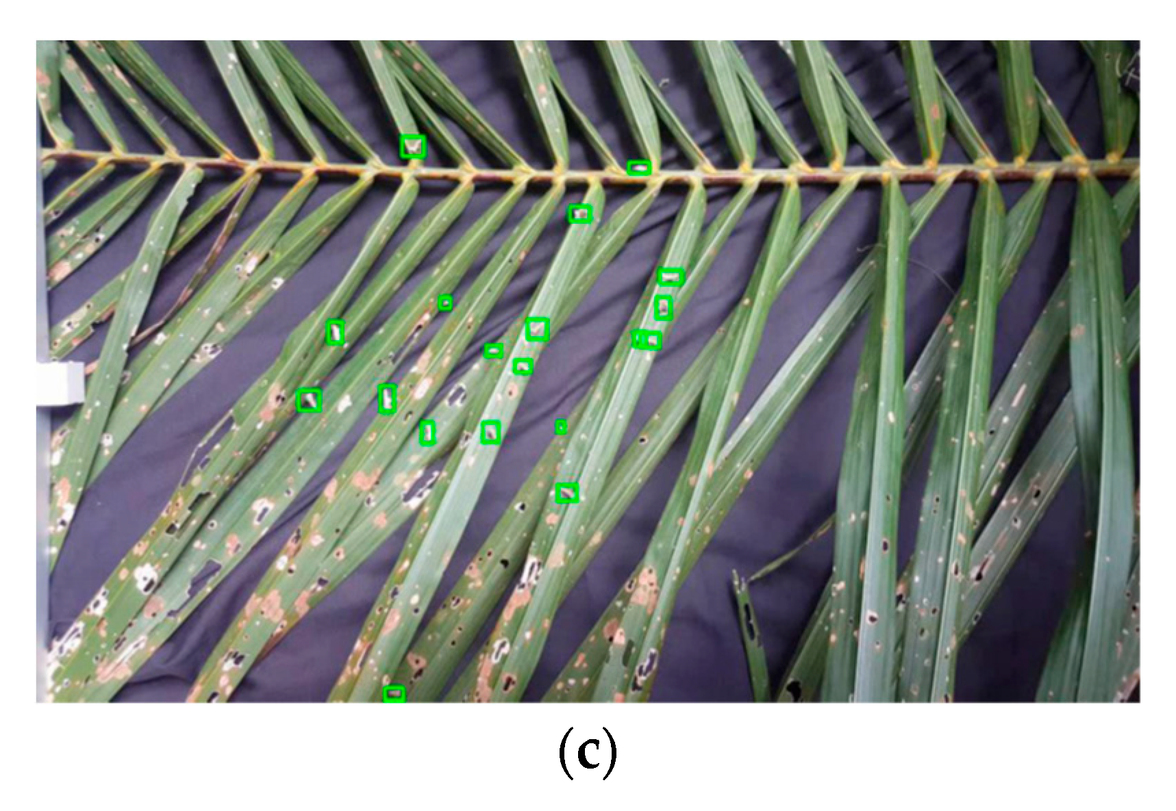
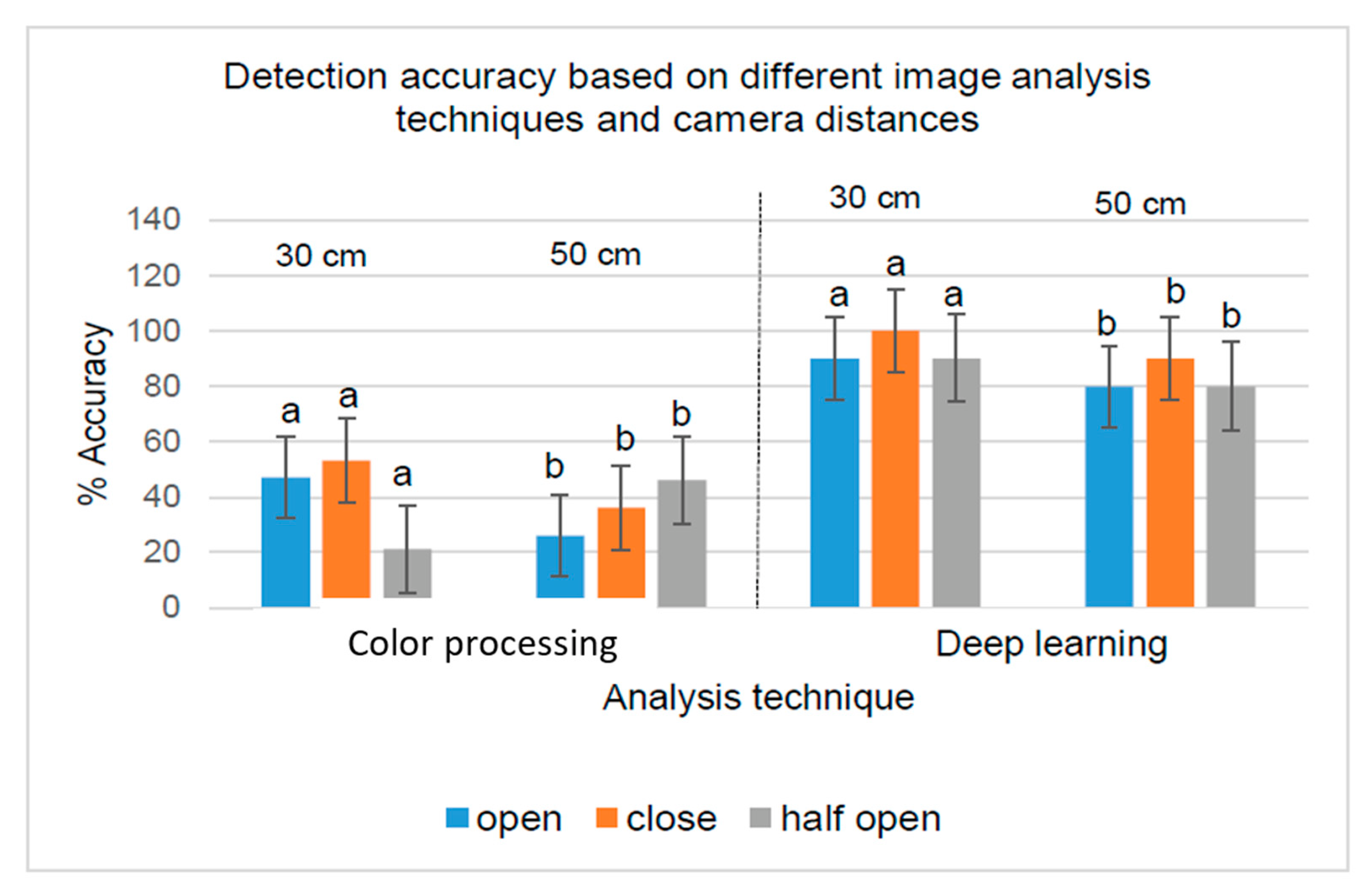
3.2. Stage-3
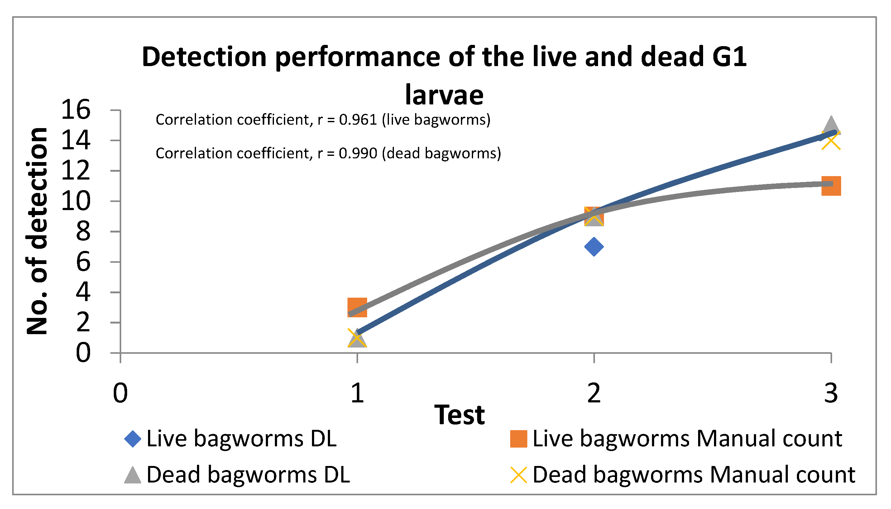
3.3. Stage-4
4. Discussions
5. Conclusions
Author Contributions
Funding
Institutional Review Board Statement
Informed Consent Statement
Data Availability Statement
Acknowledgments
Conflicts of Interest
References
- National Transformation Programme Annual Report. Available online: https://www.pemandu.gov.my/assets/publications/annualreports/NTP_AR2017_ENG.pdf (accessed on 13 May 2018).
- Kushairi, A.; Soh, K.L.; Azman, I.; Elina, H.; Meilina, O.A.; Zanal, B.M.N.I.; Razmah, G.; Shamala, S.; Ahmad Parveez, G.K. Oil palm economic performance in Malaysia and R&D progress in 2017. J. Oil Palm. Res. 2018, 30, 163–195. [Google Scholar]
- Malaysian Palm Oil Board. Standard Operating Procedures (SoP) Guidelines for Bagworm Control; Malaysian Palm Oil Board (MPOB): Bangi, Malaysia, 2016; pp. 1–20. ISBN 978-967-961-218-9. [Google Scholar]
- Ho, C.T.; Yusof, I.; Khoo, K.C. Infestations by the bagworms Metisa plana and Pteroma pendula for the period 1986–2000 in major oil palm estates managed by Golden Hope Plantation Berhad in Peninsular Malaysia. J. Oil Palm Res. 2011, 23, 1040–1050. [Google Scholar]
- Mora, M.; Avila, F.; Carrasco-Benavides, M.; Maldonado, G.; Olguín-Cáceres, J.; Fuentes, S. Automated computation of leaf area index from fruit trees using improved image processing algorithms applied to canopy cover digital photography. Comput. Electron. Agric. 2016, 123, 195–202. [Google Scholar] [CrossRef] [Green Version]
- Shapiro, A.; Korkidi, E.; Demri, A.; Ben-Shahar, O.; Riemer, R.; Edan, Y. Toward elevated agrobotics: Development of a scaled-down prototype for visually guided date palm tree sprayer. J. Field Robot 2009, 26, 572–590. [Google Scholar] [CrossRef] [Green Version]
- Steward, B.L.; Tian, L.F.; Tang, L. Distance-based control system for machine vision-based selective spraying. Trans. ASAE 2002, 45, 1255–1262. [Google Scholar] [CrossRef] [Green Version]
- Amatya, S.; Karkee, M.; Gongal, A.; Zhang, Q.; Whiting, M.D. Detection of cherry tree branches with full foliage in planar architecture for automated sweet-cherry harvesting. Biosys. Eng. 2015, 146, 3–15. [Google Scholar] [CrossRef] [Green Version]
- Balch, T.; Khan, Z.; Veloso, M. Automatically tracking and analyzing the behaviour of live insect colonies. In Proceedings of the 5th International Conference on Autonomous Agents, Montreal, Canada, 28 May–1 June 2001; pp. 521–528. [Google Scholar]
- Uvais, Q.; Chen, C.H. Digital Image Processing: An Algorithmic Approach with MATLAB; CRC Press, Taylor & Francis Group: Boca Raton, NJ, USA, 2010. [Google Scholar]
- Ren, S.; He, K.; Girshick, R.; Sun, J. Faster R C-NN: Towards Real-Time Object Detection with Region Proposal Networks. In Proceedings of the Advances in Neural Information Processing System 25, 24th International Conference, ICONIP 2017, Guangzhou, China, 14–18 November 2017; pp. 91–99. [Google Scholar]
- Yang, Y.; Peng, B.; Wang, J.A. System for Detection and Recognition of Pests in Stored-Grain Based on Video Analysis. In Proceedings of the Conference on Control Technology and Applications, Nanchang, China, 3–5 June 2010; pp. 119–124. [Google Scholar]
- Najib, M.A.; Rashid, A.M.S.; Ishak, A.; Izhal, A.H.; Ramle, M. Identification and determination of the spectral reflectance properties of live and dead bagworms, Metisa plana Walker (Lepidoptera: Psychidae), using Vis/NIR spectroscopy. J. Oil Palm Res. 2020, 33, 425–435. [Google Scholar] [CrossRef]
- Najib, M.A.; Rashid, A.M.S.; Ramle, M. Monitoring insect pest infestation via different spectroscopy techniques. Appl. Spectrosc. Rev. 2018, 53, 836–853. [Google Scholar]
- Najib, M.A.; Rashid, A.M.S.; Ishak, A.; Izhal, A.H.; Ramle, M. A false colour analysis: An image processing approach to distinguish between dead and living pupae of the bagworms, Metisa plana Walker (Lepidoptera: Psychidae). Trans. Sci. Technol. 2019, 6, 210–215. [Google Scholar]
- Badrinarayanan, V.; Kendall, A.; Cipolla, R. Segnet: A deep convolutional encoder-decoder architecture for image segmentation. IEEE Trans. Pattern Anal. Mach. Intell. 2017, 37, 2481–2495. [Google Scholar] [CrossRef] [PubMed]
- He, K.; Zhang, X.; Ren, S.; Sun, J. Deep residual learning for image recognition. In Proceedings of the IEEE Conference on Computer Vision and Pattern Recognition, Las Vegas, NV, USA, 27–30 June 2016; pp. 770–778. [Google Scholar]
- Dai, J.; Li, Y.; He, K.; Sun, J. R-FCN: Object detection via region based fully convolutional networks. Adv. Neural Inf. Process. Syst. 2016, 379–387. [Google Scholar]
- Najib, M.A.; Rashid, A.M.S.; Ishak, A.; Izhal, A.H.; Ramle, M. Development of an automated detection and counting system for the bagworms, Metisa plana Walker (Lepidoptera: Psychidae), census. In Proceedings of the 19th International Oil Palm Conference 2018: Nurturing People and Protecting the Planet, Cartagena, Colombia, 26–28 September 2018. [Google Scholar]
- Simone, W.; Heinz, H.F.B.; Johannes, P.S.; Alexander, T.; Christian, S. Effects of infrared camera angle and distance on measurement and reproducibility of thermographically determined temperatures of the distolateral aspects of the forelimbs in horses. JAVMA Sci. Rep. 2013, 242, 388–395. [Google Scholar]
- Gutierrez, A.; Ansuategi, A.; Susperregi, L.; Tubio, C.; Ivan Rankit, I.; Lenda, L. A Benchmarking of Learning Strategies for Pest Detection and Identification on Tomato Plants for Autonomous Scouting Robots Using Internal Databases. J. Sens. 2019. [Google Scholar] [CrossRef]
- Ding, W.; Taylor, G. Automatic moth detection from trap images for pest management. Comput. Electron. Agric. 2016, 123, 17–28. [Google Scholar] [CrossRef] [Green Version]
- Xie, C.; Zhang, J.; Li, R.; Li, J.; Hong, P.; Xia, J.; Chen, P. Automatic classification for field crop insects via multiple-task sparse representation and multiple-kernel learning. Comput. Electron. Agric. 2015, 119, 123–132. [Google Scholar] [CrossRef]
- Diago, M.; Correa, C.H.; Millan, B.; Barreiro, P.; Valero, C.; Tardaguila, J. Grapevine yield and leaf area estimation using supervised classification methodology on RGB images taken under field conditions. Sensors 2012, 12, 16988–17006. [Google Scholar] [CrossRef] [PubMed] [Green Version]
- Nuske, S.; Wilshusen, K.; Achar, S.; Yoder, L.; Narasimhan, S.; Singh, S. Automated visual yield estimation in vineyards. J. Field Robot. 2014, 31, 837–860. [Google Scholar] [CrossRef]
- Xia, C.; Lee, J.-M.; Li, Y. In situ detection of small-size insect pests sampled on traps using multifractal analysis. Opt. Eng. 2012, 51, 02700. [Google Scholar] [CrossRef]
- Kai, H.; Muyi, S.; Xiaoguang, Z.; Guanhong, Z.; Hao, D.; Zhicai, L. A New Method in Wheel Hub Surface Defect Detection: Object Detection Algorithm Based on Deep Learning. In Proceedings of the International Conference on Advanced Mechatronic System, Xiamen, China, 6–9 December 2017; pp. 335–338. [Google Scholar]


| Group | Bagworm Stages | Real Sizes, mm |
|---|---|---|
| 1 | 1–3 | 1.3–4.4 |
| 2 | 4–7 | 4.5–10.1 |
| 3 | pupal | 10.2–13.6 |
| Camera Distance | Condition | Algorithm Detection | Human Detection | Detection, % |
|---|---|---|---|---|
| 30 cm | Open | 9 | 19 | 47 |
| Closed | 10 | 19 | 53 | |
| Half open | 4 | 19 | 21 | |
| 50 cm | Open | 3 | 19 | 26 |
| Closed | 7 | 19 | 36 | |
| Half open | 9 | 19 | 46 |
| Camera Distance | Condition | Algorithm Detection | Human Detection | Detection, % |
|---|---|---|---|---|
| 30 cm | Open | 9 | 10 | 90 a |
| 30 cm | Closed | 10 | 10 | 100 b |
| 30 cm | Half open | 9 | 10 | 90 a |
| 50 cm | Open | 8 | 10 | 80 a |
| 50 cm | Closed | 9 | 10 | 90 b |
| 50 cm | Half open | 8 | 10 | 80 a |
| Data Samples | Algorithm Detection | Human Detection | Wrong Detection of G1, % | Wrong Detection of G2, % | ||
|---|---|---|---|---|---|---|
| Group 1 | Group 2 | Group 1 | Group 2 | |||
| Figure 15a | 3 | 8 | 3 | 8 | 0 | 0 |
| Figure 15b | 5 | 10 | 6 | 12 | 17 | 17 |
| Figure 15c | 6 | 8 | 6 | 12 | 0 | 33 |
| Groups | Deep Learning Detection | Actual Number of Bagworms | Wrong Detection of Live Bagworms, % | Wrong Detection of Dead Bagworms, % | ||
|---|---|---|---|---|---|---|
| Live | Dead | Live | Dead | |||
| G1 | 3 | 1 | 3 | 1 | 0 | 0 |
| G2 | 8 | 5 | 11 | 5 | 27 | 0 |
| Descriptive Statistics | Spectral Reflectance | False Color Imaging | ||
|---|---|---|---|---|
| Live | Dead | Live | Dead | |
| Mean | 0.26 ± 0.02 | 0.38 ± 0.02 | 0.28 ± 0.02 | 0.34 ± 0.02 |
| Min | 0.26 ± 0.02 | 0.38 ± 0.02 | 0.15 ± 0.01 | 0.30 ± 0.02 |
| Max | 0.27 ± 0.02 | 0.38 ± 0.02 | 0.46 ± 0.01 | 0.46 ± 0.01 |
Publisher’s Note: MDPI stays neutral with regard to jurisdictional claims in published maps and institutional affiliations. |
© 2021 by the authors. Licensee MDPI, Basel, Switzerland. This article is an open access article distributed under the terms and conditions of the Creative Commons Attribution (CC BY) license (https://creativecommons.org/licenses/by/4.0/).
Share and Cite
Ahmad, M.N.; Shariff, A.R.M.; Aris, I.; Abdul Halin, I. A Four Stage Image Processing Algorithm for Detecting and Counting of Bagworm, Metisa plana Walker (Lepidoptera: Psychidae). Agriculture 2021, 11, 1265. https://doi.org/10.3390/agriculture11121265
Ahmad MN, Shariff ARM, Aris I, Abdul Halin I. A Four Stage Image Processing Algorithm for Detecting and Counting of Bagworm, Metisa plana Walker (Lepidoptera: Psychidae). Agriculture. 2021; 11(12):1265. https://doi.org/10.3390/agriculture11121265
Chicago/Turabian StyleAhmad, Mohd Najib, Abdul Rashid Mohamed Shariff, Ishak Aris, and Izhal Abdul Halin. 2021. "A Four Stage Image Processing Algorithm for Detecting and Counting of Bagworm, Metisa plana Walker (Lepidoptera: Psychidae)" Agriculture 11, no. 12: 1265. https://doi.org/10.3390/agriculture11121265
APA StyleAhmad, M. N., Shariff, A. R. M., Aris, I., & Abdul Halin, I. (2021). A Four Stage Image Processing Algorithm for Detecting and Counting of Bagworm, Metisa plana Walker (Lepidoptera: Psychidae). Agriculture, 11(12), 1265. https://doi.org/10.3390/agriculture11121265