1. Introduction
With the introduction of high-throughput plant phenotyping facilities, efficient analysis of large multimodal image data turned into focus of quantitative plant research [
1]. Typical goals of high-throughput plant image analysis include detection, counting or pixel-wise segmentation of targeted plant structures (e.g., whole shoots, fruits, spikes, etc.) in field or greenhouse environments followed by their quantitative characterization in terms of morphological, developmental and/or functional traits. Especially the pixel-wise segmentation represents a critical step of plant image analysis, since the accuracy and reliability of some phenotypic traits (e.g., linear plant dimensions) are highly prone to smallest errors of image segmentation. Due to a number of natural and technical factors, segmentation of plant structures from background image regions represents a challenging task. Inhomogeneous illumination, shadows, occlusions, reflections and dynamic optical appearance of growing plants complicate definition of invariant criteria for detection of different parts (e.g., leaves, flowers, fruits, spikes) of different plant types (e.g., arabidopsis, maize, wheat) at different developmental stages (e.g., juvenile, adult) in different views (e.g., top or multiple side views) acquired in different image modalities (e.g., visible light, fluorescence, near-infrared) [
2]. Next generation approaches to analyzing plant images rely on pre-trained algorithms and, in particular, deep learning models for classification of plant and non-plant image pixels or image regions [
3,
4,
5,
6,
7]. The critical bottle neck of all supervised and, in particular, novel deep learning techniques is availability of sufficiently large amount of accurately annotated ’ground truth’ image data for reliable training of classification-segmentation models. In a number of previous works, exemplary datasets of manually annotated images of different plant species were published [
8,
9]. However, these exemplary ground truth images cannot be generalized for analysis of images of other plant types and views acquired with other phenotyping platforms. A number of tools for manual annotation and labeling of images have been presented in previous works. The predominant majority of these tools including LabelMe [
10], AISO [
11], Ratsnake [
12], LabelImg [
13], ImageTagger [
14], VIA [
15], FreeLabel [
16] are rather tailored to labeling object bounding boxes and rely on conventional methods such as intensity thresholding, region growing and/or propagation, as well as polygon/contour based masking of regions of interest (ROI) that are not suitable for pixel-wise segmentation of geometrically and optically complex plant structures. De Vylder et al. [
17] and Minervini et al. [
18] presented tangible approaches to supervised segmentation of rosette plants. Early attempts at color-based image segmentation using simple thresholding were done by Granier et al. [
19] in the GROWSCREEN tool developed for analysis of rosette plants. A general solution for accurate and efficient segmentation of arbitrary plant species is, however, missing. Meanwhile, a number of commercial AI assisted online platforms for image labeling and segmentation such as for example [
20,
21] is known. However, usage of these novel third-party solutions is not always feasible either because of missing evidence for their suitability/accuracy by application to a given phenotyping task, concerns with data sharing and/or additional costs associated with the usage of commercial platforms.
A particular difficulty of plant image segmentation consists of variable optical appearance of dynamically developing plant structures. Depending on particular plant phenotype, developmental stage and/or environmental conditions plants can exhibit different colors and intensities that can partially overlap with optical characteristics of non-plant (background) structures. Low contrast between plant and non-plant regions especially in low-intensity image regions (e.g., shadows, occlusions) compromise performance of conventional image segmentation tools based on thresholding, region growing or gradient/edge detection. In a number of previous works, transformation of plant images from original RGB to alternative color spaces (e.g., HSV, CIELAB) was reported to be advantageous for separating chlorophyll containing plant from chlorophyll-free non-plant structures in several previous works [
22,
23,
24]. However, in view of high variability of optical setups and plant phenotypes, definition of universal criteria (e.g., color/intensity bounds) for accurate plant image segmentation is not feasible.
To overcome limitations of existing approaches to accurate generation of ground truth data for pixel-wise plant segmentation and phenotyping, here we developed a stand-alone GUI-based tool which enables efficient semi-automated labeling and geometrical editing (i.e., masking, cleaning, etc.) of complex optical scenes using unsupervised clustering of image color spaces. In order to enable a ’nearly real-time’ processing of images of the typical size of several megapixels (i.e.,
n > 1 ×
), unsupervised clustering of image pixels in color spaces was performed using k-means which on one hand is known to be faster than other clustering algorithms such as, for example, spectral or hierarchical clustering [
25]. On the other hand k-means turned out to be efficient and sufficiently accurate for annotation of visible light and fluorescence images of greenhouse cultured plants that were in primary focus of this work. Jansen at al. [
26] used threshold-based approach to segment fluorescence images of arabidopsis plants. We show that using this approach semi-automated labeling of optically complex plant phenotyping scenes can be performed with just a few mouse clicks by assigning pre-segmented color classes/regions to either plant or non-plant categories. By avoiding manual drawing and pixel-wised region labeling, the k-means assisted image segmentation tool (kmSeg) enables biologists to rapidly perform segmentation and phenotyping of a large amount of arbitrary plant images with the minimum user-computer interaction.
3. Experimental Results
The basic idea of our approach to efficient ground truth labeling of plant images consists in automated clustering of image colors followed by selection of plant color classes using the GUI tools. A reliable clustering of images into plant and non-plant classes can, however, be hampered by statistical noise and/or topological vicinity of fore- and background colors in a color space.
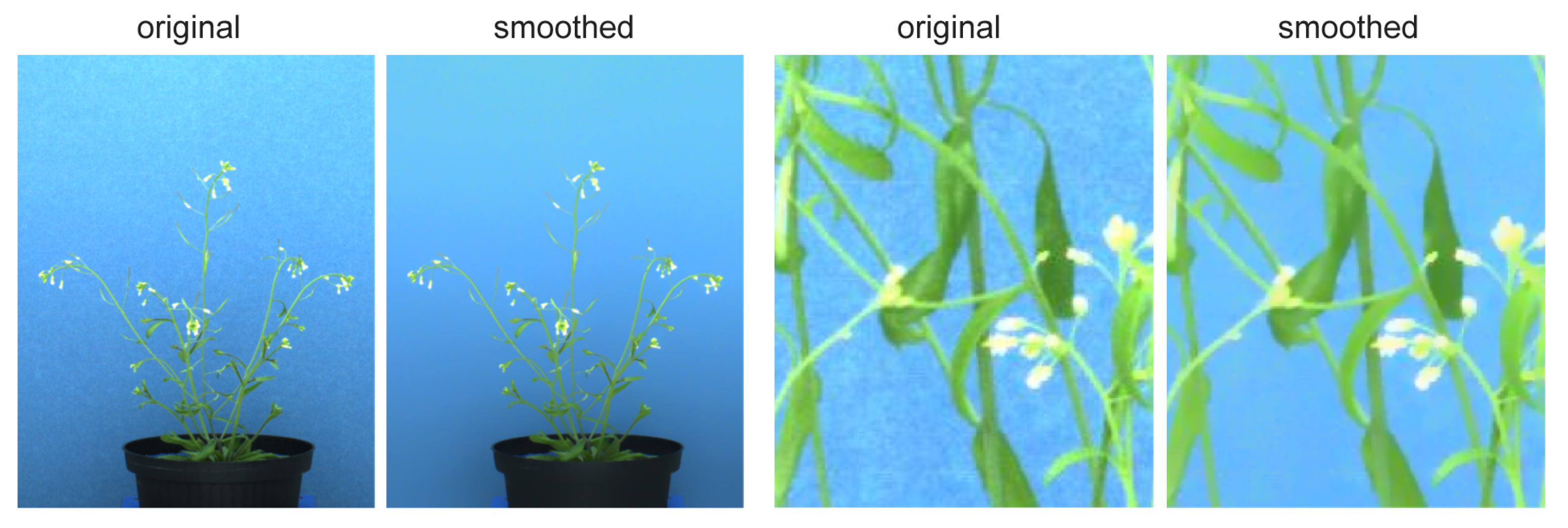
To improve separability of plant and non-plant colors, a structure (edge) preserving Laplace smoothing can optionally be applied in the kmSeg tool.
Figure 4 demonstrates the effect of Laplace smoothing on homogeneity of color distribution in a arabidopsis side-view image. Especially by noisy and low-contrast images, structural enhancement is certainly of advantage for more accurate clustering of basic image color regions.
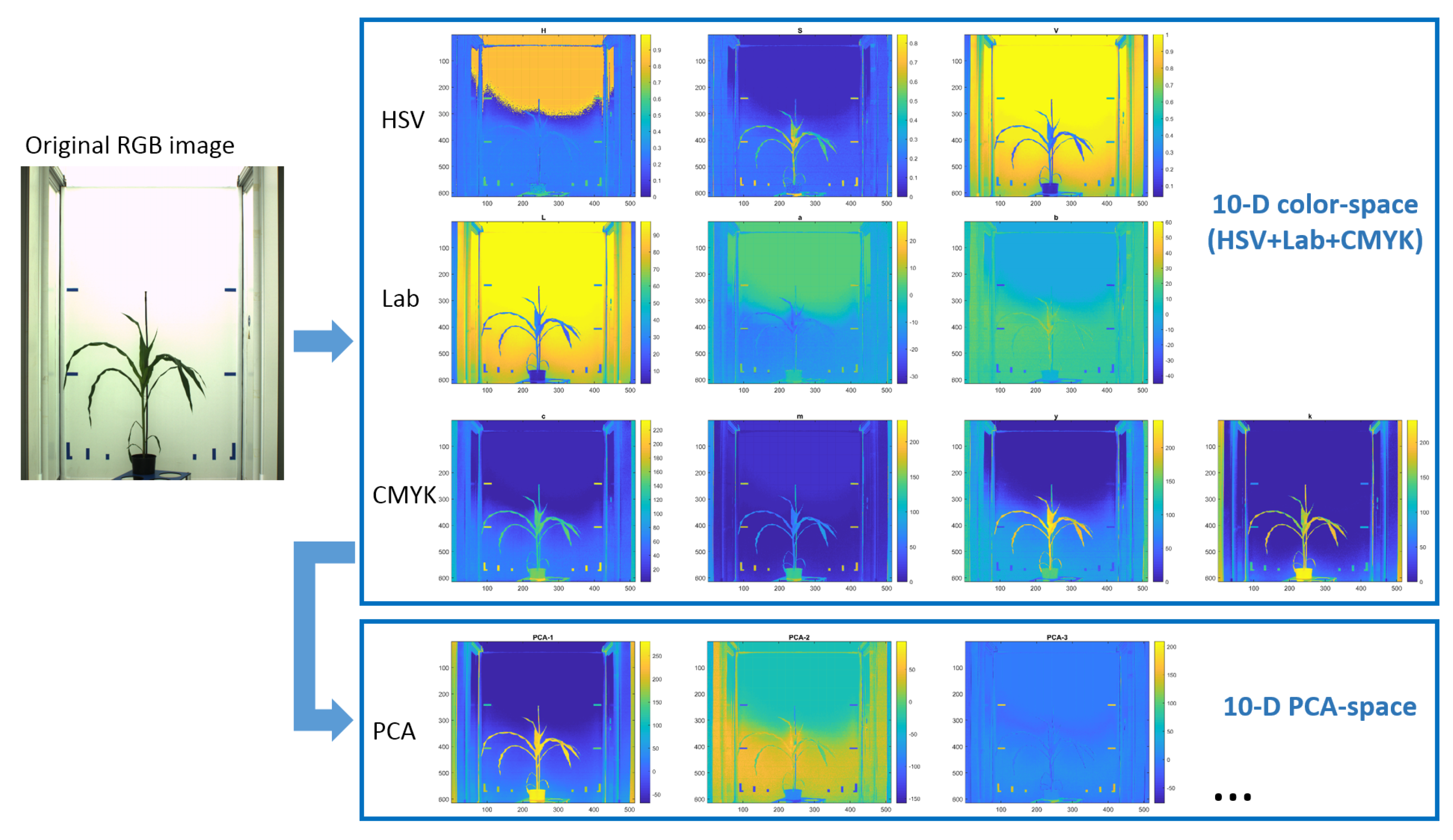
Further important notion is that representation of images in different color spaces can be more or less optimal for separating fore- and background structures.
To quantitatively assess the degree of color decorrelation (
D) in a particular color space, the following criterion was introduced:
where
denotes the percentage of data explained by the
i-the PCA component of the image representation in the
j-th color space. Here, the percentage of data explained by PCA components was calculated using the MATLAB
pca function. The criterion in Equation (
1) was constructed in a way that
takes the value
when image colors are distributed equally over all three PCA components, and the value
when only one single PCA component explains all data.
To systematically assess the degree of color decorrelation in RGB as well as alternative color spaces including HSV, CIELAB, CMYK, the
D criterion in Equation (
1) was calculated for a random selection of 100 greenhouse images. The summary of this performance test of k-means vs. spectral vs. hierarchical clustering algorithms is shown in
Table 1. As you can see the degree of color decorrelation in alternative color spaces (HSV, CIELAB, CMYK) is higher (i.e., the
D value is lower) than in RGB. Otherwise, the
D values of alternative color spaces appears to lay in a relatively close range.
A particularly strong decorrelation effect of the RGB to CMYK transformation can be traced back to the particular MATLAB implementation of the target-oriented transformation to a specific ICC color profile. Conventional RGB to CMYK transformations found in literature cannot have such effect, since they are linear transformations where the key value K is inverse to the V value of the HSV color space. Based on the results of this test, a 10-dimensional image representation in the combined HSV+CIELAB+CMYK color space was used here for subsequent clustering of greenhouse images into fore- and background structures.
For binary classification of image colors into fore- and background regions, different unsupervised methods of data clustering including k-means, spectral or hierarchical clustering can be considered. However, in view of interactive nature of the manual image segmentation an efficient algorithmic performance is required.
To investigate the performance of the above three clustering methods, MATLAB built-in functions
kmeans,
spectralcluster, and
clusterdata were used. In view of a large size of phenotypic images (i.e., >1 ×
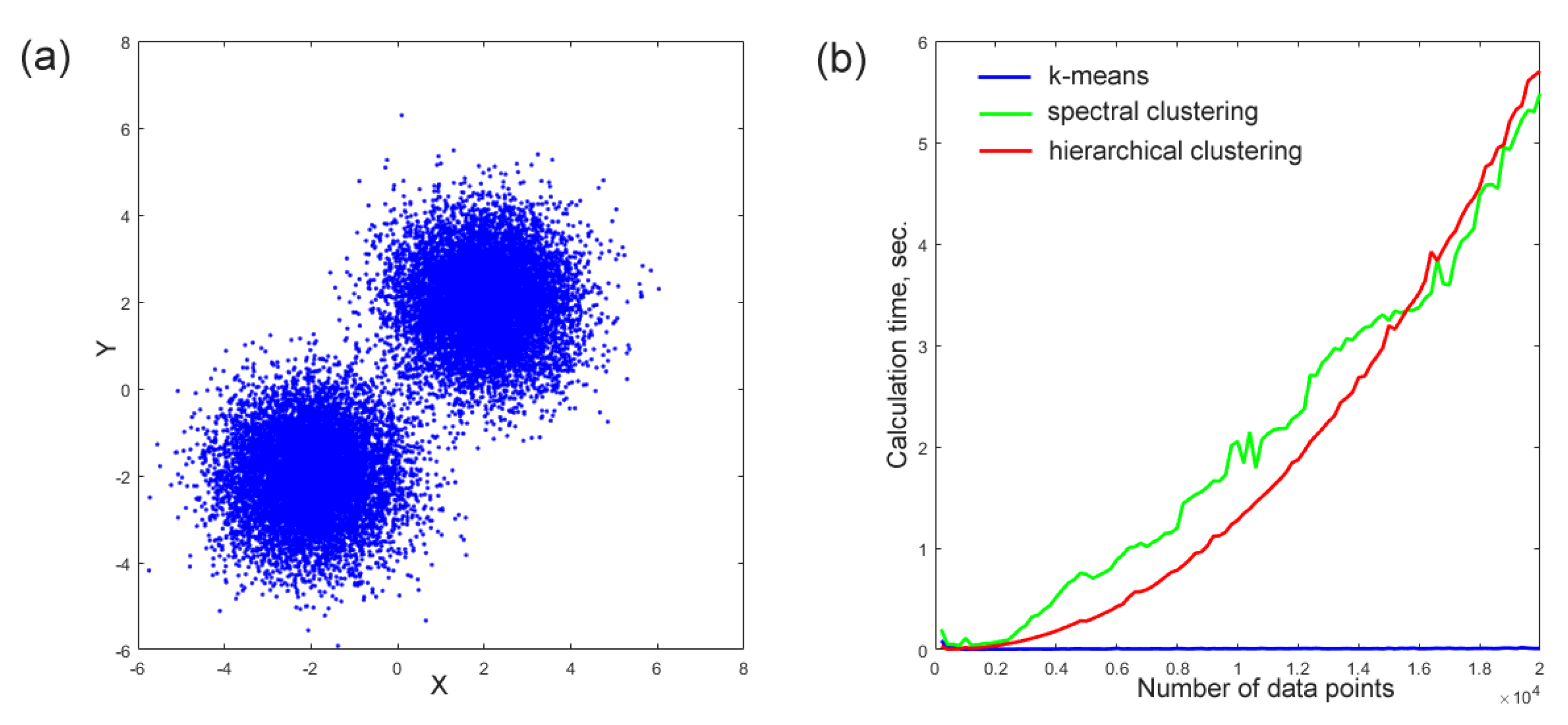
pixels), initial performance tests of clustering methods were performed with synthetic data. For this purpose, a series of parametrically identical two-dimensional bi-Gaussian distributions of different size in the range between 400 and 40,000 points were generated.
Figure 5a shows an example of such a bi-Gaussian distributed point cloud used in this test. The three above clustering algorithms were applied to a series of these synthetic point distributions with the goal to separate them into two clusters corresponding to the two original bi-Gaussian distributions, and to assess their performance in term of calculation time. The results of these performance tests shown in
Figure 5b demonstrate that spectral and hierarchical clustering algorithms are computationally too expensive and, thus, cannot be applied for processing images of typical megapixel size within a reasonable period of time. In contrast, the k-means clustering algorithm has shown an acceptable performance. The MATLAB code of this performance test can be found in
Algorithm S1.
Consequently, fast k-means clustering was adopted in this work for pre-segmentation of fore- and background image colors in the 10-dimensional Eigen-color space.
The basic approach to plant image segmentation in this work consists in unsupervised k-means clustering of image Eigen-colors followed by manual selection of color classes corresponding to the targeted plant structures, e.g., shoots, leaves, flowers, fruits. To optimize the result of unsupervised k-means clustering, a number of additional image pre-processing steps such as image filtering an/or ROI masking can be applied.
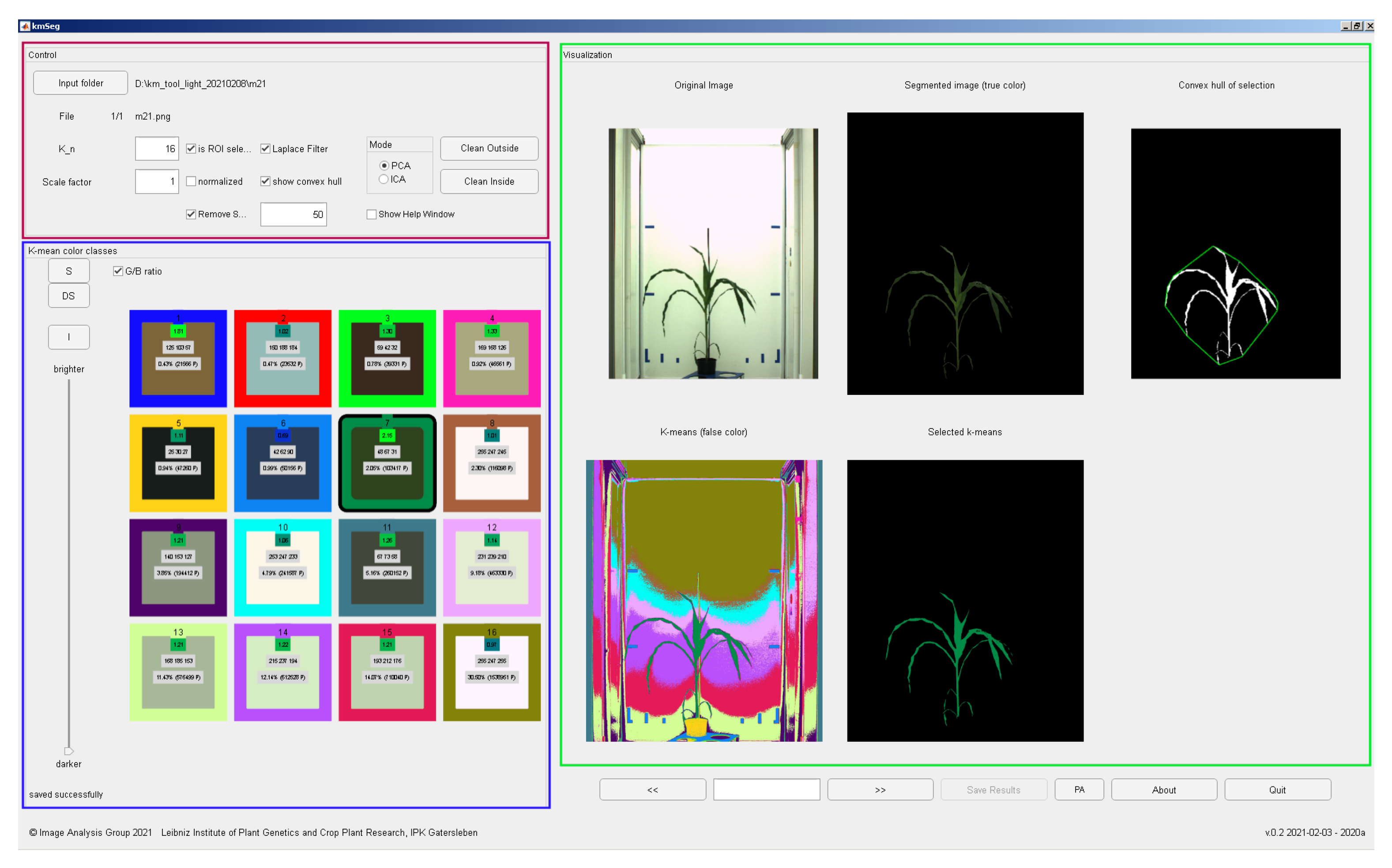
To enable users efficient processing and analysis of image data, the above described algorithmic framework was implemented as a GUI tool.
Figure 6 shows a screenshot of the kmSeg tool including three major GUI elements: ’Control’, ’k-means color classes’ and ’Visualization’ areas.
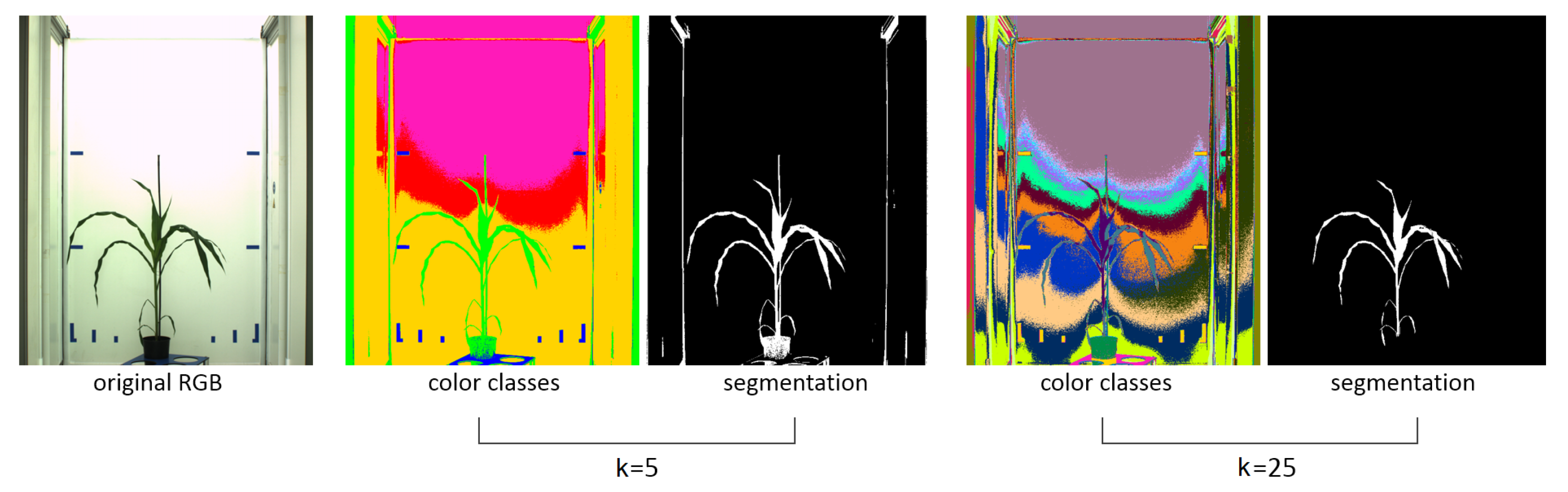
The work with the kmSeg GUI begins with selection of a target file directory in the ’Control’ area containing one or more images stored in *.png or *.jpg formats. Once an image directory is selected and images are successfully imported into the program, the calculation immediately starts using the default set of algorithmic parameters including the number of k-means classes, the image scaling factor and filters that can afterwards be adjusted by the user. As rule of thumb, the higher the number of k-means classes is chosen the more fine and potentially more accurate separation of plant and non-plant structures can be achieved.
Figure 7 shows an example of segmentation of a maize image using k = 5 and k = 25 k-means color classes, respectively.
A typical number of k-means classes for segmentation of greenhouse plant images ranges between 9 and 36 depending on complexity of color image composition. Fully automated determination of the number of k-means classes is not necessarily advantageous in this application, since users may want to adjust the algorithmic performance for optimal color separation and image segmentation based on their visual inspection. Depending on complexity of image colors, users can explore and select an optimal number of k-means classes by trying and evaluating the results of image segmentation for a number of guesses, e.g., k = 9, 16, 25, 36. Furthermore, in the ’Control’ area, user can define the type of color space transformation (PCA or ICA), optional downscaling ratio for faster processing of large images, image smoothing and filtering as well as visualization of the resulting convex hull of segmented ROI can be activated here. Changes in the ’Control’ area automatically trigger re-calculation of image segmentation with the actualized set of parameters.
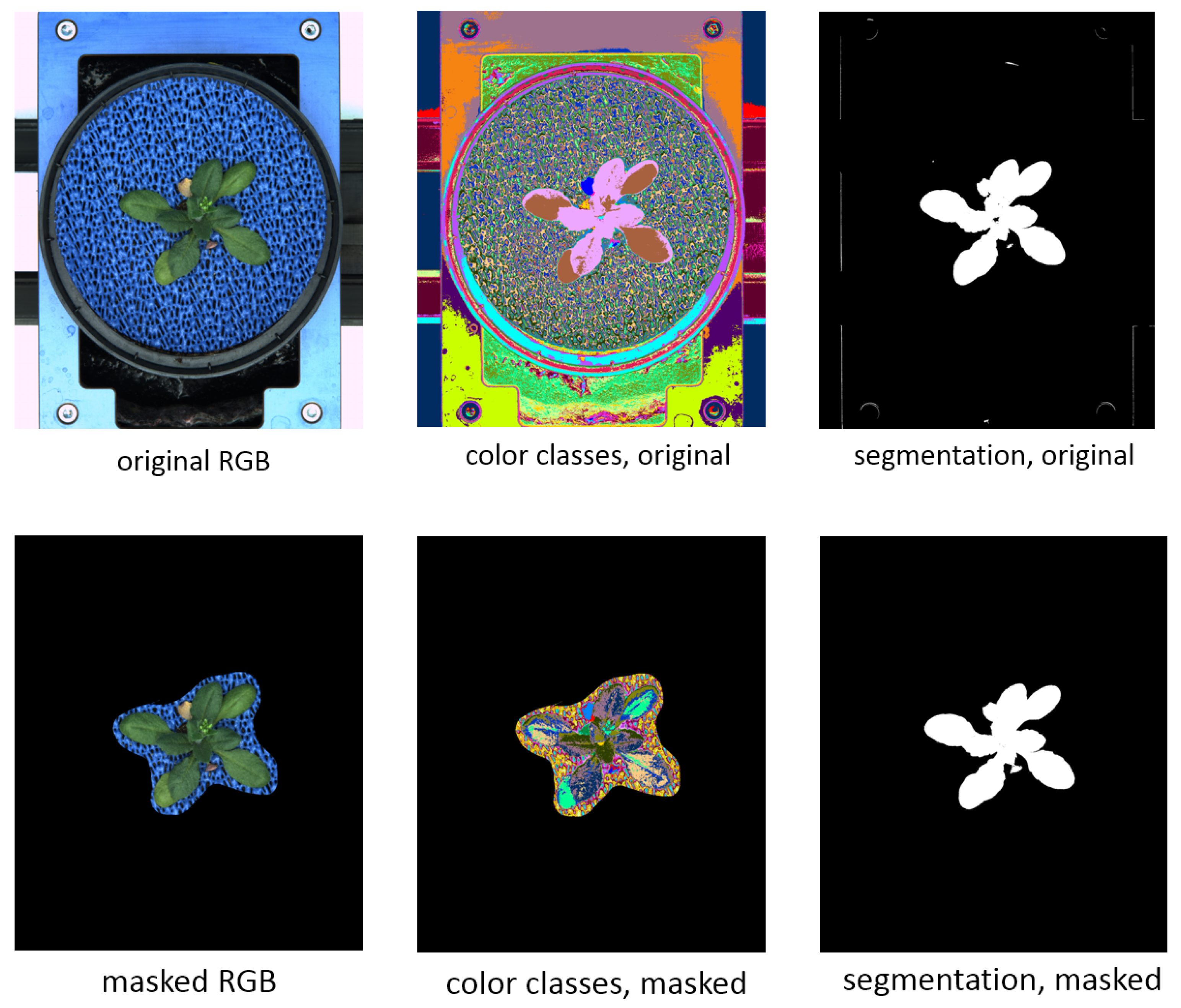
To restrict automatic pre-segmentation to a particular region of interest two functions ’Clean Inside’ and ’Clean Outside’ are provided in the ’Control’ area. They allow the user to clean up the regions outside or inside of a freehand-drawn polygon around a particular ROI (e.g., plant). ROI masking allows the user to avoid artifacts due to faulty segmentation of shadows or reflection in the background region that are, for example, frequently observed on the boundaries of photo chambers. Furthermore, masking of the plant ROI reduces the complexity of color distributions which effectively shortens the calculation time and improves the accuracy of fore- and background color separation for the same number of k-means classes.
Figure 8 shows an example of top-view arabidopsis image, where such masking was required to achieve a good segmentation result.
The movie
https://ag-ba.ipk-gatersleben.de/kmseg_movie.html, (accessed on 11 February 2021) demonstrates all steps of the kmSeg application to segmentation of the arabidopsis image from
Figure 8 which took approximately 2 min on a Intel i7-6700HQ powered consumer-notebook with 16 GB RAM. Further examples of ROI masking for efficient segmentation of visible light and fluorescence arabidopsis, barley and maize shoot images in side- and top-views are shown in
Supplementary Information (Figures S1–S12). Although, the kmSeg tool was primarily developed for processing of images of greenhouse-grown plants, it can also be applied to other image data that can principally be segmented by means of color clustering. Further examples of the kmSeg application including segmentation of fruits, flowers, leaf speckles, and multi-stain microscopic images can be found in
Supplementary Information (Figures S13–S18).
The ’k-means color classes’ area enables visual inspection and manual assignment of pre-calculated k-means color classes to either plant or non-plant categories. Here, the user is supported by a number of numerical indicators including
running number of the k-means color class,
the mean RGB values of the color class,
the green-to-blue (G/B) ratio of the color class which is typically larger than one for plant structures,
percentage of the total area of the color class,
absolute number of pixels (area) of the color class.
Furthermore, spatial regions corresponding to all and selected color classes can be inspected in in sub-figures of the ’Visualization’ area depicting pseudo-color, original RGB, binary segmentation with an optional convex hull visualization, see
Figure 6. Assignment of pre-segmented color classes to plant or non-plant categories is performed by a single click on the icon of the k-means color class which corresponds to the targeted ROI. Renewed clicking on the selected color icon deselects the k-means class and assigns it to another category (e.g., from plant to non-plant category). After the first manual assignment of plant/background categories to colors of k-means regions, plant/background categorization of color regions in subsequent images is automatically extrapolated from the last manual segmentation. It can be, however, changed by the user anytime. By using the ’go back’ or ’go forward’ buttons, the previous or the next image can be selected. Instead of clicking several times, the user can directly jump to the sought image by entering its running number in the list of all images in the selected folder. By pressing the ’Save results’ button the user saves all segmentation results in a subfolder of the source image directory.
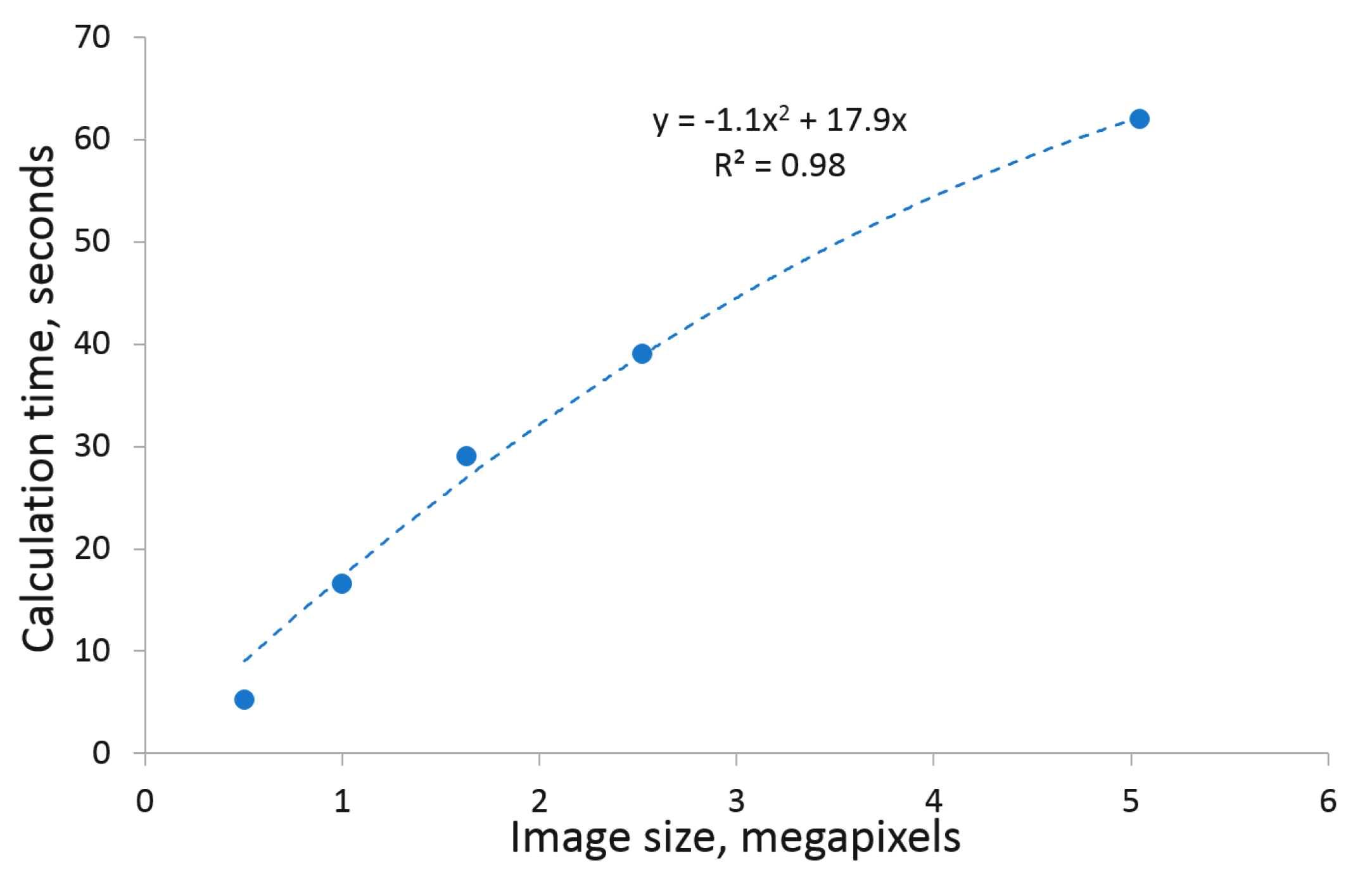
In general, segmentation of images using the kmSeg tool depends on the size of images and/or selected ROIs.
Figure 9 shows a summary of k-means clustering (i.e., the first automated step toward image segmentation) of up to 5 megapixel large images, which lays in the range between 5–60 s. In comparison, fully manual image segmentation using conventional tools (e.g., thresholding, manual drawing and cleaning in ImageJ) is expected to be several times more time consuming, depending on the user’s skills, software choice and image complexity.
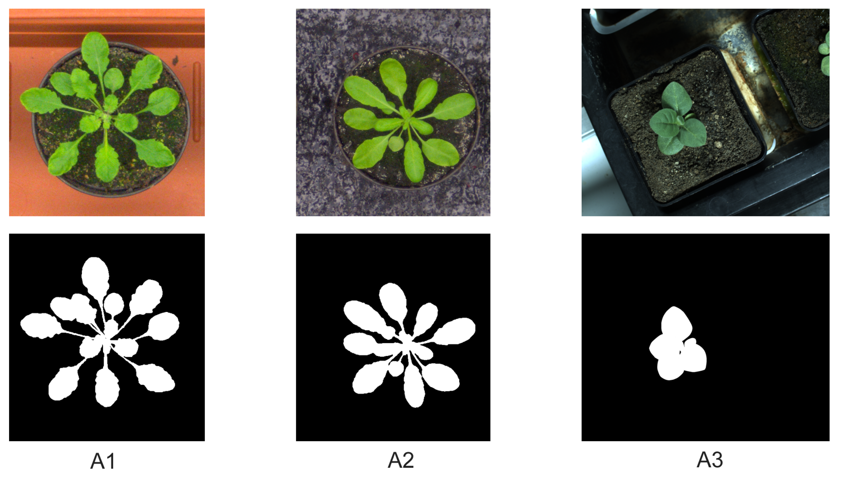
To quantitatively assess the accuracy and performance of the kmSeg tool by segmentation of different plant images, original and complementary ground truth images from A1, A2, A3 datasets published in [
8] were used. All images were processed as described above using 36 k-means classes for clustering of PCA-transformed 10 dimensional (HSV+CIELAB+CMYK) image representation, followed by optional ROI masking, selection of plant color classes and image cleaning.
Table 2 gives a summary of the kmSeg performance indicating that typical top-view plant images can be segmented and analyzed using the kmSeg tool within 2–6 min with an average accuracy (i.e., the Dice similarity coefficient) ranging between 0.96–0.99. Thereby, the most time consuming and less accurate segmentation results were observed for A1 images that exhibit a larger variation of colors and background vegetation with a similar color fingerprint as arabidopsis leaves. A2 and A3 images with higher plant-background contrast were segmented more efficiently and accurately.
As output of image segmentation, the kmSeg tool writes out following files
segmented images including labeled color classes, RGB and binary images, see the ’Visualization’ area in
Figure 6,
a *.csv file containing basic traits of segmented plant structures including descriptors of plant area, shape and color fingerprints in RGB, HSV, CIELAB color spaces, see the full list in
Supplementary Information (Table S1),
a plain ASCII file describing assignment of k-means classes to pseudo-colors of plant and non-plant regions,
Figure S19a,
a copy of the entire MATLAB workspace (
*.mat file) of the kmSeg tool containing segmentation results and help-variables,
Figure S19b.
*.mat files containing the entire internal kmSeg tool variables, that can be used by MATLAB users for a detailed analysis or serve for debugging purposes. Segmented images and complementary ASCII files allow users to retrieve all information necessary for quantitative description of segmented plant and non-plant image regions.
The precompiled executable of the kmSeg tool along with the user guide and examples of greenhouse plant images is provided for download from
https://ag-ba.ipk-gatersleben.de/kmseg.html, accessed on 11 February 2021.


