Methodology for Measurement of Ammonia Emissions from Intensive Pig Farming

Abstract

Determination of ammonia (NH₃) emissions for intensive livestock facilities (pork, poultry) is important from both a regulatory and a research point of view. Buildings housing livestock are a large source of ammonia emissions from the agriculture sector. However, measurements to determine emissions can be time-consuming and costly. Therefore, it is essential to find a suitable methodology for monitoring NH₃. The methodology for determining NH₃ emissions is legislatively unified in terms of sampling methodology, including sampling time (24 h), sampling points (input/output), number of sampling days, and their distribution during the year, and to determine only a general calculation of the annual average NH₃ emissions. For this reason, the researchers chose different approaches for the calculation of NH₃ emissions, and these approaches are not unified. Based on accurate monitoring and created models, the authors proposed a methodology for calculation of NH₃ emissions, which divides the 24 h measurement into time windows (30 min), from which the arithmetic mean and standard deviation are determined, and the total emissions for one year is determined. The chosen time windows for the partial calculation are important from the point of view of reflecting the microclimatic conditions inside the stable and the device limits for sampling the NH₃ concentration and airflow.

1. Introduction

At present, NH₃ is a significant air pollutant, and its concentration does not decrease rapidly. The reduction in ammonia emissions has been slow over the last three decades, particularly compared to the reduction in emissions of other pollutants such as nitrogen oxides (NO_x), sulfur dioxide (SO₂), and non-methane volatile organic compounds [1]. In principle, NH₃, as a pollutant gas, accelerates the formation of fine particles in the atmosphere. Ammonia is crucial for the acidification and eutrophication of ecosystems and consequently contributes to climate change [2,3].

In addition to the environmental aspects, particulate NH₃ also has a negative impact on human health [4]. Due to the biogenic and anthropogenic origin of atmospheric ammonia, it is particularly harmful to human health, especially to the eyes and respiratory systems [5,6,7]. Exposure to ammonia is accompanied by clinical symptoms such as coughing, sneezing, salivation, excessive lachrymal secretions, loss of appetite, and lethargic behavior [8,9]. Ammonia also participates in reactions forming organic and inorganic aerosols that can adsorb a high concentration of toxic air pollutants, which affects human health by mutagenic and genotoxic activities [10,11,12].

The agro-industry is considered the primary contributor of NH₃ in most developed countries [1,13,14]. Due to demographic growth and changes in food preferences, global NH₃ emissions are expected to double by 2050 [2,15]. The major source of NH₃ in agriculture is livestock excreta emitting NH₃ immediately after deposition and during decomposition. Reactions of urease enzyme or microbial activity quickly release NH₃ to the atmosphere, consuming unconverted nitrogen originating from high-protein feeds used to fulfill nutritional requirements [16]. From the chemical point of view, nitrogen-based emissions are probably caused by ammonia (NH₃-N) losses from the interconversion of total ammoniacal nitrogen (NH₃-N + NH₄⁺-N) and organic nitrogen, eventually by the aqueous equilibrium of (NH₃-N) and (NH₄⁺-N) [17].

Ammonia has a perceptible odor even at very low concentrations, and its emissions are mainly observed in locations with high-density livestock farming, especially in pig farms [18]. Pig farming is globally responsible for about 15% of NH₃ emissions associated with livestock breeding [19]. The main source of NH₃ releases from buildings with daily housing emission factors of 34.3–146.4 g NH₃ per 500 kg live weight for fattening pigs [20]. The amount of nitrogen-based emissions also depends on the type of housing and technologies, waste management, environmental conditions (e.g., temperature, wind speed, enzymatic activity, pH, relative humidity), and efficiency of utilizing nitrogen by the animal [21,22].

The precise identification and determination of NH₃ emissions seems essential both for meeting legislative standards (identifying the effectiveness of mitigation strategies at the national and regional level, preparing national annual emission inventories for regulatory purposes) and developing technologies aimed at reducing these emissions [23].

As NH₃ emissions are complex and depend on many factors, the effort is made to determine the resulting emissions from farms as accurately as possible. Three approaches have been identified for this purpose. Two of them estimate the total emissions over each manure management phase (housing, manure storage, landspreading), and the third approach determines only emissions from housing.

The first one estimates the value on the basis of a mass balance based on the excretion and total nitrogen, or total ammoniacal nitrogen (TAN), present at each manure management phase. Ammonia emissions are estimated based on the amount of nitrogen excreted by each animal category and using the total nitrogen or TAN flow and the volatilization coefficients over each manure management phase (housing, manure storage, landspreading).

The second one is an estimation by application of emission factors. Ammonia emissions are estimated on the basis of emission factors derived from measurements designed and performed according to a national protocol in a farm with an identical type of technique (housing, manure storage, landspreading) and similar climatic conditions.

For this above approach, methodologies (models) have been developed and approved, which calculate these emissions on the basis of data from operating conditions. These methodologies are used in European Union countries, and they are time-saving but less accurate.

The third possibility estimates emissions by a calculation from measured values of ammonia concentration and ventilation rate only from housing. This method is more accurate in comparison with the two above-mentioned methods. Their outputs are based on methodologies for estimation of emissions by calculation, and they are used to determine the emissions produced accurately, to verify the use of Best Available Technologies (BAT), but it is more time- and money-consuming. In addition, it is methodically complete in terms of measurement methodology (data collection in the stable), but the algorithm for evaluating the emissions from the measured data is not explicitly defined [24,25].

The Directive 2010/75/EU of the European Parliament and of the Council, for the intensive rearing of poultry or pigs, defines the general principles of the estimation of ammonia emissions. Pig farming is characterized as a category of animals with a linear increase in emissions per breeding cycle; therefore, the days on which NH₃ emissions are measured must be evenly distributed over the period of their growth. Ammonia emissions must be evaluated in at least six sampling days over a period of a breeding cycle. This means that three measurements are evenly distributed in the first half of the breeding cycle and three further measurements in the second half of the breeding cycle. The annual ammonia emissions are calculated from the mean of the one-day emissions obtained during six 24 h measurements multiplied by the number of days of stable occupancy by animal [26].

Sampling is carried on at the air inlet and outlet of the stable for 24 h. Ventilation performance is also measured (alternatively it can be generated from the ventilation control unit). The concentration of NH₃ in the air output from the stable is measured, adjusted to the concentration of the inlet air to the stable, and the daily NH₃ emissions are derived by measuring and multiplying the ventilation and NH₃ concentration. The annual average NH₃ emissions are determined from the daily average NH₃ emissions multiplied by the number of days of stable occupancy by animal [26].

Despite many devices, the measurement of NH₃ emissions has not usually been implemented in day-to-day monitoring due to the high specialization of each device, making it difficult to use them in typical farming situations. At any rate, the measurement of NH₃ in pig farms and development of an appropriate measurement methodology are necessary to increase agricultural efficiency and, consequently, the quality of life and the environment. Generally, NH₃ measurement methodology includes selecting a suitable monitoring system, sampling configuration of the used device, the additional equipment for measuring other physical quantities, the spatial and layout arrangement of used equipment in the pig house, and the method of statistical analysis of obtained data.

There is obviously a strong need for unification in order to compare the research data with each other effectively. Thus, the aim of this study is to provide an accurate and effective methodology for measuring and statistically evaluating NH₃ emissions in pig houses based on performed experiments and previous studies.

2. Materials and Methods

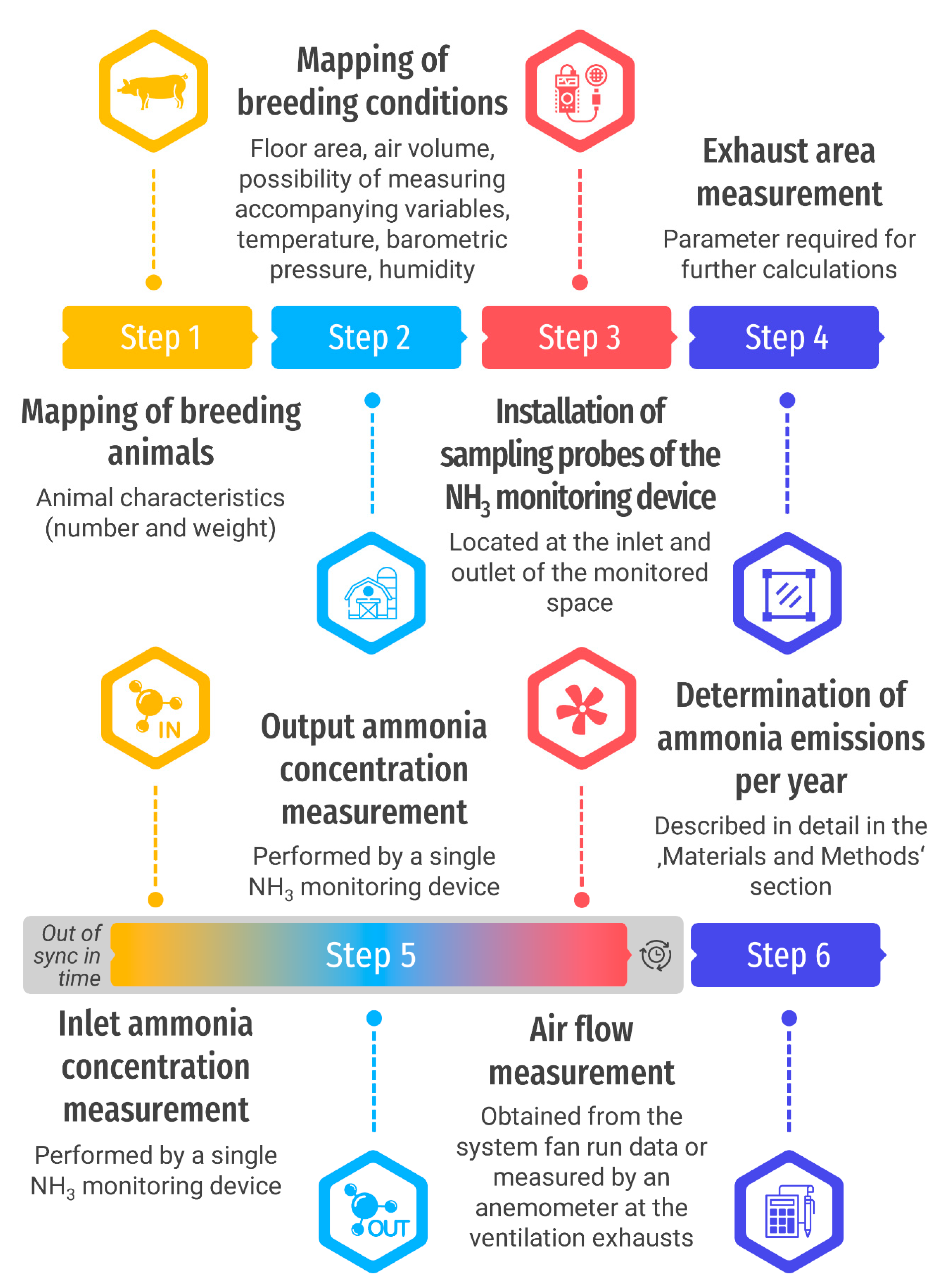
2.1. Scheme of Methodology

The overview schema of methodology for measurements and determination of the ammonia emissions from intensive livestock farming is below in the Figure 1. This methodology is described in detail in the following chapters.

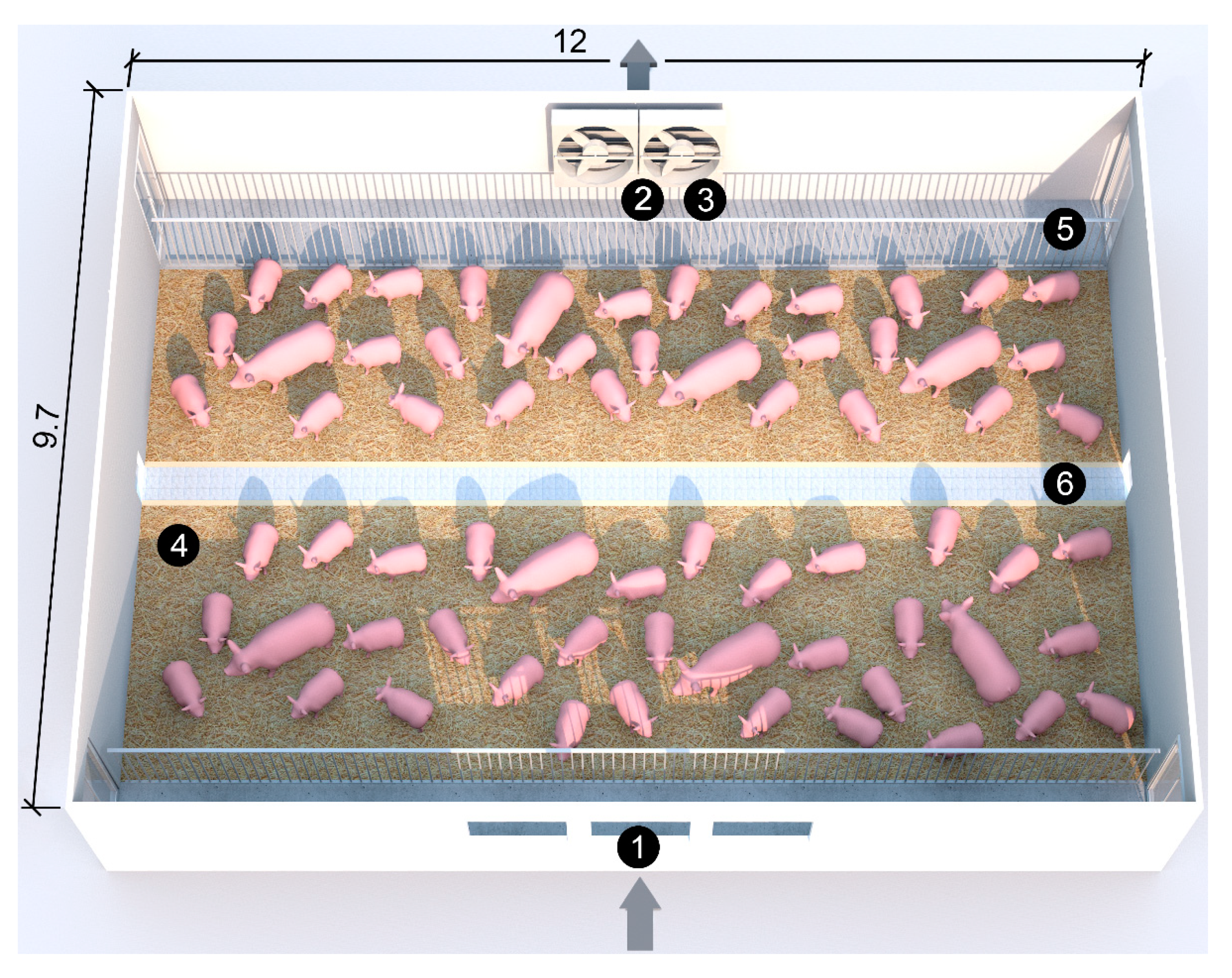
2.2. Experimental Pig House

The study was carried out in a pig production house located in the Czech Republic in the district of Tabor at an altitude of 455 m (GPS coordinates 49°15′03″ N, 14°33′01″ E). The stable for breeding sows with piglets (mating and gestating sows) was divided into five pens, each with a concrete floor with deep straw litter (BAT 30.a6) and middle corridor for assessing the manure. There were service alleyways on both sides. An automatic feeding system for moist feed for phase feeding (BAT 3.b) was situated in every pen. In every breeding section, negative pressure ventilation was addressed by two wall ventilators by diametral 0.45 m, which automatically control the indoor microclimate. Outdoor air was sucked in by three 0.8 × 0.3 m wall openings. The data collecting was performed in one selected pen, which is illustrated in Figure 2. At the time of monitoring, there were 12 sows and 76 piglets in the pen.

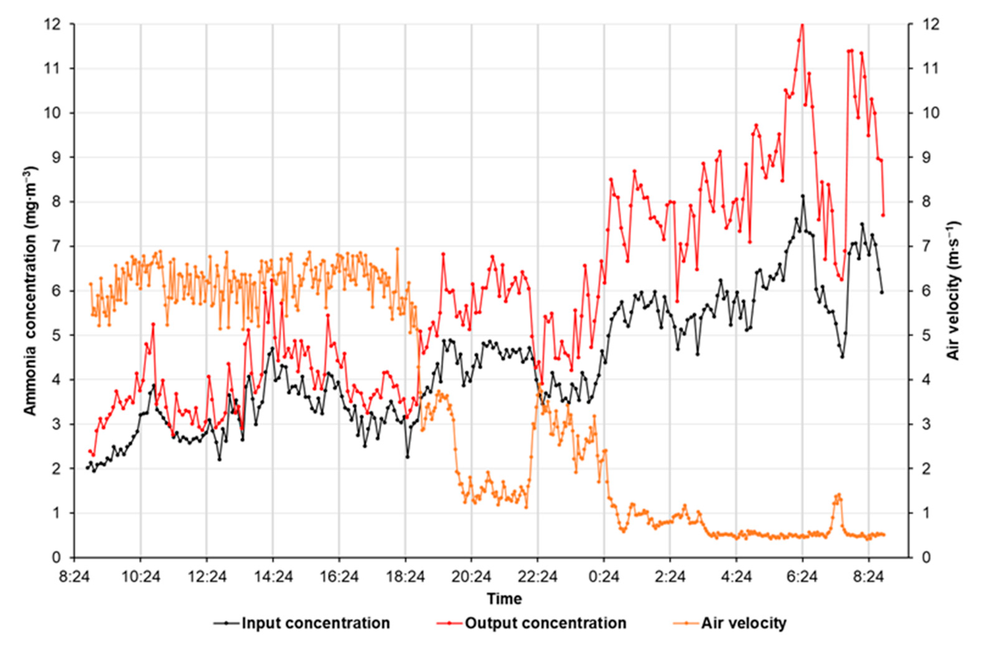
2.3. Methodology for Measurements of the Ammonia Concentration in the Pig Farm

Ammonia concentration measurements were performed simultaneously at the air inlet and outlet from the stable continuously for 24 h. A photoacoustic multigas monitor INNOVA 1412 by LumaSense Technologies A/S, Ballerup, Denmark, equipped with a multi-channel sampling and dosing device Multipoint Samplet 1309 D or similar devices are recommended to be used for the NH₃ concentration measurement. From the measuring device, special Teflon hoses were stretched to the sampling points (air inlet and outlet). The device continuously uploading the measured values to its internal memory, while the sampling frequency was set to once every 6 min. At the same time, other physical quantities (indoor and outdoor temperature, relative humidity, atmospheric pressure) were monitored during the measurement using a multi-purpose device (COMMETER D4141, COMET SYSTEM spol. s r.o., Rožnov pod Radhoštěm, Czech Republic), and the airflow rate in the exhaust fans was measured by means of an anemometer (TESTO 445, TESTO AG, Lenzkirch, Germany).

2.4. Methodology for Calculation of NH₃ Emissions

The determination of NH₃ emissions in the stable is based on the data from measuring ammonia concentrations in the air entering and exiting the stable. Another parameter for finding out the emission is the determination of the airflow outwards. Last but not least, it is necessary to know the area of the vents exhaust and also the number of housed animals for the purposes of determining the total production of specific NH₃ emissions per year. The measurement of the input and output NH₃ concentration is usually performed by INNOVA 1412 with two sensors connected; therefore, it is not possible to obtain data from both sensors at the same time. In addition, the airflow through the stable ventilation is usually determined independently of the concentration measurement time. It is either obtained from the stable system data on the operation of the fans or is directly measured by an anemometer at the ventilation exhausts. In both cases, there is no group of three corresponding data points available to calculate the NH₃ emission rate. For this reason, it is necessary to calculate emissions from several independently measured data points of all input variables during a suitably selected time interval, the so-called time window. Its length must be chosen carefully with regard to the accuracy of measurement but also to the problem of monitoring NH₃ production in the stable during the day.

The ammonia emission rate E (mg∙s⁻¹) can be now figured out from this formula:

E = (C_OUT − C_IN)∙v∙S,

(1)

where C_OUT is NH₃ concentration in an outlet (mg∙m⁻³), C_IN is NH₃ concentration in the input (mg∙m⁻³), v is air velocity by venting the stable (m∙s⁻¹), and S is the area of the exhaust of the stable vents (m²).

The arithmetic mean and standard deviation are determined from all obtained values of effective emissions during one day (24 h). Subsequently, the total production-specific emissions per year E_YEAR (kg∙animal⁻¹∙year⁻¹) are determined and converted to a value per pig using this formula:

E_YEAR = E_AVG∙N⁻¹,

(2)

where E_AVG is arithmetic mean of the E (kg∙year⁻¹), and N is the number of pigs housed in the stable.

2.5. Creation of Model Data for Method Testing

For the purpose of creating a methodology for evaluating NH₃ emissions from stables, model data of monitored variables were firstly created. Because the input values for the calculation (input and output NH₃ concentration and gas flow through the stable vents) are not interdependent quantities, the input data for the model were based on real measured data. From these data, a simple regulation simulating the stable situation was created (see Figure 3).

Breakpoints were identified based on the visual evaluation of the course of individual quantities; their values were roughly determined with an accuracy of 0.5 mg∙m⁻³ or 0.5 m³∙s⁻¹, respectively, including their time offset from the starting time (integral multiples of 0.5 h). The entire waveforms of the input quantities were then replaced by a polyline connecting the above-mentioned points. Furthermore, the normally distributed noise was added to the concentration values, with a mean value of 0 and a standard deviation of 0.5 for the input concentration and 0.9 for the output concentration, respectively. From the measured data it was evident the input concentration fluctuated less than the output concentration; therefore, a different standard deviation was chosen in the model. In the case of flow values, the fluctuation depends on the absolute value of the measured flow; at higher flow rates, it fluctuates more; at lower flow rates, the fluctuation is significantly lower. Therefore, the flow values on the polyline were multiplied by a coefficient having a Gaussian distribution with a mean value of 1 and a standard deviation of 0.05. The resulting model is shown in Figure 4.

For the purpose of testing the evaluation methodology, the second set of model data was created based on the original model and where, in addition, the data were artificially modified at randomly selected time intervals. In the time interval from 3:14:17 to 4:14:17, the model data were sorted so the input concentration C_IN decreased continuously throughout this hour, while the output concentration C_OUT and the airflow v continuously increased. This situation simulates the maximum possible error load in the E evaluation due to the impossibility of measuring all input variables simultaneously. This will lead to the largest fluctuations in the calculation of the E. In the time interval from 11:55:13 to 12:55:13, both the input concentration C_IN and the output concentration C_OUT were arranged in ascending order, and the air flow fluctuated in the usual manner. This adjustment best corresponds to the real situation due to the interdependence of both concentrations of ammonia, i.e., that the trend of both concentrations was the same (in this case, growth). The last adjustment was made in the time interval from 18:44:40 to 20:44:40, when the air flow was set equal to zero. This simulates the failure of the anemometer or system flow sensors in the stable. The modified model data are in the graph in Figure 5; the vertical green lines indicate the intervals in which the model data were artificially modified.

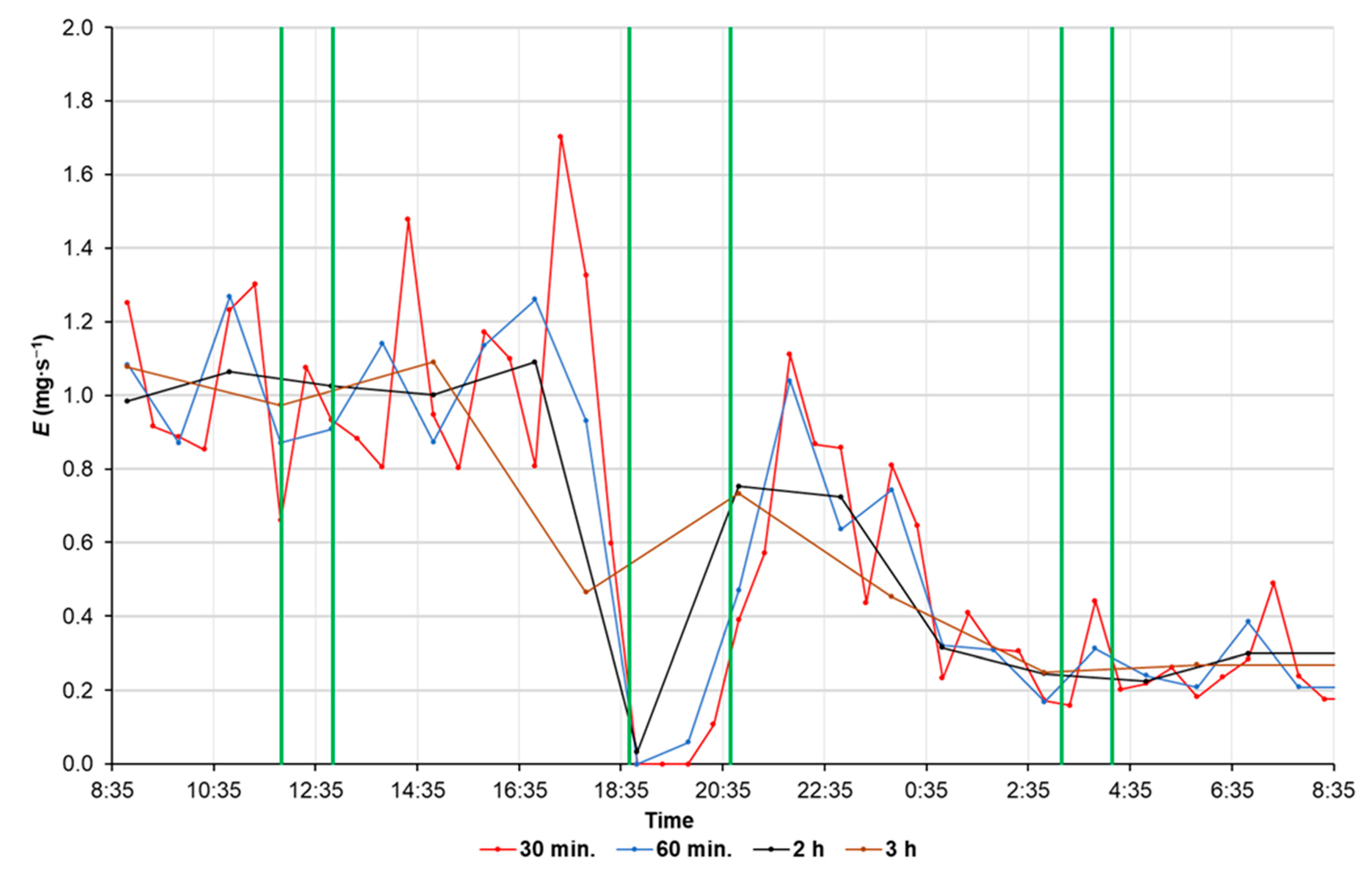
2.6. Testing the E Evaluation Method

The reference E_ref value was determined for testing of the developed methodology of the evaluation of ammonia emissions. It was determined analytically from Equation (1) on the basis of the known equations of the individual parts of the polylines from which the input variable waveforms were created (see Section 2.5).

We divided the methodology tests into two parts. The proposed E evaluation methodology was applied in every case. In the first part, we investigated the effect of the time window length on the average ammonia emissions over 24 h. The time window length was gradually chosen from a series of 15 min, 20 min, 30 min, 45 min, 60 min, 90 min, 2 h, 3 h, 4 h, 6 h, 8 h, and 12 h. The area of the vents exhaust and the number of housed animals corresponded to the real situation on which the model was based (see Section 2.2).

At first, the methodology was tested on a model polyline with no added noise to determine the effect of time window length on the total ammonia emissions. The obtained values were compared with the analytical E_ref reference using relative percentage deviation. Subsequently, the methodology was applied to both the unmodified model with added Gaussian noise and the artificially modified model to calculate ammonia emissions. The differences between the individual calculated values were tested using ANOVA analysis and Tukey’s HSD test. Differences between calculated emissions of given time window lengths for both models were tested also by Student’s t-test. The significance level of every statistical test was 0.05.

In the second part of the methodology testing, only a few windows were selected, and the influence of their length on the course of the specific emission curves during 24 h was monitored. As no statistically significant differences were found in the first phase of testing, no statistical method was not used in this part, but the calculated diurnal wave-forms were visually compared to each other.

3. Results

The reference ammonia emission E_ref was analytically determined to be 0.5767 mg∙s⁻¹ and 1.5157 kg∙animal⁻¹∙year⁻¹. The relative deviations of the calculated emissions of the model data without added noise were increased with increasing time window length. The lowest value of 0.17% was reached for the shortest 20 min time window. Similarly, for longer time windows up to 60 min it did not exceed 1.00%. On the contrary, the highest value was calculated for the time window of 24 h length, where it reached up to 52.60%. However, despite the rather significant relative deviation, even ANOVA analysis together with Tukey’s HSD test showed no statistically significant difference (p > 0.999), which may be due to the small sample size in the case of longer time windows.

The same E evaluation algorithm with time window selection was used for both unmodified and modified model data. The obtained E values for individual windows are shown in Figure 6 (unmodified model) and in Figure 7 (modified model). Both graphs show that with the increasing length of the time window, the average value of E increased, initially very slowly. For longer time windows the increase was more pronounced (for the time window of 12 h, E was more than 10% higher than for the time window of 15 min). The standard deviation also increased because 24 h of data was processed, which decreased the total number of time windows with its increasing length. Figure 6 shows that for time windows up to 2 h, the increase in E was very small, almost imperceptible (increase was less than 2.5% compared to the value for the 15 min time window), which implies that the effect of time windows of 2 h and below was practically negligible for the calculation of the average E.

A similar situation can be observed in the case of an artificially modified model in Figure 7. Modifications to the model generally reduced the size of the average E, which corresponds to a zero contribution to the average E in the period simulating the failure of the anemometer. However, the modifications did not affect the trend of its dependence on the time window length. The increase in E for time windows up to 2 h did not exceed 3%, but at 12 h the time window was almost 15% higher than the calculations for the 15 min time window. Artificially created short-term singularities in the time courses of measured quantities thus had a very small effect on the average values of E when using the developed evaluation methodology with time windows up to 2 h. We can assume that the mentioned singularities will not be present at all in real data, or they will be of shorter duration than was modeled, and thus will not affect the resulting specific annual NH₃ emissions.

In the second part of the methodology testing, only four-time windows were selected (30 min, 60 min, 2 h, and 3 h), and the influence of their length on the course of the specific emission curves during 24 h was monitored. The respective waveforms are shown in Figure 8 (unmodified model) and Figure 9 (modified model). It is clear from the waveforms for the individual time windows that the increasing length of the window significantly reduced the fluctuations of the calculated value of ammonia emissions; on the other hand, it significantly eliminated the actual fluctuations of the emissions during the day. For the time window of 3 h, it is possible to determine only the all-day trend of NH₃ emissions in the stable, and it is not possible to identify shorter-term singularities based on it.

When comparing the course of the polylines in Figure 8 and Figure 9, the influence of artificial modifications of model data on the actual course of the curves was well visible. While the slightest adjustment corresponding to the real data trend (from 11:55:13 to 12:55:13) will not affect the actual waveforms too much and will only show a slight deviation in the shortest time window of 30 min, the same length adjustment from 3:14:17 to 4:14:17 already significantly changed the course of the curve for this time window and was also clearly visible when using the time window of 60 min. On the other hand, for longer time windows (2 and 3 h), these singularities had a negligible effect on the course of the curves. More significant influence on the curves was caused by the third adjustment simulating the failure of an anemometer in the time from 18:44:40 to 20:44:40, where all curves reacted significantly to this singularity. However, for the time window of 3 h, the response of the curve was distinctly smaller than that in the remaining three curves.

4. Discussion

Similar measurements of ammonia emissions from pig houses were presented by other authors. A brief overview of selected parts of their methodologies is given in

Table 1. Recent studies on the measurement of NH₃ emissions in pig farms and their methodology.

NH3 Monitoring System	Experiment Duration	Sampling Frequency (Records per Hour)	Statistical Analysis	Reference
Innova 1312	37 days	6	Total mean, standard deviation	[31]
Air sampling pump Gilian Instrument 7lG9	8 h	1	Total mean, min. and max. values	[36]
Innova 1412	N/A 1	N/A 1	Total mean, min. and max. value	[27]
Innova 1312	20 h	1.18	Mean of individual measurement, standard deviation	[29,30]
Innova 1412	24 h	N/A1	Total mean, standard deviation	[28]
N/A 1	345 days	5	Determination of factors to make predictions	[38]
NOx analyzer with a thermal converter	24 h	8.6	Total mean, hourly means, day and night means, min. and max. values	[35]
Innova 1412	155 days	6	Daily means	[32]
Innova 1412	24 h	2	Daily means	[33]
Innova 1412	146–154 days	5	Daily means	[34]
iTX Multi-gas monitor	43–165 days	12	Daily means	[37]

¹ not available.

. Most of them used the Photoacoustic Multi-gas Monitor INNOVA 1412 and 1312, respectively, to measure ammonia concentration [27,28,29,30,31,32,33,34]. On the other hand, publications [35,36,37,38] reported other instruments used, such as the NO_x analyzer, to measure ammonia concentrations in livestock [35,38]. The variability in the total duration of measurements is very high, ranging from 8 h [36] to 345 days [38]. Sampling frequencies also vary among authors, ranging from one record per hour [36] to twelve measurements in one hour [37].

Nevertheless, compared to the articles published previously, this is the most detailed processing of measured data to determine the resulting NH₃ emissions. The calculation of total ammonia emissions was often based on the same equations as ours. Still, the authors did not address the effect of the length of the averaging interval on the resulting emissions. Almost all of them calculated the total mean and standard deviation of ammonia emissions based on daily means of ammonia concentrations, or they provided the minimum and maximum values. However, as our results showed, the E is influenced by the selected time window length. It turned out that it is necessary to set the time window as short as possible. Although no statistically significant difference was shown in our tests (p > 0.999, ANOVA, Tukey’s HSD, Student’s t-test), the total annual ammonia emissions estimation was based on diurnal averages of internal and outside concentrations, and airflow can lead to deviations of more than 50%. However, this discrepancy does not reduce the quality of the results of earlier published measurements because they presented the comparisons of the effect of changes in pig farming on emissions, and it was not intended to determine the total ammonia emission from buildings with maximum accuracy.

Generally, there are two ways to determine more accurate values for total emissions. The first uses less precise measurements but is performed over a very long period, e.g., [34,37,38]. However, not only is this much more time consuming, but it is also money consuming. The second way is based on the most accurate measurements over short time intervals. This approach requires measurements to be made at a high sampling frequency within one day, ideally. Such measures need to be repeated at different times of the year and during the breeding cycle. As shown in [38], it is possible to estimate annual ammonia production relatively accurately from precise measurements taken on only a few well-selected days during the breeding cycle. This direction fully follows the relevant legislation [26]. It will undoubtedly be preferred also regarding the high financial costs connected with the purchase and operation of suitable ammonia concentration measuring equipment for ordinary farmers.

The sampling frequency cannot be increased disproportionately because it is also limited by the measuring equipment. When one device is used to detect ammonia concentration at several sampling locations simultaneously, it is necessary to ensure sufficient cleaning time for replacing the air in the measuring chamber of the monitor and/or to reach equilibrium after switching to other air sampling locations before a new measurement starts. A sampling rate of 10 per hour seems to be sufficient for such measures. It means that a concentration value is recorded every 6 min. The proposed algorithm showed imperceptible differences for time windows from 15 min up to 3 h, but the deviation increases noticeably for a longer time window. Nevertheless, as the length of the time window decreases, fewer values are averaged, and the resulting mean is more sensitive to possible significantly deflected or even erroneous measurements. In the case of a 15 min time window, a maximum of three values is involved, which is a relatively small number; in the case of a 30 min window, five values will be averaged, and one significantly deflected value affects the mean less.

Hence, based on the performed tests of the methodology on model data and artificially modified model data, the ideal solution appears to be a time window of 30 min. There are enough averaged measurements, and such a time window is short enough to capture all short-term changes in the stable manifested by increased or reduced ammonia emissions during the day. When using longer time windows, it would not be possible to monitor deviations from the ordinary course of emission curves adequately, and it would be practically impossible to respond to problems arising in the stable for various reasons, either due to problems associated with animal welfare or only technologically associated with measurement methodology.

5. Conclusions

This study identifies suitable methods for determining NH₃ emissions from intensive livestock farming from the point of view of the calculation of measured data. The motivation for this article was that the methodology established by the legislation is only general, and different approaches are emerging across researchers. This can lead to different interpretive results. The precise identification and determination of NH₃ emissions seem essential for meeting legislative standards, developing technologies aimed at reducing these emissions. As NH₃ emissions are complex and depend on many factors, the effort is made to determine the resulting emissions from farms as accurately as possible.

Based on the performed tests of the methodology on model data and artificially modified model data, the most ideal solution appears to use a time window of 30 min to calculate measured data. When using it, there are enough averaged measurements (minimum of five values for concentrations and ten values for flow), which eliminates the effect of one potentially incorrectly performed measurement. On the other hand, such a time window is short enough to capture all short-term changes in the stable manifested by increased or reduced ammonia emissions during the day. When using longer time windows, it would not be possible to adequately monitor deviations from the normal course of emission curves. Use of longer time windows of 45 min, 90 min, and 2 h still seems satisfactory.

The findings from this study can be used to refine the methodology for calculation by measuring the NH₃ concentration and the ventilation rate. These procedures can be applied in the above cases due to the unification of methods for evaluation and better comparability of measured values between farms and authors.

References

1. Guthrie, S.; Giles, S.; Dunkerley, F.; Tabaqchali, H.; Harshfield, A.; Ioppolo, B.; Manville, C. The Impact of Ammonia Emissions from Agriculture on Biodiversity; The Royal Society Reports; Rand Corporation: Cambridge, UK, 2018; Available online: https://www.rand.org/content/dam/rand/pubs/research_reports/RR2600/RR2695/RAND_RR2695.pdf (accessed on 26 June 2021).
2. Krupa, S. Effects of atmospheric ammonia (NH3) on terrestrial vegetation: A review. Environ. Pollut. 2003, 124, 179–221. [Google Scholar] [CrossRef]
3. Renard, J.J.; Calidonna, S.E.; Henley, M.V. Fate of ammonia in the atmosphere—A review for applicability to hazardous releases. J. Hazard. Mater. 2004, 108, 29–60. [Google Scholar] [CrossRef] [PubMed]
4. Brunekreef, B.; Holgate, S.T. Air pollution and health. Lancet 2002, 360, 1233–1242. [Google Scholar] [CrossRef]
5. Visek, W. Some Aspects of Ammonia Toxicity in Animal Cells. J. Dairy Sci. 1968, 51, 286–295. [Google Scholar] [CrossRef]
6. Griffiths, R.; Megson, L. The effect of uncertainties in human toxic response on hazard range estimation for ammonia and chlorine. Atmos. Environ. 1984, 18, 1195–1206. [Google Scholar] [CrossRef]
7. Naseem, S.; King, A.J. Ammonia production in poultry houses can affect health of humans, birds, and the environment—Techniques for its reduction during poultry production. Environ. Sci. Pollut. Res. 2018, 25, 15269–15293. [Google Scholar] [CrossRef]
8. Donham, K.J. The Concentration of Swine Production: Effects on Swine Health, Productivity, Human Health, and the Environment. Vet.-Clin. N. Am. Food Anim. Pract. 2000, 16, 559–597. [Google Scholar] [CrossRef]
9. Kim, K.Y.; Ko, H.J.; Kim, H.T.; Kim, C.N.; Byeon, S.H. Association between pig activity and environmental factors in pig confinement buildings. Aust. J. Exp. Agric. 2008, 48, 680–686. [Google Scholar] [CrossRef]
10. ElAssouli, S.M.; Alqahtani, M.H.; Milaat, W. Genotoxicity of Air Borne Particulates Assessed by Comet and the Salmonella Mutagenicity Test in Jeddah, Saudi Arabia. Int. J. Environ. Res. Public Health 2007, 4, 216–223. [Google Scholar] [CrossRef] [Green Version]
11. Claxton, L.D.; Woodall, G.M., Jr. A review of the mutagenicity and rodent carcinogenicity of ambient air. Mutat. Res. Rev. Mutat. Res. 2007, 636, 36–94. [Google Scholar] [CrossRef]
12. van Zelm, R.; Huijbregts, M.; Hollander, H.A.D.; van Jaarsveld, H.A.; Sauter, F.J.; Struijs, J.; van Wijnen, H.J.; van de Meent, D. European characterization factors for human health damage of PM10 and ozone in life cycle impact assessment. Atmos. Environ. 2008, 42, 441–453. [Google Scholar] [CrossRef]
13. EEA. European Environment Agency. Ammonia (NH3) Emissions. European Environment Agency Retrieved 02/01/2019. 2019. Available online: http://www.eea.europa.eu/data-and-maps/indicators/eea-32-ammonia-nh3-emissions-1/assessment-4 (accessed on 10 July 2021).
14. EUROSTAT. Agriculture, Forestry and Fishery Statistics; European Union: Brussels, Belgium, 2016. [Google Scholar]
15. Clarisse, L.; Clerbaux, C.; Dentener, F.J.; Hurtmans, D.; Coheur, P.-F. Global ammonia distribution derived from infrared satellite observations. Nat. Geosci. 2009, 2, 479–483. [Google Scholar] [CrossRef]
16. Waldrip, H.; Cole, N.A.; Todd, R.W. Review: Nitrogen sustainability and beef cattle feedyards: II Ammonia emissions. Prof. Anim. Sci. 2015, 31, 395–411. [Google Scholar] [CrossRef] [Green Version]
17. Groenestein, C.; Van Faassen, H. Volatilization of Ammonia, Nitrous Oxide and Nitric Oxide in Deep-litter Systems for Fattening Pigs. J. Agric. Eng. Res. 1996, 65, 269–274. [Google Scholar] [CrossRef]
18. Insausti, M.; Timmis, R.; Kinnersley, R.; Rufino, M. Advances in sensing ammonia from agricultural sources. Sci. Total Environ. 2020, 706, 135124. [Google Scholar] [CrossRef]
19. Olivier, J.; Bouwman, L.; Van der Hoek, K.; Berdowski, J. Global air emission inventories for anthropogenic sources of NOx, NH3 and N2O in 1990. Environ. Pollut. 1998, 102, 135–148. [Google Scholar] [CrossRef]
20. Misselbrook, T.; van der Weerden, T.; Pain, B.; Jarvis, S.; Chambers, B.; Smith, K.; Phillips, V.; Demmers, T. Ammonia emission factors for UK agriculture. Atmos. Environ. 2000, 34, 871–880. [Google Scholar] [CrossRef]
21. Canh, T.T.; Aarnink, A.J.A.; Mroz, Z.; Jongbloed, A.W.; Schrama, J.W.; Verstegen, M.W.A. Influence of electrolyte balance and acidifying calcium salts in the diet of growing-finishing pigs on urinary pH, slurry pH and ammonia volatilisation from slurry. Livest. Prod. Sci. 1998, 56, 1–13. [Google Scholar] [CrossRef]
22. Arogo, J.; Westerman, P.W.; Heber, A.J.; Robarge, W.P.; Classen, J.J. Ammonia Emissions from Animal Feeding Operations; Report: White Papers; National Center for Manure & Animal Waste Management: Raleigh, NC, USA, 2001. [Google Scholar]
23. Faulkner, W.; Shaw, B. Review of ammonia emission factors for United States animal agriculture. Atmos. Environ. 2008, 42, 6567–6574. [Google Scholar] [CrossRef]
24. Santonja, G.G.; Georgitzikis, K.; Scalet, B.M.; Montobbio, P.; Roudier, S.; Sancho, L.D. Best Available Techniques (BAT) Reference Document for the Intensive Rearing of Poultry or Pigs; EUR 28674 EN; Publications Office of the European Union: Luxembourg, 2017. [Google Scholar] [CrossRef]
25. U.S. EPA. EPA’s Report on the Environment (ROE); U.S. Environmental Protection Agency: Washington, DC, USA, 2008.
26. Council Directive 2010/75/EU of 15 February 2017 Establishing Best Available Techniques (BAT) Conclusions, under Directive 2010/75/EU of the European Parliament and of the Council, for the Intensive Rearing of Poultry or Pigs. Available online: https://eur-lex.europa.eu/legal-content/EN/TXT/?uri=uriserv%3AOJ.L_.2017.043.01.0231.01.ENG (accessed on 27 October 2021).
27. Xie, Q.; Ni, J.-Q.; Su, Z. A prediction model of ammonia emission from a fattening pig room based on the indoor concentration using adaptive neuro fuzzy inference system. J. Hazard. Mater. 2017, 325, 301–309. [Google Scholar] [CrossRef] [PubMed]
28. Zong, C.; Feng, Y.; Zhang, G.; Hansen, M.J. Effects of different air inlets on indoor air quality and ammonia emission from two experimental fattening pig rooms with partial pit ventilation system—Summer condition. Biosyst. Eng. 2014, 122, 163–173. [Google Scholar] [CrossRef]
29. Ye, Z.; Zhu, S.; Kai, P.; Li, B.; Blanes-Vidal, V.; Pan, J.; Wang, C.; Zhang, G. Key factors driving ammonia emissions from a pig house slurry pit. Biosyst. Eng. 2011, 108, 195–203. [Google Scholar] [CrossRef]
30. Saha, C.; Zhang, G.; Kai, P.; Bjerg, B. Effects of a partial pit ventilation system on indoor air quality and ammonia emission from a fattening pig room. Biosyst. Eng. 2010, 105, 279–287. [Google Scholar] [CrossRef]
31. Blanes-Vidal, V.; Hansen, M.; Pedersen, S.; Rom, H. Emissions of ammonia, methane and nitrous oxide from pig houses and slurry: Effects of rooting material, animal activity and ventilation flow. Agric. Ecosyst. Environ. 2008, 124, 237–244. [Google Scholar] [CrossRef]
32. Liu, S.; Ni, J.-Q.; Radcliffe, J.S.; Vonderohe, C.E. Mitigation of ammonia emissions from pig production using reduced dietary crude protein with amino acid supplementation. Bioresour. Technol. 2017, 233, 200–208. [Google Scholar] [CrossRef] [PubMed] [Green Version]
33. Jeppsson, K.-H.; Olsson, A.-C.; Nasirahmadi, A. Cooling growing/finishing pigs with showers in the slatted area: Effect on animal occupation area, pen fouling and ammonia emission. Livest. Sci. 2021, 243, 104377. [Google Scholar] [CrossRef]
34. Ni, J.-Q.; Shi, C.; Liu, S.; Richert, B.T.; Vonderohe, C.E.; Radcliffe, J.S. Effects of antibiotic-free pig rearing on ammonia emissions from five pairs of swine rooms in a wean-to-finish experiment. Environ. Int. 2019, 131, 104931. [Google Scholar] [CrossRef]
35. Phillips, V.; Holden, M.; Sneath, R.; Short, J.; White, R.; Hartung, J.; Seedorf, J.; Schröder, M.; Linkert, K.; Pedersen, S.; et al. The Development of Robust Methods for Measuring Concentrations and Emission Rates of Gaseous and Particulate Air Pollutants in Livestock Buildings. J. Agric. Eng. Res. 1998, 70, 11–24. [Google Scholar] [CrossRef]
36. Kim, K.Y.; Ko, H.J.; Kim, H.T.; Kim, Y.S.; Roh, Y.M.; Lee, C.M.; Kim, C.N. Quantification of ammonia and hydrogen sulfide emitted from pig buildings in Korea. J. Environ. Manag. 2008, 88, 195–202. [Google Scholar] [CrossRef]
37. Hayes, E.; Curran, T.; Dodd, V. Odour and ammonia emissions from intensive pig units in Ireland. Bioresour. Technol. 2006, 97, 940–948. [Google Scholar] [CrossRef] [Green Version]
38. Vranken, E.; Claes, S.; Hendriks, J.; Darius, P.; Berckmans, D. Intermittent Measurements to determine Ammonia Emissions from Livestock Buildings. Biosyst. Eng. 2004, 88, 351–358. [Google Scholar] [CrossRef]
Figure 1. Scheme of measurements and determination of the ammonia emissions.
Agriculture 11 01073 g001
Figure 2. Illustration of the pen in the experimental pig house (1—input concentration sensor; 2—output concentration sensor; 3—anemometer for air velocity measurement; 4—deep straw litter; 5—service alleyway, 6—manure corridor).
Agriculture 11 01073 g002
Figure 3. Measured data from experimental pig house.
Agriculture 11 01073 g003
Figure 4. Creation of model values based on real data from the stable.
Agriculture 11 01073 g004
Figure 5. Creation of model values with randomly modified time intervals (three green gaps).
Agriculture 11 01073 g005
Figure 6. E dependence on the time window width for model data (vertical red lines are standard deviation bars).
Agriculture 11 01073 g006
Figure 7. E dependence on the time window width for artificially modified model data (vertical red lines are standard deviation bars).
Agriculture 11 01073 g007
Figure 8. Dependence of the E value on time for different time window widths for model data (the vertical green lines indicate artificially modified intervals).
Agriculture 11 01073 g008
Figure 9. Dependence of the E value on time for different time window widths for artificially modified model data (the vertical green lines indicate artificially modified intervals).
Agriculture 11 01073 g009