Article

Decision Strategies for Absorbance Readings from an Enzyme-Linked Immunosorbent Assay—A Case Study about Testing Genotypes of Sugar Beet (Beta vulgaris L.) for Resistance against Beet Necrotic Yellow Vein Virus (BNYVV)

1
Breeding Informatics Group, University of Göttingen, Margarethe von Wrangell-Weg 7, 37075 Göttingen, Germany
2
KWS SAAT SE & Co. KGaA, 37574 Einbeck, Germany
3
Center of Integrated Breeding Research (CiBreed), University of Göttingen, Albrecht-Thaer-Weg 3, 37075 Göttingen, Germany
*
Author to whom correspondence should be addressed.
Agriculture 2021, 11(10), 956; https://doi.org/10.3390/agriculture11100956
Submission received: 18 August 2021 / Revised: 17 September 2021 / Accepted: 26 September 2021 / Published: 2 October 2021
(This article belongs to the Section Genotype Evaluation and Breeding)

Abstract

:
The Beet necrotic yellow vein virus (BNYVV) causes rhizomania in sugar beet (Beta vulgaris L.), which is one of the most destructive diseases in sugar beet worldwide. In breeding projects towards resistance against BNYVV, the enzyme-linked immunosorbent assay (ELISA) is used to determine the virus concentration in plant roots and, thus, the resistance levels of genotypes. Here, we present a simulation study to generate 10,000 small samples from the estimated density functions of ELISA values from susceptible and resistant sugar beet genotypes. We apply receiver operating characteristic (ROC) analysis to these samples to optimise the cutoff values for sample sizes from two to eight and determine the false positive rates (FPR), true positive rates (TPR), and area under the curve (AUC). We present, furthermore, an alternative approach based upon Bayes factors to improve the decision procedure. The Bayesian approach has proven to be superior to the simple cutoff approach. The presented results could help evaluate or improve existing breeding programs and help design future selection procedures based upon ELISA. An R-script for the classification of sample data based upon Bayes factors is provided.

1. Introduction

Rhizomania was first recorded in 1952 in the North of Italy [1]. In 1973 the Beet necrotic yellow vein virus (BNYVV), a member of the genus Benyvirus, was identified as the causal agent of rhizomania [2]. By then, BNYVV, which is transmitted by the soil-borne fungus Polymyxa betae Keskin [3,4,5], had already spread across wide parts of Europe and Japan [6]. Today, rhizomania is spread in sugar beet growing areas worldwide and counts as one of the most destructive soil-borne diseases of sugar beet (Beta vulgaris L.) with loss of root yield of up to 90% and reduced sugar yield by up to 80% [7].
The enzyme-linked immunosorbent assay (ELISA) counts as the standard tool in microbiology to estimate the concentration of a specific protein in a sample [8]. The coat protein of BNYVV enables the usage of ELISA for virus detection. Mainly double antibody sandwich-ELISA (DAS-ELISA) [7,9,10,11] and triple antibody sandwich-ELISA (TAS-ELISA) [12,13,14] have been adapted as tools to detect BNYVV in a sample either for qualitative detection where only the presence or absence of the organism is analysed [7], semi-quantitative detection where absorbance levels of the ELISA machine are analysed [11] or quantitative detection where virus concentrations are analysed [10,15,16].
In DAS-ELISA, an enzyme-linked antibody binds specifically to the coat protein of BNYVV, which is bound to the surface of a microtitre plate by another specific antibody. The enzyme catalyses a reaction that decomposes a substrate added to each sample leading to lower transmittance of the sample [17,18]. Thus, the level of transmittance is correlated to both the time elapsed since the substrate was added and the amount of BNYVV in the sample. If the transmittance of each sample is analysed after the same amount of time has passed since the substrate has been added, the transmittance of each sample correlates solely to the amount of BNYVV in the sample. The level of transmittance can be analysed by measuring the absorbance of the sample at a certain wavelength, leading to an optical density (OD) value for each sample [19].
In 1970, first breeding efforts on rhizomania resistance were carried out [20]. Seventeen years later, in 1987, a first partial resistance to rhizomania was discovered [21] followed by the discovery of monogenic resistance genes over the years. Nevertheless, rhizomania resistance appears to be quantitative [20]. Using DAS-ELISA, a wide spread of virus titres in different genotypes of sugar beet grown in BNYVV-infested soils could be observed and used to differentiate between resistant and susceptible sugar beet genotypes [22]. To differentiate between resistant and susceptible genotypes, the usage of a cutoff threshold is the straightforward approach. In this way, a threshold is chosen and if the mean OD value of a genotype is below this threshold, it is assumed to be resistant [10,11].
An alternative procedure would be the usage of Bayes factors where the probability of the hypothesis that the sample originates from one distribution is compared with the probability of the hypothesis that the same sample originates from the other distribution [23]. Bayes factors are frequently applied in the life and medical sciences to assess the evidence of fitted models or distributions [24,25]. They are, for example, used in the assessment of different ELISA tests [26] or in the usage of ELISA data to assess the infection state of dairy herds [27]. Moreover, Bayes factors have been used in the analysis of genetic data [28] and, hence, in the selection of genetic markers associated with an individual’s phenotype [29]. Bayes factors were also used in resistance breeding of dairy against Mycobacterium avium subspecies paratuberculosis [30].
Here, we compare the procedure based upon a simple cutoff value with the procedure based upon Bayes factors to differentiate between resistant and susceptible sugar beet genotypes grown in BNYVV infested soil. To this end, we estimated probability density functions from the OD values collected with DAS-ELISA from a relatively large number of plants (in the order of hundreds) of genotypes that are known to be either resistant or susceptible. Next, we simulated the drawing of a large number (e.g., 10,000) of small samples from these estimated density functions. For each of these small samples the average OD value and the Bayes factor were determined. Thanks to the labelling of each of these small samples as either “resistant” or “susceptible”, the optimal cutoff value for the sample mean as well as for the Bayes factor could be determined in an ROC analysis. For the optimal cutoff values, false positive rate (FPR), true positive rate (TPR), and area under the curve (AUC) were determined as measures of classification quality. We carried out this analysis for samples of size n = 2 to 8. The calculated optimal cutoff values were used to classify completely new measurements. If a sample mean is below the optimal cutoff for the mean OD for a given sample size, the sample is classified as resistant. If one chooses the Bayes factor as predictor, the sample is classified as resistant if the sample’s Bayes factor is greater than the optimal cutoff for the Bayes factor for a given sample size. We show that the classification based upon Bayes factors is superior to that based upon mean OD values in terms of the above mentioned quality measures for all sample sizes under investigation.

2. Materials and Methods

2.1. Plant Material and Plant Growth

Six genotypes were used, of which four were resistant towards rhizomania (KWS A, KWS B, KWS C, KWS D) and two were susceptible (KWS E, KWS F). Each genotype was classified as either “resistant” or “susceptible” based on the distribution of all OD measurements of that genotype. Five genotypes were doubled haploid lines and one genotype (KWS B) was an inbred line to ensure that each plant of the same genotype is genetically identical. Of each genotype, one hundred plants were used leading to 600 plants for the whole trial.
The trial was carried out following the protocol presented in [31] with some modifications. Seeds were germinated in sterile soil. After one week, seedlings were transplanted into pots filled with a soil sand mixture (40:60) with soil from Pithivier (France). The soil was collected from a trial field where symptoms of rhizomania on plants were visible. The plants were grown for 10 weeks in the greenhouse at around 25 °C during the day and 16 °C at night.
After ten weeks, plants were taken out of the soil, soil was removed from the root body with tap water and lateral roots were removed from the root body. Plant sap was extracted from the lateral roots and 50 μg of plant sap was placed into 500 μg of buffer solution containing 1.59 μg Na 2 CO 3 , 2.93 g NaHCO 3 , and 0.2 g NaN 3 solved in 1 l distilled water.

2.2. Determination of Optical Density Values

All wells of the 96-well plates except for blanks and buffer controls were coated with 200 μg BNYVV antibody solution (LOEWE® Biochemica GmbH, Sauerlach, Germany). After storage of the plates for 4 h at 4 °C, wells were washed using 405TS (BioTek® Instruments Inc., Winooski, VT, USA), filled with 200 μL of the samples, stored for 12 h at 4 °C and washed again. Afterwards, all 96 wells of each plate were filled with 200 μL of enzyme-linked antibodies (LOEWE® Biochemica GmbH, Sauerlach, Germany), stored for 4 h at 37 °C and washed again. In a last step, each well of one plate was filled at the same time with the substrate solution containing 4-Nitrophenyl phosphate Na2-salt. After storage of the plates for 90 min at 37 °C, OD values were measured using Infinite F50® (Tecan Group AG, Männedorf, Switzerland) at a wavelength of 405 nm.

2.3. Statistical Analysis

The measurements from the resistant and the susceptible samples were each pooled to yield the resistant and the susceptible groups, respectively. These pools of measurements, X res and X sus , take on the role of the resistant and susceptible populations in the context of this analysis.
Statistical analysis was performed with the software environment R [32], version 3.6.3., graphical displays were generated using ggplot2 [33] and lattice [34]. Density estimation for the OD values from the resistant and susceptible pools, f ^ res and f ^ sus , resp., and drawing samples from these densities were achieved with the package logspline [35,36].
In a simulation, each 10,000 samples x = x 1 , , x n of size n ( n = 2 , , 8 ) were drawn from the resistant and the susceptible pool. For each sample, the arithmetic mean was calculated. For each sample size, all OD values between 0 and 4 in steps of 0.01 were used as cutoff values to classify samples as resistant or susceptible. If the mean of a sample was smaller than the cutoff value, it was classified as resistant, otherwise it was classified as susceptible. For each of the analysed cutoff values, the FPR and TPR were calculated, which is the rate of samples being classified as resistant when truly susceptible or being classified as resistant when truly resistant, respectively. Afterwards, for each sample size, a ROC analysis was performed with the package ROCit [37] where for each cutoff value a graph was produced which displays the TPR on the y-axis and the FPR on the x-axis. Subsequently, the AUC of the ROC curve was calculated. We selected the cutoff value per sample size which maximised the difference between TPR and FPR, called the Youden Index, as the optimal cutoff value.
As an alternative approach, we used Bayes factors to classify the samples as either being resistant or susceptible. The Bayes factor B is defined as
B = p ( x | θ 1 ) p ( x | θ 2 )
where p ( x | θ 1 ) and p ( x | θ 2 ) are the conditional densities for the sampled data x given the resistant and the susceptible pool, respectively [28]. Since the priors are assumed to be equal, the prior odds are assumed to be one. Therefore, the Bayes factor equals the posterior odds and, in this way, it is taken as a relative measure of evidence of the resistant pool over the susceptible pool.
We estimated B from our empirical densities f ^ res and f ^ sus , respectively, as
B ^ = i = 1 n f ^ res ( x i ) i = 1 n f ^ sus ( x i )
where x i , i = 1 , , n , are the OD measurements of a simulated sample of size n. In theory, values of B ^ > 1 are indicative that a sample was taken from the resistant pool, otherwise it was taken from the susceptible pool. For each of the 10,000 samples average OD, Bayes factor, true class label (resistant or susceptible), and sample size were stored in a file for subsequent analysis.
Finally, we determined the FPR, TPR and AUC values for the optimal cutoff values for each sample size for both classification approaches, i.e., mean OD value and Bayes factor. The 95% confidence intervals for FPR and TPR were determined using the package fbroc [38]. The 95% confidence intervals for AUC were determined with the package pROC [39].

2.4. Application in a Realistic Setting

We were interested to see if reliable classification of small samples is possible if the learning data are derived from one resistant and one susceptible genotype instead of a pool as described before and if the data to be classified are not contained in the learning data. To this end, we defined OD values from KWS C (74 measurements) to be the resistant training set and the OD values from KWS F (86 measurements) to be the susceptible training set.
As test sets to be classified we chose the OD values from KWS D (resistant, 50 measurements) and from KWD E (susceptible, 99 measurements). Choosing n = 5 to be the size of the small samples, we obtained 10 samples for KWS D and 19 samples for KWS E. The small samples were drawn randomly from the measurements without replacement, such that four measurements for KWS E were not considered.

3. Results

We determined the OD values from a total of 600 individual seedlings from six different sugar beet genotypes. After removing 111 seedlings where the measuring had failed, the remaining 489 samples produced OD values between 0.005 and 4.000. A total of 304 measurements resulted from four resistant genotypes (KWS A, KWS B, KWS C, KWS D with n = 83 ,   97 ,   74 ,   and   50 , respectively) and 185 measurements from susceptible genotypes (KWS E, KWS F with with n = 99   and   86 , respectively).
Figure 1 displays the data distribution for every genotype as histograms. Due to the technical limits of the ELISA machine, OD values are limited to the interval between 0 and 4. None of the data distributions seem to follow a normal distribution. All resistant genotypes show a right-skewed data distribution. The genotype KWS A shows the smallest central tendency of ODs and the highest degree of skewness. Despite their classification as resistant genotypes, KWS C and KWS D show a substantial fraction of high OD values. Similarly, KWS E and KWS F show OD values that are almost uniformly distributed across the whole interval.
In Figure 2 the data distribution of ODs is displayed but genotypes are pooled by their resistance level as either resistant or susceptible. The resistant pool shows a right-skewed data distribution, whereas the susceptible pool shows an almost uniform data distribution with a peak at the right border of the interval.
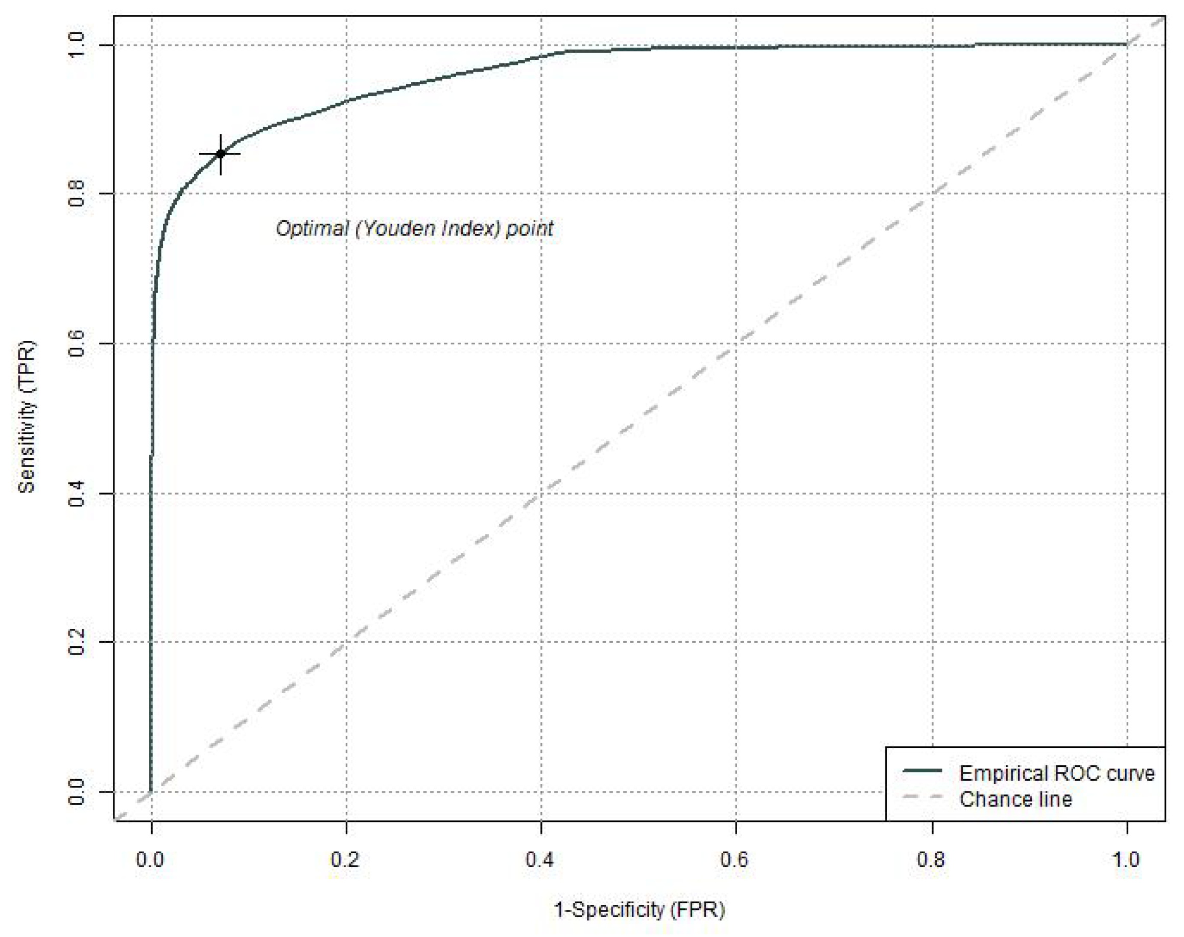
For instructional purposes, we display a ROC curve in Figure 3 which was created using the average OD as predictor with a sample size of n = 2 . The Youden index which is chosen as optimal cutoff value for the separation of “resistant” and “susceptible” is the average OD value that maximises the difference between TPR and FPR. It is also the point of the curve that is most distant from the chance line. Its value in this example is 0.77 which, however, cannot be deduced from the graph. At the Youden index, F P R = 0.052 , T P R = 0.844 and A U C = 0.96 .
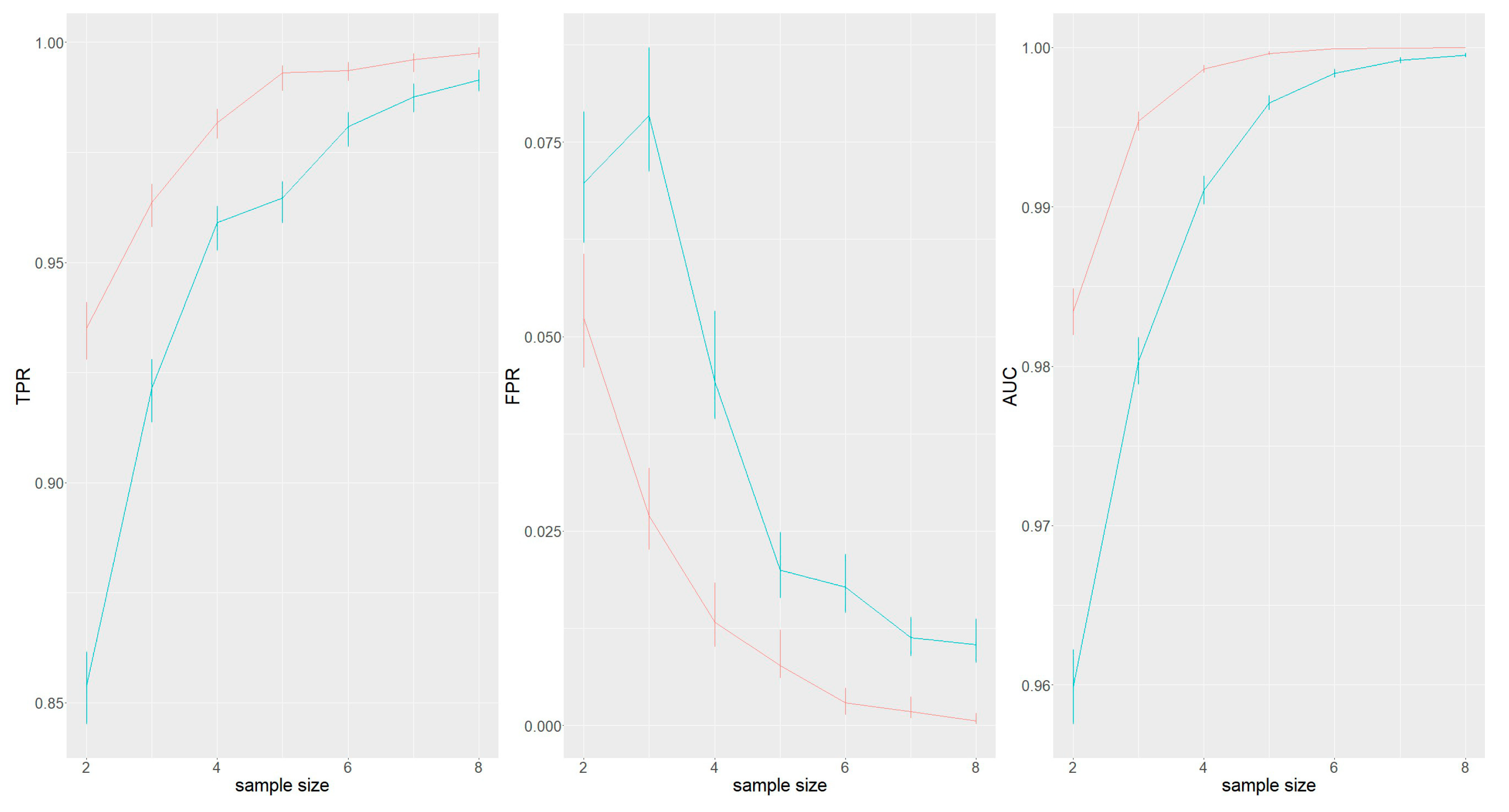
Figure 4 displays the TPR, FPR and AUC for each sample size with the average OD and Bayes factor as predictors. One can see that for each of the analysed sample sizes the TPR value based upon the Bayes factor is greater than the TPR value based upon the average OD as predictor. Analogously, the FPR based upon the Bayes factor is smaller for each sample size. Moreover, the AUC values based upon the Bayes factor is higher than the AUC based upon the average OD for each sample size. At a sample size of six, the AUC value based upon the Bayes factor as predictor has practically converged to one.
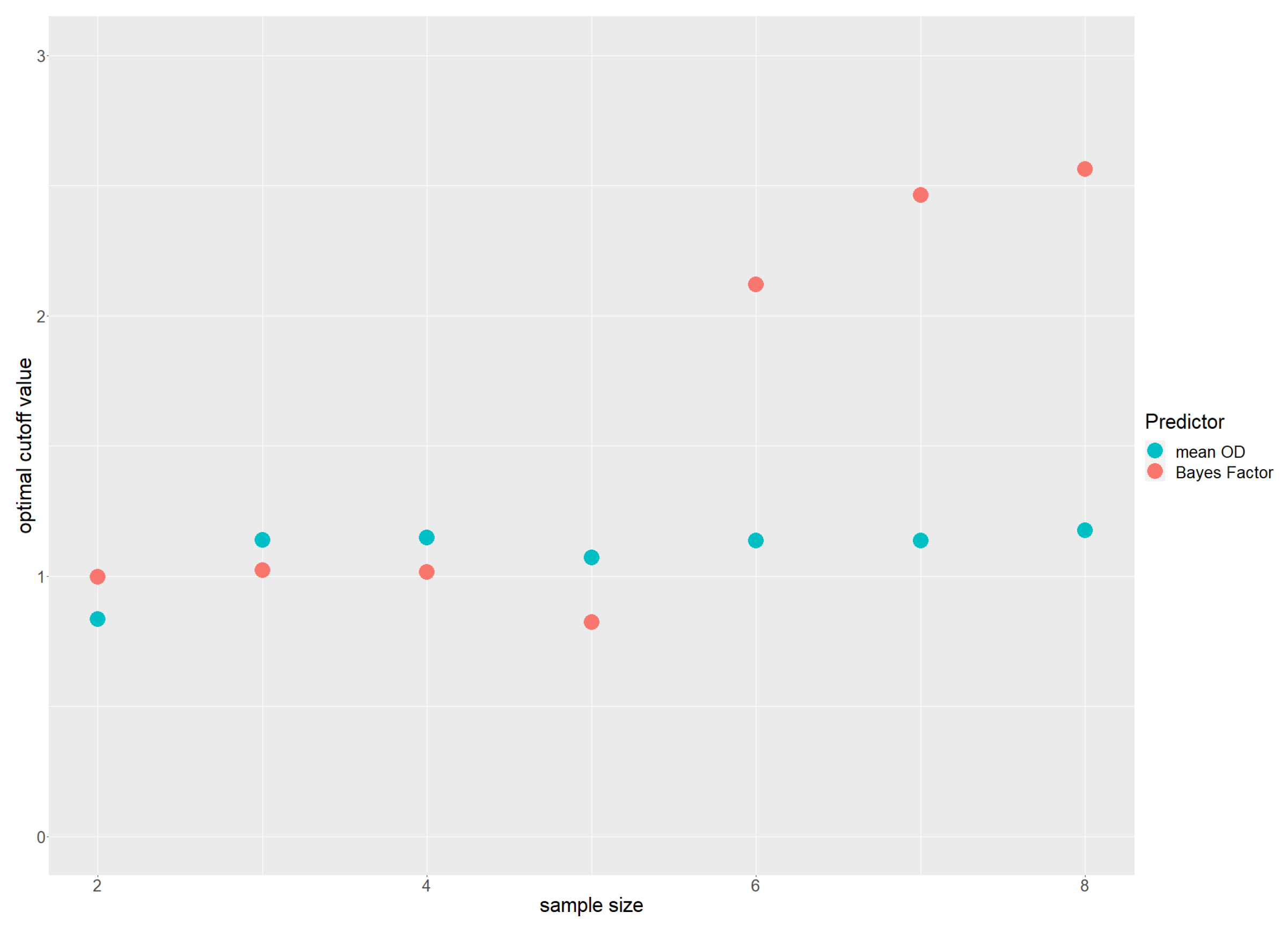
Figure 5 shows the optimal cutoff values for the mean OD and the Bayes factor for the sample sizes under investigation. The optimal cutoff values for the mean OD are relatively stable at around one as one also might have estimated from the distributions for the resistant and the susceptible pool shown in Figure 2. Values between 0.6 and 1.0 appear to be a good choice since an overwhelming fraction of all measurements from the resistant pool are below this range. The optimal cutoff for the Bayes factor is also in the range of one for samples sizes two to five, as one might expect given the theoretical value is 1.0. The divergent values for samples sizes six to eight ranging from 2 to 2.5 are less obvious. Plotting TPR against possible cutoff values between 1 and 10 revealed that they were above 0.99 in this range, such that the decision of the algorithm might depend on tiny numerical effects. The choice of the theoretical value of one as the optimal cutoff for Bayes factors, thus, seems to be justified also for practical purposes such that an ROC analysis does not seem to be absolutely necessary if one chooses Bayes factors as predictors.
Moreover, we applied both methods in a realistic setting. Therefore, we defined OD values from KWS C (74 measurements) to be the resistant training set, OD values from KWS F (86 measurements) to be the susceptible training set, and OD values from KWS D and KWS E were used as test sets. As a result, applying the mean OD as cutoff, 6 of the 10 KWS D samples were correctly classified as resistant, and 16 of the 19 KWS E samples were correctly classified as susceptible. Choosing the Bayes factor as predictor, 8 of the 10 KWS D samples were correctly classified as resistant, and 17 of the 19 KWS E samples were correctly classified as susceptible. These anecdotal calculations as examples confirm the superiority of the Bayes factor as predictor.
In order to facilitate the calculations for interested researchers and breeders, we make an R-script named classifyELISA.r freely available as a Supplementary file. The script reads in a file (TrainingSet.txt) containing the OD measurements that are labelled with either “resistant” or “susceptible”. Empirical density functions are calculated from which 10,000 small samples are drawn. The size of the small samples is the same as in the file of data to be classified (DataSet.txt). Both input files are also made available. After the calculation of sample means and Bayes factors for each small sample, optimal cutoff values are determined in a ROC analysis for both mean OD values and Bayes factors. These cutoff values are applied to classify the new data set provided in the file DataSet.txt. The results are written in the file PredictionSet.txt.

4. Discussion and Conclusions

We have shown in a simulation study that if a representative training set containing absorbance readings from ELISA together with a reliably assigned class label is available, small samples can be classified quite accurately. In more detail, our endeavours were two-fold. First, we wanted to improve a very simple decision procedure in which the average of few values is taken and compared to some conventional threshold, e.g., an average OD of 0.5. If the sample average is below this cutoff, the corresponding genotype is considered as resistant and is selected for further breeding towards rhizomania resistance. Otherwise, it is rejected. We have shown that in a ROC analysis the choice of the cutoff can be optimised in the sense that for it the distance between false positive and true positive rate is maximised. This simple decision strategy yielded surprisingly good results even for samples of size n = 2 (FPR = 0.07, TPR = 0.85).
Secondly, we calculated the Bayes factor for each sample based upon the empirical density functions that were derived from the training set and used it as predictor in a further ROC analysis. We found that the Bayes factor is a predictor that is superior to the average OD value for all sample sizes under investigation. Using the Bayes factor as a predictor, a TPR over 0.99 and a FPR below 0.01 can be expected for n 5 . This performance would be achieved with the average OD strategy only for n 8 .
Given that the calculation of the Bayes factor is relatively straightforward, applying the decision strategy based upon the Bayes factor could contribute to improving the selection procedure in corporate or academic settings by 3 to 4 percentage points in TPR and FPR for n = 3 with the advantage becoming less pronounced for larger samples.
We anticipate that our deliberations can be transferred to similar settings where binary decisions have to be made based upon small samples given approximate distributions of measurements in the two classes. Possible knowledge about the occurrence of the two classes could be considered by specifying prior probabilities in the Bayes factors.

Supplementary Materials

The following are available online at https://www.mdpi.com/article/10.3390/agriculture11100956/s1: Script S1: classifyELISA.r, R script for classification of small samples of OD values into resistant or susceptible. Table S2: TrainingSet.txt, table of three columns to estimate the optimal cutoff values. Column 1 contains identifiers, column 2 contains measurements, column 3 contains true labels. Table S3: DataSet.txt, data set of small samples as an example of measurements to be classified. Column 1 contains identifiers, column 2 contains measurement 1, column 3 contains measurement 2, column 4 contains measurement 3.

Author Contributions

A.O.S. conceptualised the study and created the R script. T.M.L., M.W., L.B. and A.O.S. wrote the manuscript. F.K.-O. planned the greenhouse trial and revised the manuscript. H.K. supervised the greenhouse trial and laboratory work and revised the manuscript. All authors have read and agreed to the published version of the manuscript.

Funding

The publication cost of this work was covered by the publication fund of the Göttingen State and University Library.

Institutional Review Board Statement

Not applicable.

Informed Consent Statement

Not applicable.

Data Availability Statement

Two data sets of fictional values are available as supplementary Tables S2 and S3 as example input for the script classifyELISA.r.

Acknowledgments

We thank T. Kneib (Center for Statistics, University of Göttingen) and W. Beyer (KWS SAAT SE & Co. KGaA) for valuable advice. Moreover, we would like to thank the Phytopathology group of KWS SAAT SE & Co. KGaA, most of all A. Ebeling and J. Gersch for performing the greenhouse trial and laboratory work.

Conflicts of Interest

The authors declare no conflict of interest.

Abbreviations

The following abbreviations are used in this manuscript:
AUCArea under the curve
BNYVVBeet necrotic yellow vein virus
DAS-ELISADouble antibody sandwich-ELISA
ELISAEnzyme-linked immunosorbent assay
FPRFalse positive rate
ODOptical density
ROCReceiver operation characteristic
TAS-ELISATriple antibody sandwich-ELISA
TPRTrue positive rate

References

  1. Canova, A. On the pathology of sugar beet. Inf. Fitopatol. 1959, 9, 390–396. [Google Scholar]
  2. Tamada, T.; Baba, T. Beet necrotic yellow vein virus from rizomania-affected sugar beet in Japan. Jpn. J. Phytopathol. 1973, 39, 325–332. [Google Scholar] [CrossRef]
  3. Fujisawa, I.; Sugimoto, T. Transmission of beet necrotic yellow vein virus by Polymyxa betae. Jpn. J. Phytopathol. 1977, 43, 583–586. [Google Scholar] [CrossRef]
  4. Rush, C.M. Ecology and Epidemiology of Benyviruses and Plasmodiophorid Vectors. Annu. Rev. Phytopathol. 2003, 41, 567–592. [Google Scholar] [CrossRef]
  5. Tamada, T.; Kondo, H. Biological and genetic diversity of plasmodiophorid-transmitted viruses and their vectors. J. Gen. Plant Pathol. 2013, 79, 307–320. [Google Scholar] [CrossRef]
  6. McGrann, G.R.D.; Grimmer, M.K.; Mutasa-Göttgens, E.S.; Stevens, M. Progress towards the understanding and control of sugar beet rhizomania disease. Mol. Plant Pathol. 2009, 10, 129–141. [Google Scholar] [CrossRef]
  7. Özmen, C.Y.; Khabbazi, S.D.; Khabbazi, A.D.; Gürel, S.; Kaya, R.; Oğuz, M.Ç.; Turan, F.; Rezaei, F.; Kibar, U.; Gürel, E.; et al. Genome composition analysis of multipartite BNYVV reveals the occurrence of genetic re-assortment in the isolates of Asia Minor and Thrace. Sci. Rep. 2020, 10, 1–11. [Google Scholar]
  8. Daly, D.; White, A.M.; Varnum, S.M.; Anderson, K.K.; Zangar, R.C. Evaluating concentration estimation errors in ELISA microarray experiments. BMC Bioinform. 2005, 6, 17. [Google Scholar] [CrossRef] [Green Version]
  9. Amiri, R.; Moghaddam, M.; Mesbah, M.; Sadeghian, S.Y.; Ghannadha, M.R.; Izadpanah, K. The inheritance of resistance to beet necrotic yellow vein virus (BNYVV) in B. vulgaris subsp. maritima, accession WB42: Statistical comparisons with Holly-1-4. Euphytica 2003, 132, 363–373. [Google Scholar] [CrossRef]
  10. Pferdmenges, F.; Korf, H.; Varrelmann, M. Identification of rhizomania-infected soil in Europe able to overcome Rz1 resistance in sugar beet and comparison with other resistance-breaking soils from different geographic origins. Eur. J. Plant Pathol. 2008, 124, 31–43. [Google Scholar] [CrossRef]
  11. Safar, S.; Bazrafshan, M.; Khoshnami, M.; Behrooz, A.A.; Hedayati, F.; Maleki, M.; Mahmoudi, S.B.; Malboobi, M.A. Field evaluation for rhizomania resistance of transgenic sugar beet events based on gene silencing. Can. J. Plant Pathol. 2020, 43, 179–188. [Google Scholar] [CrossRef]
  12. Wisler, G.; Lewellen, R.; Sears, J.; Liu, H.Y.; Duffus, J. Specificity of TAS-ELISA for beet necrotic yellow vein virus and its application for determining rhizomania resistance in field-grown sugar beets. Plant Dis. 1999, 83, 864–870. [Google Scholar] [CrossRef] [PubMed]
  13. Wisler, G.; Lewellen, R.; Sears, J.; Wasson, J.; Liu, H.Y.; Wintermantel, W. Interactions between Beet necrotic yellow vein virus and Beet soilborne mosaic virus in sugar beet. Plant Dis. 2003, 87, 1170–1175. [Google Scholar] [CrossRef] [Green Version]
  14. Broccanello, C.; McGrath, J.M.; Panella, L.; Richardson, K.; Funk, A.; Chiodi, C.; Biscarini, F.; Barone, V.; Baglieri, A.; Squartini, A.; et al. A SNP mutation affects rhizomania-virus content of sugar beets grown on resistance-breaking soils. Euphytica 2017, 214. [Google Scholar] [CrossRef]
  15. Giunchedi, L.; Biaggi, M.D.; Pollini, C.P. Correlation between tolerance and Beet necrotic yellow vein virus in Sugar-beet genotypes. Phytopathol. Mediterr. 1987, 26, 23–28. [Google Scholar]
  16. Capistrano-Gossmann, G.G.; Ries, D.; Holtgräwe, D.; Minoche, A.; Kraft, T.; Frerichmann, S.; Soerensen, T.R.; Dohm, J.C.; González, I.; Schilhabel, M.; et al. Crop wild relative populations of Beta vulgaris allow direct mapping of agronomically important genes. Nat. Commun. 2017, 8. [Google Scholar] [CrossRef] [PubMed]
  17. Clark, M.F.; Adams, A.N. Characteristics of the Microplate Method of Enzyme-Linked Immunosorbent Assay for the Detection of Plant Viruses. J. Gen. Virol. 1977, 34, 475–483. [Google Scholar] [CrossRef]
  18. Fecker, L.F.; Koenig, R.; Obermeier, C. Nicotiana benthamiana plants expressing beet necrotic yellow vein virus (BNYVV) coat protein-specific scFv are partially protected against the establishment of the virus in the early stages of infection and its pathogenic effects in the late stages of infection. Arch. Virol. 1997, 142, 1857–1863. [Google Scholar]
  19. Lottspeich, F.; Engels, J.W. Bioanalytik; Spektrum: Heidelberg, Germany, 2012. [Google Scholar]
  20. Biaggi, M.D.; Stevanato, P.; Trebbi, D.; Saccomani, M.; Biancardi, E. Sugar Beet Resistance to Rhizomania: State of the Art and Perspectives. Sugar Tech. 2010, 12, 238–242. [Google Scholar] [CrossRef]
  21. De Biaggi, M. Méthodes de sélection—Un cas concret. In Proceedings of the IIBR 50th Winter Congress of the International Institute for Sugar Beet Research (IIBR), Brussels, Belgium, 11–12 February 1987; Institut International de Recherches Betteravières: Brussels, Belgium, 1987. [Google Scholar]
  22. Büttner, G.; Märländer, B.; Manthey, R. Breeding for resistance to rhizomania in sugar-beet (Beta vulgaris L.). Plant Breed. 1995, 114, 160–164. [Google Scholar] [CrossRef]
  23. Hoijtink, H.; Mulder, J.; van Lissa, C.; Gu, X. A tutorial on testing hypotheses using the Bayes factor. Psychol. Methods 2019, 24, 539. [Google Scholar] [CrossRef] [Green Version]
  24. Goodman, S.N. Toward evidence-based medical statistics. 2: The Bayes factor. Ann. Intern. Med. 1999, 130, 1005–1013. [Google Scholar] [CrossRef]
  25. Wade, P.R. Bayesian methods in conservation biology. Conserv. Biol. 2000, 14, 1308–1316. [Google Scholar] [CrossRef] [Green Version]
  26. Evans, R.B.; Erlandson, K. Robust Bayesian prediction of subject disease status and population prevalence using several similar diagnostic tests. Stat. Med. 2004, 23, 2227–2236. [Google Scholar] [CrossRef] [PubMed]
  27. Hanson, T.E.; Johnson, W.O.; Gardner, I.A.; Georgiadis, M.P. Determining the infection status of a herd. J. Agric. Biol. Environ. Stat. 2003, 8, 469–485. [Google Scholar] [CrossRef]
  28. Kass, R.E.; Raftery, A.E. Bayes Factors. J. Am. Stat. Assoc. 1995, 90, 773–795. [Google Scholar] [CrossRef]
  29. Morisawa, J.; Otani, T.; Nishino, J.; Emoto, R.; Takahashi, K.; Matsui, S. Semi-parametric empirical Bayes factor for genome-wide association studies. Eur. J. Hum. Genet. 2021, 29, 800–807. [Google Scholar] [CrossRef]
  30. Van Hulzen, K.; Schopen, G.; van Arendonk, J.; Nielen, M.; Koets, A.; Schrooten, C.; Heuven, H. Genome-wide association study to identify chromosomal regions associated with antibody response to Mycobacterium avium subspecies paratuberculosis in milk of Dutch Holstein-Friesians. J. Dairy Sci. 2012, 95, 2740–2748. [Google Scholar] [CrossRef] [PubMed] [Green Version]
  31. Paul, H.; Henken, B.; Alderlieste, M. A greenhouse test for screening sugar-beet (Beta vulgaris) for resistance to beet necrotic yellow vein virus (BNYVV). Neth. J. Plant Pathol. 1992, 98, 65–75. [Google Scholar] [CrossRef]
  32. R Core Team. R: A Language and Environment for Statistical Computing; R Foundation for Statistical Computing: Vienna, Austria, 2020. [Google Scholar]
  33. Wickham, H. ggplot2: Elegant Graphics for Data Analysis; Springer: New York, NY, USA, 2016. [Google Scholar]
  34. Sarkar, D. Lattice: Multivariate Data Visualization with R; Springer: New York, NY, USA, 2008; ISBN 978-0-387-75968-5. [Google Scholar]
  35. Kooperberg, C. Logspline: Routines for Logspline Density Estimation. Version: 2.1.16. 2020. Available online: https://cran.r-project.org/web/packages/logspline/index.html (accessed on 1 September 2021).
  36. Kooperberg, C.; Stone, C.J. Logspline density estimation for censored data. J. Comput. Graph. Stat. 1992, 1, 301–328. [Google Scholar]
  37. Khan, R.A.; Brandenburger, T. ROCit: Performance Assessment of Binary Classifier with Visualization. Version: 2.1.1. 2019. Available online: https://cran.r-project.org/web/packages/ROCit/index.html (accessed on 1 September 2021).
  38. Peter, E. fbroc: Fast Algorithms to Bootstrap Receiver Operating Characteristics Curves. Version: 0.4.1. 2019. Available online: https://cran.r-project.org/web/packages/fbroc/index.html (accessed on 1 September 2021).
  39. Robin, X.; Turck, N.; Hainard, A.; Tiberti, N.; Lisacek, F.; Sanchez, J.C.; Müller, M. pROC: An open-source package for R and S+ to analyze and compare ROC curves. BMC Bioinform. 2011, 12, 1–8. [Google Scholar] [CrossRef] [PubMed]
Figure 1. Histograms of optical density (OD) values for each of the six sugar beet genotypes. The X axis represents OD values in the range from 0 to 4 with a binning width of 0.1. The Y axis represents percentage of measurements in each bin.
Agriculture 11 00956 g001
Figure 2. Histograms of optical density (OD) values for the two pools of resistant (left) and susceptible (right) genotypes. The X axis represents OD values in the range from 0 to 4 with a binning width of 0.1. The Y axis represents percentage of measurements in each bin.
Agriculture 11 00956 g002
Figure 3. Exemplary receiver operating characteristic (ROC) curve for a sample size of n = 2 . The Youden index which is the point of the curve that is most distant from the chance line is the average OD value that maximises the difference between TPR and FPR.
Agriculture 11 00956 g003
Figure 4. True positive rate (TPR) (left), false positive rate (FPR) (middle), and area under the curve (AUC) (right) are given as a function of the sample size n for average OD (green) and Bayes factor (red) as predictors.
Agriculture 11 00956 g004
Figure 5. The optimal cutoff values are shown for the predictors average OD value (green) and Bayes factor (red).
Agriculture 11 00956 g005
Publisher’s Note: MDPI stays neutral with regard to jurisdictional claims in published maps and institutional affiliations.