Article

Sources of Total-Factor Productivity and Efficiency Changes in China’s Agriculture

1
School of Economics, Shandong University of Finance and Economics, Shandong Province, Jinan 250014, China
2
Faculty of Economics, Chiang Mai University, Chiang Mai 50200, Thailand
3
Plymouth Business School, University of Plymouth, Drake Circus, Plymouth PL4 8AA, UK
*
Author to whom correspondence should be addressed.
Agriculture 2020, 10(7), 279; https://doi.org/10.3390/agriculture10070279
Submission received: 22 May 2020 / Revised: 18 June 2020 / Accepted: 6 July 2020 / Published: 8 July 2020
(This article belongs to the Special Issue Productivity, Efficiency, and Sustainability in Agriculture)

Abstract

:
The core of agricultural development depends on agricultural production efficiency improvement, and total-factor productivity growth is its significant embodiment. Hence, it is essential to address the question of “how to improve China’s agricultural productivity and efficiency in order to achieve growth and sustainability of agriculture in the future”. This paper estimates indices of China’s agricultural technical efficiency (TE) scores, total-factor productivity (TFP), and its two components, technological change/progress (TC) and technical efficiency change (EC), using provincial-level panel data of 30 provinces from 2002 to 2017 by applying a stochastic frontier approach (SFA). The paper also identifies determinants of TE, TC, and TFP using selected indicators from four hierarchical levels of the economy, i.e., farm level, production environment level, provincial level, and the state level, by applying a system-GMM method. Results reveal that agricultural labor, machinery, agricultural plastic film, and pesticides are the significant drivers of agricultural productivity, with no significant role of land area under cultivation. Constant returns to scale exist in China’s agriculture. The agricultural technical efficiency level fluctuated between 80% and 91% with a stable trend and a slight decline in later years, while TFP improved consistently over time, mainly driven by technological progress. Among the determinants, government investment in agricultural development projects significantly drives TC and TE, while the experienced labor force significantly increases TE. The disaster rate significantly reduces TE but promotes TC and TFP. The literacy rate significantly improves TC and TFP. However, government expenditures in “agriculture, forestry, and water” significantly reduce TE, TC, and TFP. Policy recommendations include (1) increased levels of mechanization and agriculture film use while avoiding an increase in pesticide use, (2) a continued increase in government expenditure in agricultural development projects, R&D to improve technological progress, and diffusion of modern agricultural technologies, and (3) investment in education targeted at the farming population in order to continue the growth in the productivity and sustainability of China’s agriculture.

1. Introduction

Agriculture is the primary source of food production for human society and a foundation of national economic development [1], especially for developing economies. As the largest developing country in the world, the Chinese government attaches great importance to the development of its agricultural sector. Since the reform and opening-up of the economy, China’s total agricultural output has increased rapidly [2]. Intensive use of inputs is believed to be behind such rapid growth in output. As China’s economic development entered a new phase, the traditional growth model became more and more unsustainable because of its reliance on the increased use of agricultural factor inputs [3]. The key to solving such a high reliance on input increase is to improve agricultural productivity [4]. Furthermore, raising agricultural productivity level could, to some extent, make-up for the shortage of resources due to a large population base with relatively little arable land and water, along with the acceleration of agricultural modernization. Therefore, the key elements of agricultural productivity growth are TC, EC, and growth in tTFP [5]. The modern economic growth theory shows that long-term economic growth should mainly rely on technical progress and TFP improvement, and so should agricultural growth [6]. Thus, the driving force of China’s agricultural development should shift from conventional factor input growth to improvements of TC and TFP, which are also the current main goals of the Chinese government. This is because improvements in productivity and efficiency, along with agricultural modernization, are considered as the decisive factors for the sustainable development of China’s agriculture in the future.

1.1. Chinese Agricultural Technology Efficiency

Due to the importance of agriculture in developing countries, research into enhancing agricultural production has drawn significant attention from academia. Many scholars have conducted profound research on EC and TFP growth in agriculture from various perspectives. Farrell [7] pioneered the research on production efficiency and put forward the measurement method of agricultural production efficiency. Rahman and Barmon [8], using the stochastic frontier analysis method, conducted an analysis of agricultural technical efficiency in Bangladesh and reported that the mean technical efficiency score in rice production was very high at a 90% level. Kawagoe et al. [9] estimated an aggregate agricultural production function using cross-country data from 1960, 1970, and 1980 and compared agricultural productivity between developed and less-developed countries. They reported that agriculture is characterized by increasing returns in developing countries, but constant returns in less developed countries and unfavorable population/land ratios are not a direct obstacle to rapid agricultural development. Chen and Song [10] used county-level data to analyze the agricultural technology gap and the efficiency gap between different regions in China and found the existence of large gaps across regions. Agricultural technical efficiency was the highest in the eastern part, whereas the technology level was the highest in the northeast of China. Based on the panel data of 30 provinces in China from 2001 to 2012, Yin and Wang [11] found that agricultural technical efficiency has shown a rising tendency in China. In contrast, Li and Zhang [12] and Mao and Koo [13] found that China’s agricultural production has faced a problem of low technical efficiency and noted that China has a great potential to improve agricultural productivity by improving technical efficiency in the future. To sum up, it seems that there is no consensus on the conclusion regarding agricultural technical efficiency changes in China, and the estimated technical efficiency scores vary largely due to differences in data, selection of provinces, data periods, and application of different research methods.

1.2. Chinese Agricultural Total-Factor Productivity

Research on agricultural TFP also received a high level of attention across the board. Barath and Ferto [14] studied relative productivity levels of European agriculture between 2004 and 2013 and decomposed productivity changes. They reported that the European TFP declined slightly, with significant differences across member states during the analysis period. Rahman and Salim [15] studied TFP indices for agriculture in 17 regions of Bangladesh using data from 1948. They applied the Fare–Primont index and decomposed the TFP index into six finer components of technical change, technical-, scale- and mix-efficiency changes, and residual scale- and residual mix-efficiency changes. They reported continued growth in TFP, driven mainly by technological progress, with some regions leading in growth performance. Song et al. [16] used the panel data of 31 provinces in China from 1999 to 2008 and measured changes of TFP of agricultural production in China using the Malmquist productivity index and the bootstrapped Malmquist productivity index. They reported that agricultural TFP increased annually by 6.1% from 1999 to 2008, with obvious fluctuations in the different periods. Tian and Yu [17] noted that the annual growth rate of TFP was 2.03% in China’s agricultural sector from 1950 to 2008. Shen et al. [18], using the accumulative and complete Luenberger–Hicks–Moorsteen TFP index, analyzed changes in agricultural TFP from 1997 to 2015 in China. The results revealed that there were large differences in China’s agricultural TFP growth and its components at different times and across different provinces in China. As with the case of agricultural TE, it seems that the results on China’s agricultural TFP have variable outcomes.

1.3. Factors Influencing Agricultural Total-Factor Productivity and Technical Efficiency

Scholars have also conducted studies on the influencing factors of TFP and TE of the agricultural sector. Andersen [19] studied the relationship between public investment in agricultural R&D, productivity growth, and the resulting economic benefits generated using American data from 1949 to 2002. Empirical results showed that public investment in agricultural R&D had a positive economic return. Yan et al. [20], using a selection of the Chinese household tracking survey data of 2012, conducted an empirical study on the relationship between farm size and agricultural production efficiency by using the SFA method and found that there is an inverted “U”-shaped relationship between farm size and output. Zeng et al. [21] studied the impact of land consolidation measures implemented in China on the agricultural TE using the SFA method. Results revealed that land consolidation promoted the transfer of land-use rights and indirectly improved nonagricultural employment, thus improved the agricultural TE of producers. Grashuis reviewed the empirical literature on agricultural cooperatives and found that agricultural cooperatives had a huge positive impact on the members’ agricultural production activities [22]. Bahta et al. [23] found significant effects of family size, human capital, and other factors on the agricultural TE of small farmers. Although a lot is known from these studies about the drivers of agricultural production and/or agricultural TE, most of these research studies are based on cross-sectional data.
Based on the aforementioned review, it is clear that a lot of attention has been paid to estimating agricultural TE and agricultural productivity and their influencing factors in various parts of the world, including China. However, there are issues related to the consensus that are related to the measures of agricultural TE and agricultural productivity changes and their influencing factors. Most authors have used cross-sectional data, and if panel data is used, the length and coverage of the panel are limited in time. Therefore, it is important to study changes in TFP and TE and their factors influencing China’s agricultural sector with higher coverage of provinces, including longer panel data covering the years 2002–2017, by applying an appropriate parametric approach.
Given this backdrop, the specific objectives of this study are to (a) estimate agricultural TE of 30 provinces in China, (b) measure TFP change of 30 provinces in China, and (c) identify factors influencing changes in TE, TC, and TFP over time in China. The contribution of the present study to the existing literature is as follows. First, it estimates the indices of agricultural TE, TC, EC, and TFP of 30 provinces, covering a longer time-period by using a parametric procedure. The advantage of a parametric approach is that it is capable of separating statistical noise and measurement errors from the TE scores. Second, the determinants of TE, TC, and TFP are identified jointly by applying a system-GMM estimation method. Third, indicators of these determinants are selected from four hierarchical levels, i.e., farm level, production environment level, provincial level, and the state level. Fourth, the study puts forward corresponding policy recommendations specifically for improving agricultural production, TFP, TC, and TE, which is conducive to realizing sustainable and sound development of China’s agriculture in the future.
This article has the following structure: The next section presents the research method, including model building and data selection. Section 3 presents the results of the empirical analysis, and Section 4 provides the conclusions and policy recommendations.

2. Research Method

2.1. Model Building

The stochastic frontier model was proposed by Aigner, Lovell, and Schmidt [24] and Meeusen and van Den Broeck [25]. Following Kumbhakar and Lovell [26], the form of a standard SFA model can be expressed as follows:
Y i t = f ( x i t , t ) · exp ( v i t u i t )
where Y i t represents total agriculture output value at period t in province i , f ( x i t , t ) denotes the agricultural production frontier, x i t represents the agricultural input factor in province i at time t for time trend. vit represents a two-sided random error, accounting for measurement and statistical errors; uit ≥ 0 denotes a non-negative technical inefficiency variable, measuring the difference between actual agricultural output Y i t and the maximum agricultural output f ( x i t , t ) possible under the given technology level. Greene [27] noted that if observations on uit and vit are independent over time, as well as across individuals, then the panel nature of the data set is irrelevant. Therefore, based on this premise, we apply the pooled data for analysis under a cross-sectional setting, as done in Coelli et al. [28]. We consider all four major potential distributional forms of the technical inefficiency variable based on the literature. These are half-normal distribution [24], exponential distribution [25], truncated normal distribution [29], and gamma distribution [30], respectively, while maintaining the assumption of independence between v i t and u i t .
Taking the natural log of both sides of Equation (1) provides
L n y i t = L n f ( x i t , t ) + v i t u i t
With reference to Coelli and Rahman [28], uit shows technical efficiency in period t in province i. When u i t = 0 and TE = 1, this indicates that agricultural production is on the frontier, and there is no technical inefficiency in this province. When u i t 0 and TE < 1, this indicates that agricultural production is below the frontier, and there is technical inefficiency in this province.
T E i t = E [ exp ( u i t ) | ( v i t u i t ) ]
The technical efficiency change index (EC) from period t to period s (s = t − 1) in province i is given by
E C i t = T E i t / T E i s
The TE scores were computed from the estimated parameters of the stochastic frontier model. The technological change between period t and period s is given by
T C i t = { [ 1 + f ( x is , s ) s ] × [ 1 + f ( x it , t ) t ] } 0.5
The product of ECit and TCit provides the Malmquist TFP index as follows (Coelli and Rahman, 2003):
T F P i t = E C i t T C i t
To explore the determinants of TFP and TC, Chen and Song [10] and Coelli and Rahman [28] established several regression models to investigate the determinants of TFP and its components. However, regression conducted independently for any one component at a time ignores the correlation between equations. Yin and Wang [11] and Ali et al. [31] used panel data with the OLS method to analyze the influence factors of TFP but ignored endogeneity, which may also lead to biased and inconsistent estimation [32]. Thus, in our determinant analysis, in addition to allowing for correlations between equations, we have also considered the issue of potential endogeneity of regressors. To solve the endogeneity problems, instrumental variable (IV) class estimators and generalized method of moments (GMM) estimators are often used. In contrast to traditional IV class estimators such as 2SLS and 3SLS, the GMM estimator uses a weighting matrix and takes into account temporal dependence, heteroscedasticity, or autocorrelation [33,34]. Therefore, the system generalized method of moments (SYS-GMM) estimator in panel data models was applied to explain the sources of TFP and its components in China, which account for both the correlation across equations and the endogeneity of regressors. The system of equations can be expressed as
{ T E i t = α Z i t + ε 1 i t T C i t = δ Z i t + ε 2 i t T F P i t = ϕ Z i t + ρ T C i t + φ E C i t + ε 3 i t
where Z i t is the vector of explanatory variables for TE, TC and TFP; α , δ , and ϕ are the parameter vectors that represent the impact of the determinants; ρ and φ represent the coefficient of T C i t and E C i t ; ε 1 i t , ε 2 i t , and ε 3 i t represent random error terms of the system equations. The detailed explanations and proof of SYS-GMM estimators can be referred to in Blundell and Bond [35] and Carstensen and Toubal [36].
The empirical model is estimated by using the two-step estimation method of SFA. The first step is to estimate the parameters of the stochastic frontier model with different distributional assumptions of the inefficiency term in order to obtain the technical efficiency scores under each of the four models (i.e., Equation (3)). Then, the indices of TC, EC, and TFP are calculated using Equations (4)–(6). The second step is to use the system-GMM method to analyze the influence factors of TE, TC, and TFP. Although Wang and Schmidt [37] proved that the two-step estimation method provides a biased estimation of the determinants of technical efficiency, we still need to apply the two-step method because TFP, TC, and EC are derived variables, which cannot be obtained in a one-step estimation. These variables are computed after using the estimated TE scores from the estimation of the production function and coefficients of the time-trend and time-input variable interactions of the production function model to obtain TC scores. Furthermore, various current studies in literature, such as Iglesias et al. [38], Cao et al. [39], Song and Chen [40], and Moutinho et al. [41], have applied the two-step estimation method, implying that it is still widely used in academia. Thus, a two-stage estimation method is applied in this study, although we acknowledge that there is a limitation to this method.

2.2. Data and Variable Declaration

2.2.1. Variable Selection

The value of annual agricultural output at constant prices was used to represent the agricultural output of each province in China. Based on the existing related literature [10,15,28], the following inputs were selected: (1) labor, expressed by employed personnel in the primary industry of each province; (2) land, expressed by the sown area of farm crops in each province; (3) agricultural capital stock, expressed by the total horsepower of agricultural machinery; (4) pesticides, expressed by the amount of pesticide used in each province; (5) agricultural plastic film, expressed by the amount of agricultural plastic film used in each province. We also added a time-trend variable to capture technological progress and trend-input variable interactions to compute the TC variable from the estimated parameters using Equation (5).

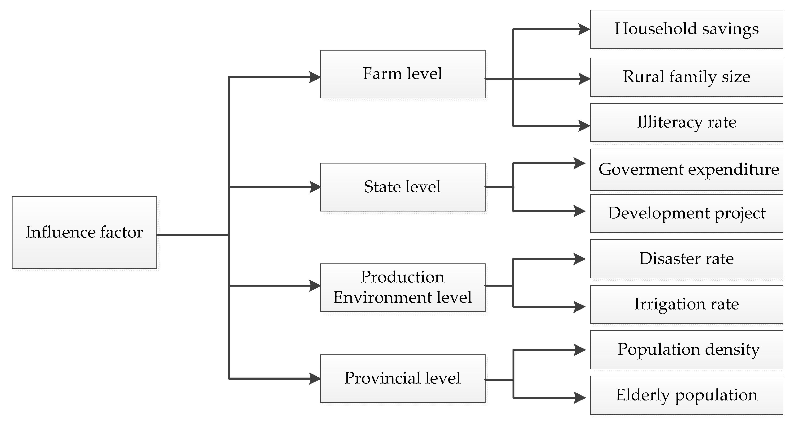
2.2.2. Construction of Variables Influencing TFP and Its Components

Ali et al. [31] found that family size had a significant impact on agricultural technical efficiency, while Chen and Song [10] believed that population density and available credit per capita had a significant impact on agricultural production efficiency. In this article, considering that there are few households with borrowing behaviors in China’s rural areas, we argue that household savings in China’s rural areas could have a greater impact on agricultural productivity than available credit per capita. O’Donoghue and Heanue [42] found that farmers’ education level had a significant impact on agricultural TE. Therefore, we have included family size, household savings, and illiteracy rate as indicators belonging to the farm-level hierarchy. Coelli and Rahman [28] found that agricultural production conditions, such as agricultural disaster rates, significantly affected TE and TFP. Therefore, agricultural disaster and irrigation rates were included as indicators belonging to the production-environment hierarchy. Rada and Schimmelpfennig [43] used Indian agricultural production and policy data for the period 1980–2008 to study agricultural TFP and its components and concluded that the government’s agricultural fiscal expenditure had an important impact on agricultural productivity. Rahman and Salim [15] also presented the same conclusion for Bangladesh agriculture. Therefore, we have used government expenditures on agriculture, forestry, and water and government investments in comprehensive agricultural projects in agriculture as indicators belonging to the state-level hierarchy. We also used the proportion of rural elderly population and population density as indicators belonging to the provincial-level hierarchy [44]. Indicators to identify determinants of TFP, TE, and EC are displayed in Figure 1.

2.2.3. Data Source

Data were compiled for 30 provincial regions in China, covering the period 2002 to 2017. Although China has 31 provinces, due to the lack of relevant data in Tibet, we selected 30 provinces as samples for this research. Therefore, the panel data contained 480 samples from 30 provinces for 16 consecutive years. The data were mainly from China Statistical Yearbooks (2003–2018), China Rural Statistical Yearbooks (2003–2018), China Population and Employment Statistical Yearbooks (2003–2018), and the National Bureau of Statistics of China (2003–2018).

2.2.4. Data Processing

The value of the annual agricultural output of each province measured at constant prices was taken as the agricultural output variable. Agricultural labor input was approximated by the number of primary industrial labor in each province. Data for the average household size of each province for 2002 was not available. Therefore, the number of the rural population was divided by the number of rural households of each province to obtain household size information for 2002. The savings of rural households in each province was calculated by multiplying per capita savings by the average population size of rural households of each province. The illiteracy rate was expressed as the ratio of the percentage of the rural illiterate/semiliterate population to the population aged 15 and over from China’s annual population sample survey data. The irrigation rate is the ratio of irrigated areas to crop-sown areas. Agricultural disaster rate is the ratio of agricultural disaster areas to crop-sown areas. The proportion of the elderly population was expressed as the ratio of the total rural population aged 65 years and over to the total rural population in each province, which was calculated on the basis of the data of China’s population sampling survey in each year. Since China conducted a census in 2010, the proportion of the elderly population in 2010 was calculated based on the census data. The population density was expressed as the number of people living in an average area of one square kilometer of each province. The centralized processing of the five variables, respectively, agricultural labor input, crop sown area, total power of agricultural machinery, agricultural plastic film usage amount, and pesticide usage amount, was conducted.

2.2.5. Descriptive Statistical Analysis

The descriptive statistics of the variables are presented in Table 1. The data show rising trends of agricultural output, crop-sown area, agricultural mechanization, and agricultural plastic film usage, a declining trend of labor input, and a first rising and then declining trend of pesticide usage, which are consistent with the actual situation observed in China.

2.2.6. Model Setup

A functional form is required to estimate the stochastic frontier production function. Commonly, Cobb–Douglas and/or translog functions are used. Chiang et al. [45] showed that the translog form could better fit the data and has flexible and elastic coefficients in general. Therefore, a translog stochastic frontier production function is specified, as shown in Equation (8):
L n y i t = β 0 + a = 1 5 β a L n x a i t + 1 2 ( a = 1 5 b = 1 5 β a , b L n x a i t L n x b i t ) + β 6 t + 1 2 β 7 t 2 + a = 1 5 β at t L n x a i t + ( v i t u i t )

3. Empirical Result Analysis

3.1. Estimated Results

Parameter estimation of the translog stochastic frontier production function was conducted using LIMDEP 9.0 (Econometric Software, New York, NY, USA) and STATA 14.0 (StataCorp, Texas, TX, USA) software, and the results are presented in Table 2. Models (1)–(4) represent various assumptions of the inefficiency variable u distributed as half-normal, exponential, truncated normal, and gamma distributions. In general, there is little difference in the model results under the four alternative distributional assumptions. However, from the point of AIC results, the half-normal distribution model has the minimum AIC. Thus, half-normal distribution is identified as the optimal model. The coefficient σ 2 = σ u 2 + σ v 2 is statistically significant at the 1% level of significance, indicating that the stochastic frontier model fitted the data better than the traditional production function. Based on the value of μ , one could determine whether there is any technical inefficiency effect. If λ = 0 , the gap between the production function and frontier is mainly due to the noise effect, instead of the existence of technical inefficiency. If λ is close to 1, it shows that all deviations from the frontier are due to the impact of technical inefficiency. The estimated result of the λ coefficient is 0.91 and it is significant at the 1% level, indicating that technical inefficiency in production exists in China’s agriculture and it is necessary to apply stochastic frontier model analysis. The model fit is quite good based on the Wald test-statistic and the value of the log likelihood function.
With reference to the model parameter estimates, the sum of the coefficients of agricultural labor input, crop-sown area, agricultural machinery, agricultural plastic film usage, and pesticide usage is close to 1, which satisfies the assumption of constant returns to scale, namely, that agricultural output increases at the same rate as an increase in agricultural labor, agricultural machinery, agricultural plastic film usage amount, and pesticide usage. An increase in agricultural labor input by 1% will increase agricultural output by 0.261%. Similarly, with an increase in agricultural machinery by 1%, agricultural output will increase by 0.104%. With an increase in the use of agricultural plastic film by 1%, agricultural output will increase by 0.341%. With an increase in pesticide use by 1%, agricultural output will increase in value by 0.350%. Therefore, it is clear that pesticide use has the highest impact, followed by agricultural plastic film, in increasing agricultural output, while land area has no significant impact, which is consistent with Badar’s conclusion [46]. The coefficient on the time-trend variable is positive and significant, indicating that there is technological progress. The frontier is shifting upwards at a rate of 0.20% per year (Coelli et al. 2003). Considering that the translog function violates regularity conditions, we have provided checks for regularity conditions, and the results of these checks are presented in Table 3. For all factor inputs, the following two conditions must be met: (1) monotonicity, i.e., positive marginal products, and (2) diminishing marginal productivity [47,48]. Calculation results demonstrate that the two restrictions hold for all the inputs, and therefore, our translog production frontier model does not violate regularity conditions.

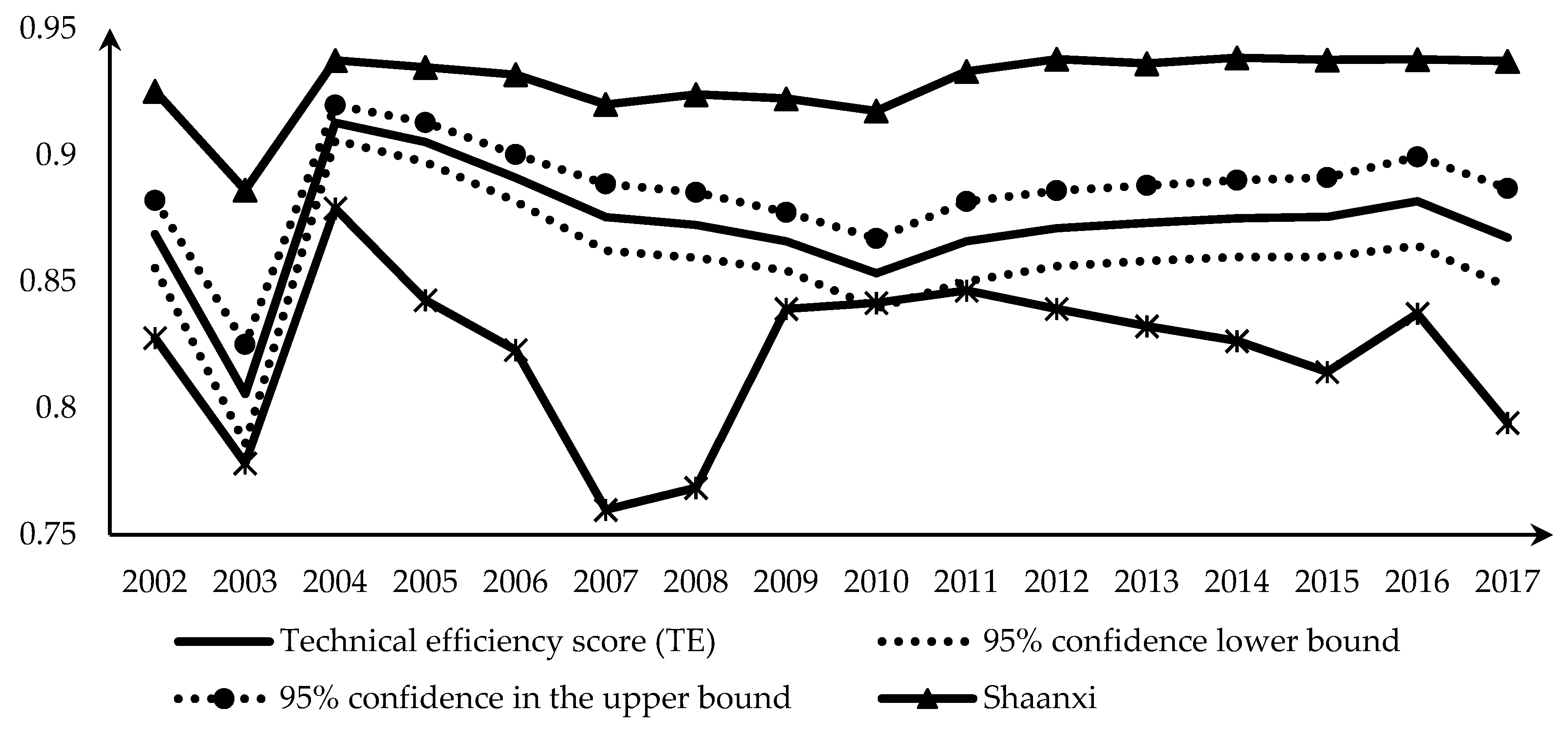
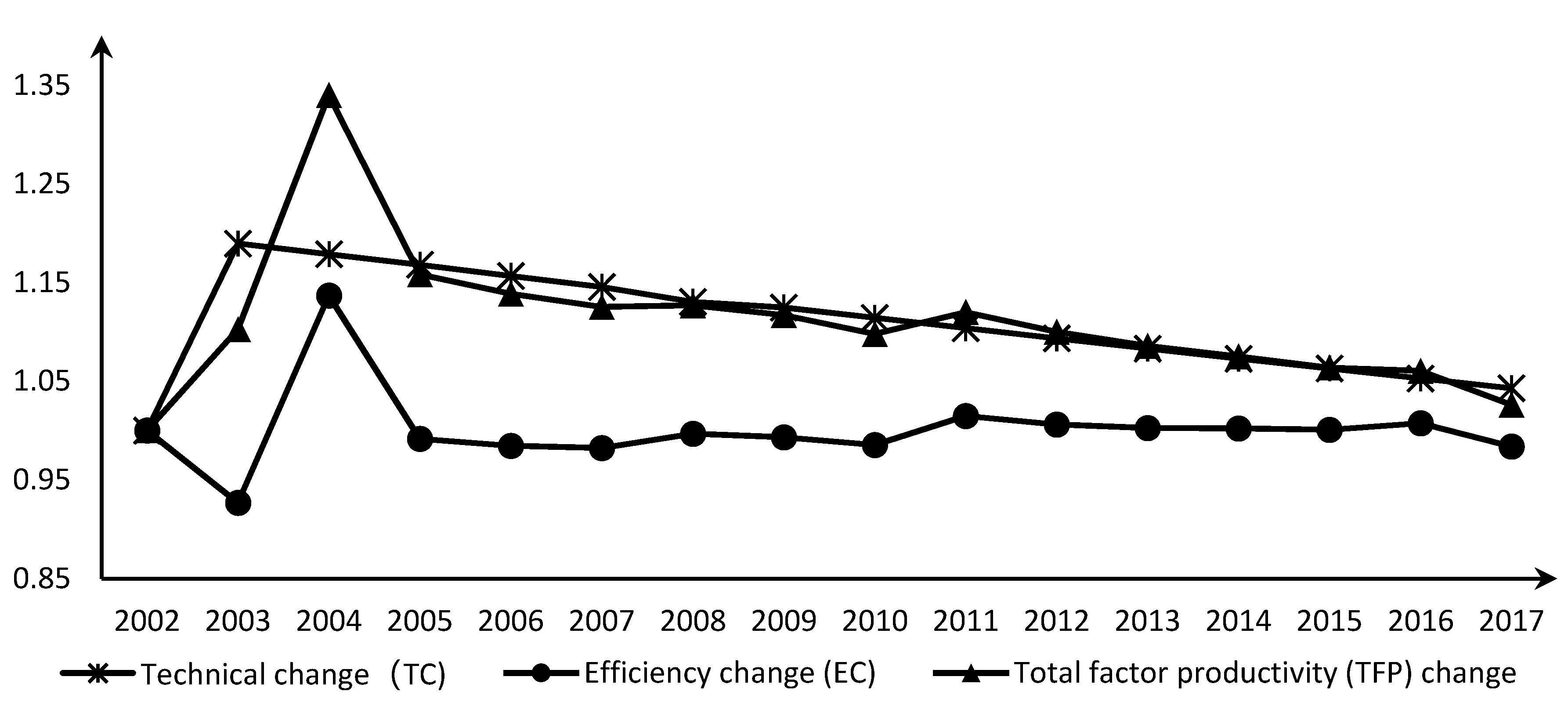
3.2. Total-Factor Productivity and Its Decomposition

According to Equations (3)–(6) and the parameter estimates of the stochastic frontier model (Equation (8)), we obtained indices of TE, TC, EC, and TFP in 30 provinces of China for the period 2002 to 2017. Table 4 shows the mean values of TE, TC, EC, and TFP for each province from 2002 to 2017. From the perspective of agricultural TE, the technical efficiency score, Taiyuan provincial capital of Shanxi province had the lowest average technical efficiency of 0.8219, and Xian provincial capital of Shaanxi province had the highest average technical efficiency of 0.9286. The TFP change index is greater than 1 in all provinces, indicating that the TFP increased in all provinces over time from 2002 to 2017. Similarly, the TC index is greater than 1 in each province, indicating that agricultural technology has progressed continuously in each province. The EC index ranges from 0.9892 to 1.0078, indicating that technical efficiency is little changed in each province and there are subtle differences among provinces. The conclusion is that the growth of agricultural TFP mainly came from the improvement in TC rather than EC in China. It is different from the development model of African agricultural growth, which has mainly relied on efficiency improvement [49].
The trend in the agricultural TE score from 2002 to 2017 is presented in Figure 2, including its 95% confidence interval. It is shown in Figure 2 that China’s agricultural TE score is mainly stable, with a slight decline in recent years and a sharp dip in 2003. The dip may have been due to the “SARS” epidemic in 2003. In 2004, with the end of the SARS epidemic, the Chinese government introduced policies to benefit farmers, such as reducing or exempting agricultural taxes and increasing agricultural subsidies, which led to the rapid progress of TE improvement, which was even higher than that in 2002. However, after 2004, the TE score showed a downward trend until 2010. From 2010 to 2016, the level of the agricultural TE score rose slowly, while in 2017, it showed a downward trend again. Shaanxi had the highest and Shanxi the lowest agricultural TE scores. In recent years, the agricultural technical efficiency score has shown a stable development state, with little progress in Shaanxi province. In contrast, the agricultural TE score has shown a decreasing trend and sharp fluctuation in Shanxi province.
Figure 3 presents agricultural TFP changes, TC, and EC in China from 2002 to 2017. The TFP change index is greater than 1 from 2002 to 2017, indicating that China’s agricultural TFP increased every year and the annual growth rate was 10.86%. However, there is an indication that the growth rate of TFP is slowing down. From 2004, the EC shows a declining trend. Except for a large fluctuation in 2003, the EC index is approximately 1 in other years, indicating that technical efficiency has barely changed in recent years. The TC index is greater than 1 in all years, indicating that there is continuous technological progress. However, the same as the TFP, it also has the problem of a drop in the growth rate. To sum up, the growth of agricultural TFP from 2002 to 2017 mainly came from the improvement of TC in China.

3.3. Determinants of TFP Change, TC, and TE

Before analyzing the impact of the selected indicators on TFP change and TC and TE scores, the values of the indicators are converted to natural logs, thereby allowing us to capture the nonlinearity of their influence. The parameter estimates of the system-GMM approach are presented in Table 5, using a weighting matrix that is robust to heteroskedasticity and autocorrelation. In particular, attention needs to be paid to the endogeneity of explanatory variables. We assume that endogeneity is mainly caused by the reverse causal relationship between the three explanatory variables and the explained variables. The three explanatory variables include household savings, government expenditure on “agriculture, forestry, and water”, and government comprehensive agricultural project development investment. Therefore, we select lagged endogenous variables as instrumental variables in the system-GMM approach.
The results reveal that government comprehensive agricultural project development investment, household savings, and the proportion of the rural elderly population have significant positive influences on the TE score, and government expenditure on “agriculture, forestry, and water” and the agricultural disaster rate have significantly negative influences. Rural illiteracy rate, irrigation rate, family size, and population density have no significant influence on TE. In recent years, rural population aging has become very common in China [50], and there are two views. On the one hand, physical strength reduces with an increase in age, which is not favorable for efficiency improvement. On the other hand, compared to younger workers, older workers have a richer experience in agricultural production, which is beneficial in improving technical efficiency. The results showed that the rural elderly population had a significantly positive influence on the improvement of technical efficiency, implying that under the smallholder family management model in China, the work experience of the elderly labor force is the main driver of agricultural technical efficiency, which is consistent with the research conclusion of Khanal et al. [44].
From the view of factors affecting the index of agricultural TC, the government’s comprehensive agricultural project development investment, agricultural disaster rate, family size, rural elderly population ratio, and population density had significantly positive influences on the rate of technological progress. The irrigation rate had no obvious impact on TC. Rural illiteracy rate, household savings, and government expenditure on “agriculture, forestry, and water” restrained technological progress. In other words, an improvement in the rural literacy rate will significantly improve TC. Family size has a significantly positive influence on TC, which might be, to some extent, related to the increase in migration of young migrant workers from the cities, bringing in new information on modern agricultural technologies to use. In addition, China’s rural land is distributed by the number of people; the larger the family size, the larger the land area allocated to the family, and the easier it is to realize large-scale operations and improve and accelerate changes in agricultural technology [51]. Although a large number of young people from the Chinese labor force in rural areas have gone to cities to work and do business in recent years, most of them were reluctant to give up their land in the countryside. Therefore, many of them return to their hometowns for cultivation during the busy season. At the same time, this young labor force has a stronger ability to accept advanced technology, which may be the reason for the significant positive impact of family size on TC. Finally, an increase in family size will increase the demand for agricultural output. This will force farmers to improve agricultural technology to increase agricultural productivity to meet the increasing demand for output. As a developing country, China’s government financial expenditure on agriculture is crucial to its agricultural development [12,52] and is expected to significantly promote the development of China’s agricultural production. The empirical results confirmed this expectation of the positive impact of government investment in comprehensive agricultural projects on TE and TC. However, government expenditure on agricultural, forestry, and water was not conducive to the growth of agricultural TE and TC, which might be caused by the current condition of a higher proportion of departmental fixed expenditures and a lower proportion of constructive expenditure for the actual activities and a low level of administrative efficiency in the operations.
In order to reflect the interrelationship between agricultural TC, EC, and TFP changes, TC and EC were added to the model to analyze the influence factors of agricultural TFP changes. Once again, the results confirmed that from 2002 to 2017, the growth of China’s agricultural TFP was mainly driven by technological progress. Therefore, technological progress is crucial to China’s agricultural production and sustainable development. Family size, disaster rate, agricultural irrigation rate, rural elderly population ratio, EC, and TC are all conducive to promote improvement in TFP, while rural household savings, rural illiteracy rate, and government expenditure on agriculture, forestry, and water have negative impacts. Government comprehensive agricultural project development investment and population density do not have any obvious impact on agricultural TFP change.

4. Conclusions and Policy Recommendations

The paper estimates agricultural TE, TFP change, TC, and EC of 30 Chinese provinces, covering the period 2002–2017, using a translog stochastic production frontier approach and jointly identifying their determinants by applying the system-GMM estimation method, which is not commonly seen in the literature. The following conclusions can be drawn from the study. Agriculture output is significantly influenced by agricultural labor input, agricultural machinery, agricultural plastic film usage, and pesticide usage, with no significant impact of the crop-sown area. China’s agricultural TE showed a stable tendency with a slight decline in recent years; the TE level fluctuated between 80% to 91%. China’s agriculture industry has experienced continuous TFP growth powered by technological progress. Government investment in agricultural development projects has significantly driven TE and TC. The disaster rate significantly promotes the advancement of TC and TFP but reduces TE. However, government expenditures in agriculture, forestry, and water significantly depress TE, TC, and TFP. The rural literacy rate significantly improves TC and TFP, as indicated by the negative coefficients of the rural illiteracy rate in the model.
Based on the results of the empirical analysis, the following policy recommendation can be forwarded. First, agricultural production can be increased by expanding the use of machinery and plastic film. However, pesticide use should be minimized, although it significantly increases production, because of its harmful effect on the environment and human health, which could jeopardize agricultural sustainability. Similarly, since the number of young rural workers engaged in agricultural production is continuously declining along with China’s urbanization, future agricultural production may not be sustained by increasing labor input. Therefore, we cannot rely on increasing pesticide use and labor input to achieve sustainable agricultural development in the future. In addition, an increase in mechanization could lead to a decrease in agricultural production costs and enhance the agricultural productivity and competitiveness of Chinese agriculture. Moreover, mechanization can increase labor productivity by saving agricultural labor, effectively solving the challenge of engaging the aging population of China in agriculture, although their experience in farming is proven to enhance TE, TC, and TFP. Second, efforts should be on improving technological progress through R&D activities to ensure the continuation of agricultural productivity growth in the future. Although there is scope to improve agricultural TE from its existing level, it may not be a sustainable strategy to rely solely on TE improvement to promote agricultural productivity growth in the future. Therefore, it is necessary to accelerate technological progress while preventing a fall in the TE level in order to promote an increase in agricultural productivity and achieve sustainable agricultural growth in China. In the future, widespread utilization and adoption capacities of modern agricultural technology should be improved. In recent years, the coexistence of agricultural technical progress and efficiency loss have shown that there are inadequacies in the popularization and diffusion of modern agricultural technology in China. Therefore, China’s agricultural development should not only vigorously promote the innovation of agricultural production technology but also strengthen the widespread diffusion of those technologies. At present, small family operations are still the main form of agricultural operation in China, and the empirical results have shown that farmers’ experience had a significantly positive impact on agricultural technical efficiency improvement. Therefore, in the future, there is a need to strengthen the provision of technical guidance to farmers, carry out multilevel and multichannel technical training, and continuously bring new technologies into production. Third, there is a need to enhance the rural literacy rate through targeted investment in education for the farming population, as it has a significant positive influence on TC and TFP. At the same time, the government should continue to increase financial support for agriculture, focusing on the promotion of agricultural technology research, strengthening support for high-tech agricultural projects, and granting more funds for agricultural development. Although realizing all these policy options are formidable, effective implementation of these policies will enhance agriculture productivity growth and the sustainability of Chinese agriculture.
A potential limitation of our results is the use of the two-stage estimation method, which may lead to biased estimates of the determinants in the second stage [37]. Although we have improved the second stage estimation of the determinants by using a cutting-edge system-GMM method that takes into account potential endogeneity and correlations across components of TFP, our results may still have some bias. Therefore, the future direction of research in this area will be to develop a single-stage estimation framework that is capable of analyzing the determinants of TFP and its components.

Author Contributions

Conceptualization, C.D.; data curation, C.D. and S.L.; formal analysis, J.L. and S.L.; methodology, J.L.; project administration, J.L.; resources, S.S.; software, J.L.; supervision, S.R. and S.S.; writing—original draft, S.L.; writing—review and editing, S.L. and S.R. All authors have read and agreed to the published version of the manuscript.

Funding

This research received no external funding.

Acknowledgments

This work has been supported by the Faculty of Economics at Shandong University of Finance and Economics under research grant 19BJCJ46, as well as the Faculty of Economics and the Centre of Excellence in Econometrics at Chiang Mai University. The authors gratefully acknowledge the critical and insightful comments of the three anonymous referees, who have substantially improved the manuscript. However, all caveats remain with the authors.

Conflicts of Interest

The authors declare no conflict of interest.

References

  1. Grabowski, R.; Self, S. Structural change in Asia, the real effective exchange rate, and agricultural productivity. J. Econ. Financ. 2019, 44, 198–210. [Google Scholar] [CrossRef]
  2. Wang, S.L.; Huang, J.; Wang, X.; Tuan, F. Are China’s regional agricultural productivities converging: How and why? Food Policy 2019, 86, 101727. [Google Scholar] [CrossRef]
  3. Wu, J.; Ge, Z.; Han, S.; Xing, L.; Zhu, M.; Zhang, J.; Liu, J. Impacts of agricultural industrial agglomeration on China’s agricultural energy efficiency: A spatial econometrics analysis. J. Clean. Prod. 2020, 260, 121011. [Google Scholar] [CrossRef]
  4. Ayerst, S.; Brandt, L.; Restuccia, D. Market constraints, misallocation, and productivity in Vietnam agriculture. Food Policy 2020, 101840. [Google Scholar] [CrossRef] [Green Version]
  5. Rahman, S.; Anik, A.R. Productivity and efficiency impact of climate change and agroecology on Bangladesh agriculture. Land Use Policy 2020, 94, 104507. [Google Scholar] [CrossRef]
  6. Lu, X.-H.; Jiang, X.; Gong, M.-Q. How land transfer marketization influence on green total factor productivity from the approach of industrial structure? Evidence from China. Land Use Policy 2020, 95, 104610. [Google Scholar] [CrossRef]
  7. Farrell, M.J. The Measurement of Productive Efficiency. J. R. Stat. Soc. Ser. A Gen. 1957, 120, 253. [Google Scholar] [CrossRef]
  8. Rahman, S.; Barmon, B.K. Greening modern rice farming using vermicompost and its impact on productivity and efficiency: An empirical analysis from Bangladesh. Agriculture 2019, 9, 239. [Google Scholar] [CrossRef] [Green Version]
  9. Kawagoe, T.; Hayami, Y.; Ruttan, V.W. The intercountry agricultural production function and productivity differences among countries. J. Dev. Econ. 1985, 19, 113–132. [Google Scholar] [CrossRef]
  10. Chen, Z.; Song, S.F. Efficiency and technology gap in China’s agriculture: A regional meta-frontier analysis. China Econ. Rev. 2008, 19, 287–296. [Google Scholar] [CrossRef]
  11. Yin, N.; Wang, Y. Impacts of rural labor resource change on the technical efficiency of crop production in china. Agriculture 2017, 7, 26. [Google Scholar] [CrossRef] [Green Version]
  12. Li, Z.; Zhang, H.-P. Productivity growth in China’s agriculture during 1985–2010. J. Integr. Agric. 2013, 12, 1896–1904. [Google Scholar] [CrossRef]
  13. Mao, W.; Koo, W.W. Productivity growth, technological progress, and efficiency change in chinese agriculture after rural economic reforms: A DEA approach. China Econ. Rev. 1997, 8, 157–174. [Google Scholar] [CrossRef]
  14. Baráth, L.; Fertő, I. Productivity and convergence in European agriculture. J. Agric. Econ. 2016, 68, 228–248. [Google Scholar] [CrossRef] [Green Version]
  15. Rahman, S.; Salim, R. Six Decades of total factor productivity change and sources of growth in Bangladesh agriculture (1948–2008). J. Agric. Econ. 2013, 64, 275–294. [Google Scholar] [CrossRef] [Green Version]
  16. Song, W.; Han, Z.; Deng, X. Changes in productivity, efficiency and technology of China’s crop production under rural restructuring. J. Rural. Stud. 2016, 47, 563–576. [Google Scholar] [CrossRef]
  17. Tian, X.; Yu, X. The Enigmas of TFP in China: A meta-analysis. China Econ. Rev. 2012, 23, 396–414. [Google Scholar] [CrossRef] [Green Version]
  18. Shen, Z.; Balezentis, T.; Ferrier, G.D. Agricultural productivity evolution in China: A generalized decomposition of the Luenberger-Hicks-Moorsteen productivity indicator. China Econ. Rev. 2019, 57, 57. [Google Scholar] [CrossRef]
  19. Andersen, M.A. Public investment in U.S. agricultural R&D and the economic benefits. Food Policy 2015, 51, 38–43. [Google Scholar] [CrossRef]
  20. Yan, J.; Chen, C.; Hu, B. Farm size and production efficiency in Chinese agriculture: Output and profit. China Agric. Econ. Rev. 2019, 11, 20–38. [Google Scholar] [CrossRef]
  21. Zeng, S.; Zhu, F.; Chen, F.; Yu, M.; Zhang, S.; Yang, Y. Assessing the impacts of land consolidation on agricultural technical efficiency of producers: A survey from Jiangsu Province, China. Sustainability 2018, 10, 2490. [Google Scholar] [CrossRef] [Green Version]
  22. Grashuis, J.; Su, Y. A review of the empirical literature on farmer cooperatives: Performance, ownership and governance, finance, and member attitude. Ann. Public Coop. Econ. 2018, 90, 77–102. [Google Scholar] [CrossRef]
  23. Bahta, Y.T.; Jordaan, H.; Sabastain, G. Agricultural management practices and factors affecting technical efficiency in Zimbabwe maize farming. Agriculture 2020, 10, 78. [Google Scholar] [CrossRef] [Green Version]
  24. Aigner, D.; Lovell, C.; Schmidt, P. Formulation and estimation of stochastic frontier production function models. J. Econ. 1977, 6, 21–37. [Google Scholar] [CrossRef]
  25. Meeusen, W.; Broeck, J.V.D. Efficiency estimation from cobb-douglas production functions with composed error. Int. Econ. Rev. 1977, 18, 435. [Google Scholar] [CrossRef]
  26. Danilin, V.I.; Materov, I.S.; Rosefielde, S.; Lovell, C.A.K. Measuring enterprise efficiency in the Soviet Union: A stochastic frontier analysis. Economica 1985, 52, 225. [Google Scholar] [CrossRef]
  27. Greene, W.H. The econometric approach to efficiency analysis. Meas. Product. Effic. Product. Chang. 2008, 1, 92–250. [Google Scholar]
  28. Coelli, T.; Rahman, S.; Thirtle, C. A stochastic frontier approach to total factor productivity measurement in Bangladesh crop agriculture, 1961–1992. J. Int. Dev. 2003, 15, 321–333. [Google Scholar] [CrossRef] [Green Version]
  29. Stevenson, R.E. Likelihood functions for generalized stochastic frontier estimation. J. Econ. 1980, 13, 57–66. [Google Scholar] [CrossRef]
  30. Greene, W.H. A Gamma-distributed stochastic frontier model. J. Econ. 1990, 46, 141–163. [Google Scholar] [CrossRef] [Green Version]
  31. Ali, I.; Huo, X.; Khan, I.; Ali, H.; Khan, B.; Khan, S.U. Technical efficiency of hybrid maize growers: A stochastic frontier model approach. J. Integr. Agric. 2019, 18, 2408–2421. [Google Scholar] [CrossRef]
  32. Berk, I.; Kasman, A.; Kılınç, D. Towards a common renewable future: The System-GMM approach to assess the convergence in renewable energy consumption of EU countries. Energy Econ. 2020, 87, 103922. [Google Scholar] [CrossRef]
  33. Liu, X.; Saraiva, P. GMM estimation of spatial autoregressive models in a system of simultaneous equations with heteroskedasticity. Econ. Rev. 2017, 38, 359–385. [Google Scholar] [CrossRef]
  34. Gafter, L.M.; Tchetchik, A. The role of social ties and communication technologies in visiting friends tourism- A GMM simultaneous equations approach. Tour. Manag. 2017, 61, 343–353. [Google Scholar] [CrossRef]
  35. Blundell, R.; Bond, S. Initial conditions and moment restrictions in dynamic panel data models. J. Econ. 1998, 87, 115–143. [Google Scholar] [CrossRef] [Green Version]
  36. Carstensen, K.; Toubal, F. Foreign direct investment in central and eastern European countries: A dynamic panel analysis. J. Comp. Econ. 2004, 32, 3–22. [Google Scholar] [CrossRef] [Green Version]
  37. Wang, H.-J.; Schmidt, P. One-step and two-step estimation of the effects of exogenous variables on technical efficiency levels. J. Prod. Anal. 2002, 18, 129–144. [Google Scholar] [CrossRef]
  38. Iglesias-Gómez, G.; Castellanos, P.; Seijas, A.; Castellanos-García, P. Measurement of productive efficiency with frontier methods: A case study for wind farms. Energy Econ. 2010, 32, 1199–1208. [Google Scholar] [CrossRef]
  39. Cao, L.; Qi, Z.; Ren, J. China’s industrial total-factor energy productivity growth at sub-industry level: A two-step stochastic metafrontier malmquist index approach. Sustainability 2017, 9, 1384. [Google Scholar]
  40. Song, J.; Chen, X. Eco-efficiency of grain production in China based on water footprints: A stochastic frontier approach. J. Clean. Prod. 2019, 236, 236. [Google Scholar] [CrossRef]
  41. Moutinho, V.; Madaleno, M.; Macedo, P. The effect of urban air pollutants in Germany: Eco-efficiency analysis through fractional regression models applied after DEA and SFA efficiency predictions. Sustain. Cities Soc. 2020, 59, 102204. [Google Scholar] [CrossRef]
  42. O’Donoghue, C.; Heanue, K. The impact of formal agricultural education on farm level innovation and management practices. J. Technol. Transf. 2016, 43, 844–863. [Google Scholar] [CrossRef]
  43. Rada, N.; Schimmelpfennig, D. Evaluating research and education performance in Indian agricultural development. Agric. Econ. 2018, 49, 395–406. [Google Scholar] [CrossRef]
  44. Khanal, U.; Wilson, C.; Shankar, S.; Hoang, V.-N.; Lee, B.L. Farm performance analysis: Technical efficiencies and technology gaps of Nepalese farmers in different agro-ecological regions. Land Use Policy 2018, 76, 645–653. [Google Scholar] [CrossRef]
  45. Chiang, F.-S.; Sun, C.-H.; Yu, J.-M. Technical efficiency analysis of milkfish (Chanos chanos) production in Taiwan—An application of the stochastic frontier production function. Aquaculture 2004, 230, 99–116. [Google Scholar] [CrossRef]
  46. Badar, H.; Ghafoor, A.; Adil, S.A. Factors affecting agricultural production of Punjab (Pakistan). Pak. J. Agric. Sci. 2007, 44, 506–510. [Google Scholar]
  47. Sauer, J.; Frohberg, K.; Hockmann, H. Stochastic efficiency measurement: The curse of theoretical consistency. J. Appl. Econ. 2006, 9, 139–165. [Google Scholar] [CrossRef] [Green Version]
  48. Rahman, S.; Wiboonpongse, A.; Sriboonchitta, S.; Chaovanapoonphol, Y. Production efficiency of jasmine rice producers in northern and North-Eastern Thailand. J. Agric. Econ. 2009, 60, 419–435. [Google Scholar] [CrossRef] [Green Version]
  49. Adom, P.K.; Adams, S. Decomposition of technical efficiency in agricultural production in Africa into transient and persistent technical efficiency under heterogeneous technologies. World Dev. 2020, 129, 104907. [Google Scholar] [CrossRef]
  50. Liu, Z.; Zhuang, J. Determinants of technical efficiency in post-collective chinese agriculture: Evidence from farm-level data. J. Comp. Econ. 2000, 28, 545–564. [Google Scholar] [CrossRef]
  51. Wang, J.R.; Cramer, G.L.; Wailes, E.J. Production efficiency of Chinese agriculture: Evidence from rural household survey data. Agric. Econ. 2004, 15, 17–28. [Google Scholar] [CrossRef]
  52. Chen, Y.-F.; Wu, Z.-G.; Zhu, T.-H.; Yang, L.; Ma, G.-Y.; Chien, H.-P. Agricultural policy, climate factors and grain output: Evidence from household survey data in rural China. J. Integr. Agric. 2013, 12, 169–183. [Google Scholar] [CrossRef]
Figure 1. Indicators to identify determinants of total-factor productivity (TFP), technical efficiency (TE), and technical efficiency change (EC).
Agriculture 10 00279 g001
Figure 2. Agricultural TE scores from 2002 to 2017.
Agriculture 10 00279 g002
Figure 3. TFP index and its decomposition changes from 2002 to 2017.
Agriculture 10 00279 g003
Table 1. Descriptive statistics.
VariableUnitMeanStandard DeviationMinMax
I. Factors affecting agricultural output
Agricultural output108 Yuan1130.4431047.4813.95174.9
Labor input104 Person993.6597717.92534.623398
Crop-sown area103 Ha5304.8283590.794120.9414,902.72
Machinery power104 Kilowatt2858.5952736.30895.3213,353.02
Plastic film104 Ton7.09926.43870.082134.3524
Pesticides104 Ton5.44744.3251830.1617.35
II. Factors affecting agricultural TFP and its components
Household savingsYuan79,390.1261,266.595763.087460,782.3
Rural family sizePerson3.3739980.65790.478.77
Illiteracy ratePercent10.57725.88732.733.74
Government expenditure 104 Yuan2,644,2502,445,64025,3411.02 × 107
Agricultural development project expenditure104 Yuan145,769.496,796.0210,274588,281.4
Agricultural disaster ratePercent23.5615.02093.59
Irrigation ratePercent40.4215.8314.4695.49
Population densityTen thousand0.04340.06260.00040.3826
Elderly population ratioPercent9.942.864.34221.53
Table 2. Stochastic frontier approach (SFA) model parameter estimation results.
Model (1) Half NormalModel (2) ExponentialModel (3) TruncatedModel (4) Gamma
Constant β 0 5.3961 ***5.3278 ***5.4348 ***5.3142 ***
(0.0555)(0.0910)(0.4618)(0.0818)
Labor β 1 0.2633 **0.2695 **0.2593 **0.2690 **
(0.1250)(0.1279)(0.1297)(0.1277)
Planting β 2 −0.0413−0.0475−0.0375−0.0472
(0.1042)(0.1061)(0.1086)(0.1065)
Machinery β 3 0.1044 *0.1064 *0.10400.1068
(0.0616)(0.0625)(0.0740)(0.0730)
Film β 4 0.3408 ***0.3410 ***0.3402 ***0.3409 ***
(0.0507)(0.0506)(0.0528)(0.0529)
Pesticide β 5 0.3496 ***0.3454 ***0.3513 ***0.3452 ***
(0.0848)(0.0849)(0.0816)(0.0819)
labor ∗ labor 1 2 β 11 0.01950.01920.01970.0193
(0.0890)(0.0891)(0.1044)(0.1035)
planting ∗ planting 1 2 β 22 0.4133 ***0.4228 ***0.4095 ***0.4236 ***
(0.1088)(0.1094)(0.1193)(0.1164)
machinery ∗ machinery 1 2 β 33 0.08080.08160.08060.0820
(0.0523)(0.0539)(0.0648)(0.0648)
film ∗ film 1 2 β 44 −0.1116 ***−0.1106 ***−0.1119 ***−0.1102 ***
(0.0358)(0.0376)(0.0365)(0.0365)
pesticide ∗ pesticide 1 2 β 55 0.02240.01540.02580.0150
(0.0627)(0.0622)(0.0731)(0.0713)
labor ∗ planting β 12 −0.1580−0.1621−0.1572−0.1623
(0.1620)(0.1621)(0.1835)(0.1813)
labor ∗ machinery β 13 0.3577 ***0.3593 ***0.3576 **0.3588 **
(0.1378)(0.1392)(0.1481)(0.1454)
labor ∗ film β 14 −0.6530 ***−0.6539 ***−0.6514 ***−0.6529 ***
(0.0909)(0.0974)(0.0948)(0.0941)
labor ∗ pesticide β 15 0.4020 ***0.4130 ***0.3961 ***0.4134 ***
(0.0894)(0.0892)(0.1050)(0.1028)
planting ∗ machinery β 23 −0.6158 ***−0.6258 ***−0.6131 ***−0.6269 ***
(0.1461)(0.1469)(0.1647)(0.1620)
planting ∗ film β 24 0.3807 ***0.3770 ***0.3815 ***0.3758 ***
(0.1129)(0.1198)(0.1142)(0.1143)
planting ∗ pesticide β 25 −0.4146 ***−0.4231 ***−0.4087 ***−0.4231 ***
(0.1257)(0.1274)(0.1340)(0.1309)
machinery ∗ film β 34 0.3032 ***0.3067 ***0.3026 ***0.3071 ***
(0.0593)(0.0599)(0.0595)(0.0594)
machinery ∗ pesticide β 35 −0.2016 *−0.1926 *−0.2046 *−0.1912 *
(0.1085)(0.1097)(0.1121)(0.1100)
film ∗ pesticide β 45 0.1334 *0.13090.1318 *0.1295 *
(0.0743)(0.0837)(0.0754)(0.0738)
trend β 6 0.1968 ***0.1980 ***0.1966 ***0.1982 ***
(0.0114)(0.0122)(0.0135)(0.0133)
trend ∗ trend 1 2 β 7 −0.0048 ***−0.0049 ***−0.0048 ***−0.0049 ***
(0.0006)(0.0006)(0.0007)(0.0007)
trend ∗ labor β 1 t 0.00640.00610.00670.0061
(0.0116)(0.0121)(0.0118)(0.0118)
trend ∗ planting β 2 t 0.0200 *0.0205 *0.0195 *0.0205 *
(0.0108)(0.0112)(0.0109)(0.0108)
trend ∗ machinery β 3 t 0.00130.00100.00140.0009
(0.0072)(0.0073)(0.0089)(0.0088)
trend ∗ film β 4 t −0.0138 **−0.0140 **−0.0137 **−0.0140 **
(0.0057)(0.0057)(0.0064)(0.0064)
trend ∗ pesticide β 5 t −0.0115−0.0110−0.0116−0.0110
(0.0076)(0.0076)(0.0075)(0.0075)
AIC −51.1−51.0−49.1−49.9
σ 2 = σ u 2 + σ v 2 σ 2 0.0655 ***0.0465 ***0.0582 *
(0.0224)(0.0031)(0.0577)
λ = σ u / σ v λ 0.9134 ***0.3714 ***0.8754
(0.1282)(0.0760)(0.5723)
γ = σ u 2 / ( σ u 2 + σ v 2 ) γ 0.4338
(0.3901)
μ 0.1082
(0.9242)
θ 13.313 12.7145
(9.9385) (10.275)
P 0.7936 ***
(0.2230)
Log likehood 55.551755.492955.556055.9488
Wald chi2 (27) 13,123.12 ***13,005.08 ***13,069.22 ***
Note: Figures in parentheses are standard errors. *** significant at the 1 percent level (p < 0.01); ** significant at the 5 percent level (p < 0.05); * significant at the 10 percent level (p < 0.10).
Table 3. First and second derivatives at the point of approximation (sample mean).
Regularity Conditions Monotonicity   ( y x > 0 ) Diminishing   Marginal   Productivity   ( 2 y 2 x < 0 )
CheckValueValue
Labor0.3620−12,268.88
Planting0.0274−11,934.56
Machinery0.2560−118,558.08
Film35.5655−10,597.01
Pesticide52.2398−6627.062
Table 4. The average of TE, TC, EC, and theTFP index of the provinces from 2002 to 2017.
ProvinceTE Score TCECTFP Change
Beijing0.88471.07300.99661.0695
Tianjin0.88531.08661.00371.0908
Hebei0.88751.11250.99741.1099
Shanxi0.82191.11450.99871.1132
Neimeng0.82361.12220.98921.1106
Liaoning0.88741.09571.00031.0961
Jilin0.88681.11230.99261.1046
Heilongjiang0.88301.12251.00671.1301
Shanghai0.87001.06921.00731.0774
Jiangsu0.92681.10991.00091.1109
Zhejiang0.87911.09461.00611.1014
Anhui0.83121.11540.99951.1151
Fujian0.90891.09431.00311.0978
Jiangxi0.83151.11071.00241.1133
Shandong0.87181.10011.00231.1028
Henan0.88491.12040.99921.1198
Hubei0.87091.11341.00721.1215
Hunan0.86551.11451.00251.1178
Guangdong0.89911.11100.99801.1087
Guangxi0.87791.12360.99891.1222
Hainan0.87541.08790.99941.0869
Chongqing0.87611.11501.00541.1213
Sichuan0.90291.11941.00201.1217
Guizhou0.83221.12941.00781.1379
Yunnan0.84541.11630.99751.1134
Shaanxi0.92861.12611.00011.1272
Gansu0.82911.09910.99581.0941
Qinghai0.84471.11281.00331.1171
Ningxia0.87891.10261.00051.1033
Xinjiang0.88411.09941.00161.1010
Table 5. Estimated results of factors affecting agricultural TE, TC, and TFP.
Model (a)Model (b)Model (c)
TE ScoreTCTFP Change
Constant0.7107 ***1.6600 ***−1.0527 ***
(0.1073)(0.0461)(0.0424)
Illiteracy rate0.0094−0.0174 **−0.0019 **
(0.0160)(0.0073)(0.0008)
Household savings0.0377 **−0.1044 ***−0.0086 ***
(0.0186)(0.0117)(0.0028)
Rural family size−0.02980.1457 ***0.0123 ***
(0.0285)(0.0306)(0.0044)
Government expenditure−0.0848 ***−0.0532 ***−0.0029 *
(0.0134)(0.0075)(0.0017)
Agricultural development0.0907 ***0.0340 ***0.0009
Project expenditure(0.0220)(0.0093)(0.0016)
Agricultural disaster rate−0.0202 ***0.0097 ***0.0010 *
(0.0076)(0.0036)(0.0006)
Irrigation rate0.01870.00150.0020
(0.0212)(0.0134)(0.0015)
Population density−0.09640.3259 ***0.0203
(0.1334)(0.1008)(0.0137)
Elderly population ratio0.0617 **0.0362 *0.0054 **
(0.0303)(0.0194)(0.0021)
EC 0.9379 ***
(0.0269)
TC 1.1618 ***
(0.0049)
Note: *** significant at the 1 percent level (p < 0.01); ** significant at the 5 percent level (p < 0.05); * significant at the 10 percent level (p < 0.10).

