Article

Integrated Modeling Approach for Sustainable Land-Water-Food Nexus Management

1
College of Environment Science and Engineering, North China Electric Power University, Beijing 102206, China
2
State Key Laboratory of Hydroscience and Engineering, Tsinghua University, Beijing 100084, China
*
Author to whom correspondence should be addressed.
Agriculture 2020, 10(4), 104; https://doi.org/10.3390/agriculture10040104
Submission received: 25 February 2020 / Revised: 16 March 2020 / Accepted: 24 March 2020 / Published: 2 April 2020

Abstract

:
Population growth, rapid urbanization, changing diets, and economic development are among the major driving factors of increased demand for water, food and land. In this study, an integrated model was developed for managing land-water-food nexus. A water footprint-based fuzzy fractional programming (WFFP) is developed for optimizing resource allocations toward sustainable food and water security under the agricultural, food, socioeconomic, and natural resource constraints. By calculating the blue and green water footprint of each crop, optimum food requirements were converted into optimal cropping options. The WFFP method can tackle ratio optimization problems associated with fuzzy information, in which fuzzy possibilistic programming is integrated into a linear fractional programming framework. The method is applied to a case study of the Three (Yangtze-Yellow-Lantsang) Rivers Headwaters Region of China. The results can provide the basis for water and agricultural policies formulation and land-water-food nexus management in the study region.

1. Introduction

Water scarcity has been a global challenge due to rapid population growth and economic development. Agriculture is the largest consumption section of the world’s freshwater resources, accounting for about 70% of the total. In arid areas heavily relying on irrigated agriculture, the role of agricultural water is particularly critical [1]. This has increased the pressures on natural resources and ecosystems, leading to their over-exploitation and degradations. Based on the estimation of FAO, feeding a global population expected to reach nine billion by 2050 will require a 60 percent increase in food production [2]. Food security is fundamental to human beings. The soaring population has led to an ever-increasing demand of food and farmland expansion, which are hard to be supported by physically limited natural resources. Climate and land use change, resource depletion, population and wealth amplification, urbanization, and globalization have aggravated the food supply–demand pressures [3].
Water, food and land have strong correlation, while water security and food security are closely intertwined. The relationship can be characterized as follows: food production needs water and land; land needs water for irrigation; and green water production needs land. Under such circumstances, systematic analysis and integrated solution concerning the land-water-food nexus are now considered to be one of the most important and effective ways to manage resource systems comprehensively [4]. The sustainable land-water-food nexus management can address water use, land use and productivity of agricultural systems as well as food security [5,6]. Restructuring agricultural production through highly efficient use of agricultural water and land resources under food security is thus highly desired.
Many studies have focused on the allocation optimizations of water, food and land resources, most of which were based on optimization models [7,8,9,10,11,12,13,14,15,16,17,18,19]. In these studies, a wide spectrum of optimization techniques were used, such as linear programming, non-linear programming, mixed-integer programming and multi-objective programming [20,21,22,23,24,25,26,27,28]. Among these methods, multi-objective programming (MOP) plays a prominent role in the management of agricultural water and land resources to sustain economic and social development and maintain ecological integrity. For example, Davijani [29] developed a multi-objective model to support the allocation of water resources in agricultural and other sectors in arid regions with economic and job-creation considerations. Qian Tan [30] proposed a multi-objective fuzzy-robust programming to support the optimal use of land and water resources in agriculture. Ángel Galán-Martín [31] proposed a systematic multi-objective optimization tool for optimal cropping patterns, while wheat production was maximized in Spain with minimized environmental impact caused by water consumption. Mo Li [32] proposed an interval multi-objective programming model for irrigation water allocation to balance contradictions between economic benefit, crop yield and water saving in irrigation systems. Sarah Mortada [20] presented a multi-objective optimization model for optimal resource allocation to guarantee sustainable water and food security. Yaling Nie [21] formulated a multi-objective mixed-integer nonlinear modeling for facilitating land use decision-making under the food-energy-water nexus. Chongfeng Ren [33] developed an improved multi-objective stochastic fuzzy programming method to optimize irrigation water amount in irrigation areas. Some optimization models, such as IPAPSOM [34] and GLOBIOM [35], paid attention to the water-food interactions and optimized food production under various objectives and constraints.
However, the major challenges of water, food and land resources’ allocation still exist. First, the water footprint of crop was generally neglected in the agricultural water resource allocation optimization. Differentiation of green and blue waters in land-crop allocation was ignored. Reconfiguration of crop cultivation structures for the sake of minimized blue water footprint and maximized green water footprint could be highly valuable to water conservation and ecological restoration while ensuring food security. Second, while multi-objective methods could balance conflicting objectives (e.g., economic benefits, ecological benefits, or water consumption) and coordinate the interests of different stakeholders, they often encounter difficulties in objectively weighing multiple objectives, especially when their units and/or orders of magnitude were distinct. Thirdly, the vague and ambiguous information associated with preferences, priorities, and other parameters in agricultural decision-making has not been effectively tackled by the previous fractional programming methods. Normally, the primary task of such methods is to articulate preferences or priorities of issues, such as the importance of different objectives and attributes. Such articulation of preferences and priorities are uncertain in nature without clear boundaries, which can usually be modeled as fuzzy membership grades. As well, many parameters of significance to the success of modeling efforts, such as selling price and production cost of the crop, are hard to be known as deterministic values due to natural variability and measuring limitations.
To fill the gaps, a water-footprint-based integrated optimization model has been proposed for sustainable land-water-food nexus management. Blue and green water footprint has been incorporated within the model to achieve the optimization of allocation and use efficiency of land and water resources under food security goals and other constraints. The fuzzy fractional programming (FFP) method was developed for dealing with the ratio optimization and fuzzy information in the model parameters. The integrated model was then applied to a case study in the Three Rivers Headwaters region of Northwest China with the prominent problems of water scarcity, food shortage and ecological deterioration.

2. Method and Model Formulation

2.1. Land-Water-Food Nexus Management

The land-water-food nexus recognizes the dynamic and complex interlinkages between water, food, and land. The nexus can be divided into three interconnected and interacting subsystems: the water system, the food system, and the land system (as shown in Figure 1). The links among the three sectors reflect more complicated relationships, challenges, and opportunities. For example, irrigation (blue water) and precipitation is essential for crop growth, while irrigation is affected by available water. Underground water is necessary for soil, which provides raw materials and nutrients for the crop. Meanwhile, crop production provides grains and other raw materials for food processing. The crop water footprint is the core of the land-water-food nexus. The water system and land system are the foundations for food security. Agriculture and food production could be affected by water sector, land degradation, changes in runoff, and disruption of groundwater discharge. Land-water-food nexus management could promote efficient use of water and land and satisfy local food demand, while the challenge in food security, water security and land security could be alleviated. To address these complexities and achieve sustainable development, the integrated bottom-up model on the land-water-food nexus management needs to be developed. In this study, we develop a water footprint-based fractional optimization model on the water-land links to ensure food security.

2.2. Objective Function and Decision Variables

The problem is optimized to obtain optimal water and land resources management strategies under food security and other constraints. The planning horizon is one calendar year. Decision variables Sij indicate the optimal cultivation area of crop j in sub-region i, which determines the pattern of land use and water resource allocation. The objective of the model is expressed by a ratio of net economic benefit to the blue water footprint, which aims to maximize the net economic benefit with minimized agricultural irrigation water (blue water). The concept of water footprint was developed by Hoekstra and Hung [36] based on the concept of virtual water [37], which includes blue and green water footprints. The blue water is the volume of freshwater that evaporates from the global blue water resources (surface water and groundwater) or is lost as a result of the production process. The green water is the volume of water evaporating from the global green water resources (rainwater stored in the soil as soil moisture). Minimizing crop blue water can save agricultural irrigation water and optimize crop planting pattern. Cost parameters may be provided as subjective judgments from several stakeholders and decision-makers (i.e., expressed as possibility distributions), which makes fractional programming infeasible. Thus, fuzzy possibilistic programming (FPP) can effectively solve uncertainties presented as possibility distributions. A fuzzy fractional programming optimization (FFOP) model can be formulated as follows:
Max   f = f 1 f 2 = i = 1 I j = 1 J ( P ˜ j Y i j C ˜ j ) S i j P ˜ j T i j i = 1 I j = 1 J W F b l u e i j S i j Y i j
where i is the number of administrative region in the study region; I is the total number of administrative region; j is the index for crop, such as wheat, highland barley, rapeseed, pea, potato, vegetable, and fruit; J is the number of crops; f is the net economic benefit per unit blue water from cultivation (yuan/m3); f1 is net economic benefit (yuan); f2 is blue water footprint (m3); Sij is the planting area of crop j in region i (hm2); Pij is unit selling price of crop j, expressed by fuzzy set (yuan/kg); Cij is unit cost for planting crop j, expressed by fuzzy set (yuan /hm2); Yij is average unit yield of crop j (kg/hm2).

2.3. Constraints

The model takes into consideration food demand constraints, food security constraints, land constraints, as well as water resources constraints.

2.3.1. Food Demand Constraints

National/regional annual food requirements (Dij, kg/year) is calculated by scaling up individual requirement (fdij, g/day/capita) to regional/national scale by accounting for the total population, food wastage and losses [20].
D i j = f d i j p i 365 10 3 ( 1 w a s t e   f a c t o r i j ) ( 1 l o s s   r a t i o i j )   i , j
where pi is the population in region i; loss ratio represents ratio of losses at the farm, transportation, and market stages of the food system; waste factor is the ratio of food waste occurred at the household level; and fdij is per capita daily food demand of crop j in region i.
Food supply–demand constraints can be expressed as follows
S i j Y i j + T i j E i j D i j ,   i , j
where Tij is imported crop amount of crop j in region i (kg); Eij is exported crop amount of crop j in region i (kg); pi is population in region i.

2.3.2. Food Security Constraints

FAO defines food self-sufficiency ratio (FSSR) as the “magnitude of production in relation to domestic use” [38]. The FSSR is calculated as total food production divided by total consumption that equals to the amount of total food production plus food imports minus food exports. The food production is calculated by land area Sij multiplied by food yield Yij.
F S S R i j = S i j Y i j S i j Y i j + T i j E i j   i , j
If FSSR > 1, the region is a net food exporter, otherwise (FSSR < 1) net importer. FSSR may be constrained to be greater than a specified value to ensure regional food security. Different self-sufficiency constraints may be assigned for foods with different priority levels. The lower limit of FSSRij depends on the priority level associated with food and is defined as a policy set target that must be exceeded by FSSRij. This approach allows us to consider scenarios that have higher FSSRij for essential foods such as wheat products and relax the FSSR constraint for some complementary foods such as vegetables.
F S S R i j F S S R P i j   i , j

2.3.3. Water Constraints

(1)
Crop water footprint accounting
According to the water footprint assessment manual [39], the water footprints of the crop were estimated according to the Food and Agriculture Organization’s CROPWAT 8.0 model [40]. The crop water requirements (CWR) option is applied to estimate the evapotranspiration in this study. The water footprint (WF, m3/kg) of crop indicates the volume of water consumption during crop growth per unit crop yield, including green water footprints (WFgreen, m3/kg) and blue water footprints (WFblue, m3/kg).
W F = W F g r e e n + W F b l u e
The WFgreen and WFblue were calculated by dividing green water requirement (CWRgreen, m3/hm2) and blue water requirement (CWRblue, m3/hm2) by the crop yield (Y, kg/hm2), respectively [39].
W F g r e e n = C W R g r e e n Y
W F b l u e = C W R b l u e Y
The CWRgreen and CWRblue were calculated during the whole growing period under particular climatic circumstances. The crop water requirement is the water needed for evapotranspiration under ideal growth conditions, measured from planting to harvest. ‘Ideal conditions’ means that adequate soil water is maintained by rainfall and/or irrigation so that it does not limit plant growth and crop yield. Basically, the crop water requirement is calculated by multiplying the reference crop evapotranspiration (ET0) by the crop coefficient (Kc). It is assumed that the crop water requirements are fully met, so that actual crop evapotranspiration (ETc) will be equal to the crop water requirement [39]. Thus, we have
E T c = C W R = d = 1 n K c E T 0
where n is the duration of crop growth period (d), and d is the day of the crop growth period.
The reference crop evapotranspiration ET0 is the evapotranspiration rate from a reference canopy with sufficient water supply. The reference crop is a hypothetical surface with extensive green grass cover with specific standard characteristics and therefore the only factors affecting ET0 are climatic parameters. ET0 expresses the evapotranspiration potential of the atmosphere at a specific location and time of the year and does not take into consideration the crop characteristics and soil factors. The actual crop evapotranspiration under ideal conditions differs distinctly from the reference crop evapotranspiration, as the ground cover, canopy properties and aerodynamic resistance of the crop are different from the grass as a reference. The effects of characteristics that distinguish field crops from reference grass are integrated into the crop coefficient (Kc). The crop coefficient varies over the duration of the growing period, and the Kc values can be taken from the literature [41]. Kc can be calculated as the sum of basal crop coefficient Kcb and soil evaporation coefficient Ke. The basal crop coefficient is defined as the ratio of the crop evapotranspiration over the reference evapotranspiration (ETc/ET0) when the soil surface is dry but transpiration is occurring at a potential rate. The soil evaporation coefficient Ke describes the evaporation ratio of ETc.
Effective precipitation (EP, Peff) is part of the amount of precipitation that is retained by the soil that is potentially available for meeting the water requirement of the crop. It is often smaller than the total rainfall because not all rainfall can actually be used by the crop, for example, due to surface runoff or deep percolation [42]. In CROPWAT, four alternative methods can be chosen to calculate the EP, including fixed percentage, dependable rain, empirical formula, and United States Department of Agriculture, Soil Conservation Service (USDA SCS). The empirical formula was based on monthly rainfall [43], while in USDA SCS method, effective rainfall was measured by potential evapotranspiration. The other two were based on a simulated water balance. USDA SCS method was based on soil moisture balance which means daily addition of effective rainfall or irrigation to the previous day’s balance and subtracting consumptive use. Since soil intake and rainfall intensities were excluded, EP was measured by net depths of available storage capacity in the root zone at the time of irrigation application. Since it is suitable for arid and semi-arid regions [44,45] USDA SCS, 1993), USDA SCS is recommended to estimate effective rainfall based on monthly total rainfall [46].
P e f f = P t o t 125 0.2 P t o t 125 , f o r   P t o t < 250 m m
P e f f = 125 + 0.1 P t o t ,   f o r   P t o t < 250 m m
where Ptot is the monthly total rainfall.
The irrigation requirement (IR) is calculated as the difference between crop water requirement and effective precipitation [39]. The irrigation requirement is zero if effective rainfall is larger than the crop water requirement. This means
I R = max ( 0 , C W R P e f f )
It is assumed that the irrigation requirements are fully met. Green water evapotranspiration (ETgreen), or evapotranspiration of effective rainfall, can be equated with the minimum of total crop evapotranspiration (ETc) and effective rainfall (Peff). Blue water evapotranspiration (ETblue), or field-evapotranspiration of irrigation water, is equal to the total crop evapotranspiration minus effective rainfall (Peff), but zero when effective rainfall exceeds crop evapotranspiration:
E T g r e e n = min ( E T c , P e f f )
E T b l u e = max ( 0 ,   E T c P e f f )
(2)
Crop irrigation water constraints
The total amount of irrigation water for all crops (m3) in each region is less than the available amount of agricultural water resources AWi, and crop green water (m3) should not be larger than the farmland green water consumption in region i (MGWi).
j = 1 J W F b l u e i j S i j Y i j A W i ,   i
j = 1 J W F green i j S i j Y i j M G W i ,   i
j = 1 J M A i j S i j M W i η ,   i
where MAij is irrigation quota of crop j in region i (m3/hm2); MWi is a regional maximum capacity of water supply (m3); η is the use coefficient of irrigation water.

2.3.4. Land Constraints

Land resources indicate a total of arable land. The crop cultivation area should not exceed the available land for cultivation.
j = 1 J S i j S A i ,   i
i = 1 I S i j S C j ,   j
where SAi is the total arable area in region i (hm2); SCj is the upper limit of the total planting area of crop j in the whole study region.

2.3.5. Non-Negativity Constraints

S i j 0 ,   i , j

2.4. Solution Method

2.4.1. Transformation of the Ratio Objective

A. Charnes [47] showed that if the denominator of the objective function (1) is constant in sign (assuming that i = 1 I j = 1 J W F b l u e i j S i j Y i j > 0 ) for all Sij on the feasible region, the linear fractional programming model can be transformed to the following linear programming problems under the transformation X i j = z S i j ,   i , j
Max   f = i = 1 I j = 1 J ( P ˜ j Y i j C ˜ j ) X i j z P ˜ j T i j
subject to
i = 1 I j = 1 J W F b l u e i j Y i j X i j + z = 1
X i j Y i j + T i j z E i j z D i j z ,   i , j
X i j Y i j F S S R P i j z ( X i j Y i j + T i j z E i j z ) ,   i , j
j = 1 J W F b l u e i j X i j Y i j A W i z 0 ,   i
j = 1 J W F g r e e n i j X i j Y i j M G W i z 0 , i
j = 1 J M A i j X i j M W i η z 0 , i
j = 1 J X i j S A i z 0 ,   i
i = 1 I X i j S C j z 0 ,   j
0 z 1
Then the optimal solution of Model can be solved, and the decision variables Sij can be calculated from S i j = X i j z , ( i , j ) .

2.4.2. Transformation of the Imprecise Objective

The fractile optimization (FO) approach based on the fuzzy possibilistic programming (FPP) can effectively address uncertainties expressed as possibility distributions, while its necessity is described as the treatment of an objective function [48,49,50]. A general FPP model with ambiguous coefficients in the objective function can be formulated as follows [51,52]:
Max   f ˜ = C ˜ X
subject to
A X B
X 0
where A { R } m × n , B { R } m × 1 , C { R } 1 × n , X { R } n × 1 , R means a set of variables and parameter coefficient; C ˜ represents the fuzzy possibilistic variables restricted by fuzzy triangular numbers with possibility distribution. Generally, possibility distribution can be regarded as a fuzzy membership function, and possibility degree can be considered to be the membership value [52]. In virtue of the computational efficiency and simplicity in data acquisition, a symmetric triangular fuzzy number C ˜ is considered, which can be determined by a center cc and a spread w, and can be described as C ˜ = (cc, w). Accordingly, the linear objective function of the model (31) with ambiguous parameters (i.e., Equation (31)) can be transformed as follows:
Max   f ˜ = ( C c X , ω | X | )
In the possibility theory, necessity measure is defined as follows:
N C ( B ) = i n f r max ( 1 μ C ( r ) , μ B ( r ) )
where μ B is the membership function of the fuzzy set B; NC(B) means the certainty (or necessity) degree of the event that fuzzy coefficient C ˜ denotes that fuzzy possibilistic variable C ˜ restricted by the possibility distribution μC is in the fuzzy set B. Let B = (−∞, u] or [u, +∞), which is indicated as a crisp set of real numbers which is not greater (or not smaller) than u. Then, we obtain the following indices by necessity measure defined by (36) and (37)
Nes ( C ˜ u ) = N C ( ( , u ] ) = 1 sup { μ C ( r ) | r > u }
Nes ( C ˜ u ) = N C ( [ u , + ) ) = 1 sup { μ C ( r ) | r < u }
Based on the definition of the necessity measure mentioned above, the p-necessity fractile is defined as follows:
Nes ( f ˜ u ) p n e s
where u denotes the p-fractile value; f ˜ means the fuzzy possibilistic variable (i.e., model (31)) restricted by fuzzy numbers; the value of necessity measure (i.e., Nes (⋅)) belongs to the interval [0, 1]. Given the appropriate level pnes [0, 1], the problem is transformed to maximize the p-fractile value under the condition that a necessity measure of the event that the objective function value is not lesser than p-fractile value u is greater than or equal to pnes. The diverse pnes levels represent the decision-makers’ preferences toward the objective function value, which indicates the certainty (necessity) degree of the objective function (also named p-necessity level). In real-world applications, the decision-makers prefer that the objective function should be satisfied under a high certainty degree (high p-necessity level). Given the p-necessity level, the problem (i.e., model (31)) can be transformed into the following linear necessity fractile optimization model with deterministic objective:
Max   u
subject to
Nes { ( C c X ,   ω | X | ) u } p n e s
Based on the fractile optimization model, the problem is to maximize the p-necessity fractile of a possibilistic variable f ˜ , and model (31) corresponds to
Max ( c C X p n e s w | X | )
Thus, model (21) could be transformed into following deterministic objective:
Max   f = i = 1 I j = 1 J ( P j c Y i j p n e s w P Y i j C j c + p n e s w C ) X i j i = 1 I j = 1 J z ( P j c p n e s w P ) T i j

3. Case Study

3.1. Overview of Study System

The Three Rivers Headwaters Region (TRHR) is the source region of the Yellow, the Yangtze, and the transnational Lantsang-Mekong Rivers, thereby is of special importance to maintaining ecological security and sustainable development for China and Southeast Asia. The TRHR includes 21 counties of Yushu, Guoluo, Hainan and Huangnan Tibetan Autonomous Prefectures and Tanggula town of Golmud City in Qinghai Province. The TRHR Region covers 395 thousand km2, accounting for 54.6% of the total area of Qinghai Province. The TRHR Region has a typical plateau continental climate, which is characterized by low and temporally uneven precipitation with an annual average of 397.8 mm, and high evaporation with an annual average of as much as 1700 mm. As a major food production base in the province, the TRHR Region largely relies on irrigated agriculture for its economy. Irrigated land within the TRHR Region covers an area of about 2000 km. The main crops cultivated here are wheat, highland barley, rapeseed, pea, potato and vegetable.
There is evidence that climate change and human activities in the TRHR Region have been weakening the structure and function of ecosystems since the 1980s. The well-being of local residents, ecological security, and sustainable development in the downstream catchments are threatened by habitat loss, fragmentation, and ecosystem degradation of the TRHR Region. As a nature reserve of biodiversity conservation, human-induced land use change has existed in the last several decades.
The arable land in the TRHR occupies one-third of the irrigated area in Qinghai Province, produces two-thirds of the crop yield and provides 75% of the commercial grain. Since the food dependence increases from 25% to 56%, local authorities face more pressure on the regulation and control of grain markets. The desertification and other environmental problems have seriously affected the crop production, exacerbating regional poverty. According to the total GDP rank in the country, Guoluo, Yushu, and Huangnan are among the ten most poorest cities. On the premise of ensuring food security, reasonable crop pattern structure, optimal use of agricultural water resources and maximization of benefits have become a feasible way to solve poverty in this region.

3.2. Data Source

Meteorological data related to the water footprint account includes precipitation, minimal daily temperature, maximal daily temperature, relative humidity, wind speed and sunshine duration in the period of 2010–2015 collected from Chinese meteorological data sharing service system (as shown in Table 1). The crop coefficient is calculated by the crop growth periods of TRHR from early April to late August (as shown in Figure 2). The costs of planting crops are collected from Qinghai economic information network and the selling price of the crop came from Qinghai Department of Agriculture and Animal Husbandry (http://www.qhagri.gov.cn) (as shown in Crop coefficient of the TRHR. 4-1, 4-2, and 4-3 respectively show the first, middle and last ten days of April; 5-1, 5-2, and 5-3 respectively show the first, middle and last ten days of May; 6-1, 6-2, and 6-3 respectively show the first, middle and last ten days of June; 7-1, 7-2, and 7-3 respectively show the first, middle and last ten days of July; 8-1, 8-2, and 8-3 respectively show the first, middle and last ten days of August (Table 2)).
The planting areas and yields of crop originate from Qinghai Statistical Yearbook and National Economical and Social Development Statistical Bulletin of Yushu, Guoluo, Hainan, and Huangnan [53,54,55,56,57] (as shown in Table 3 and Table 4), based on average data in the period of 2014–2016. The irrigation quota of the crop came from Qinghai province water quota standard. The irrigation water use, total water consumption, total water supply were from the Qinghai water resources bulletin (Table 5). The population of Yushu, Guoluo, Hainan and Huangnan of 2017 was 409.6 thousand, 207.3 thousand, 472.8 thousand, 279.1 thousand, respectively. According to Dietary Guidelines for Chinese Residents (2016) [58], per capita daily grain demand is set by 250–400 g cereals, 300–500 g vegetable, 30–50 g beans and 25 g cooking oil (oil yield of oil crop is set by 40%). The volume of annual food demand is calculated by multiplying per capita annual grain demand by the local population.

4. Results and Discussions

4.1. Crop Water Footprints

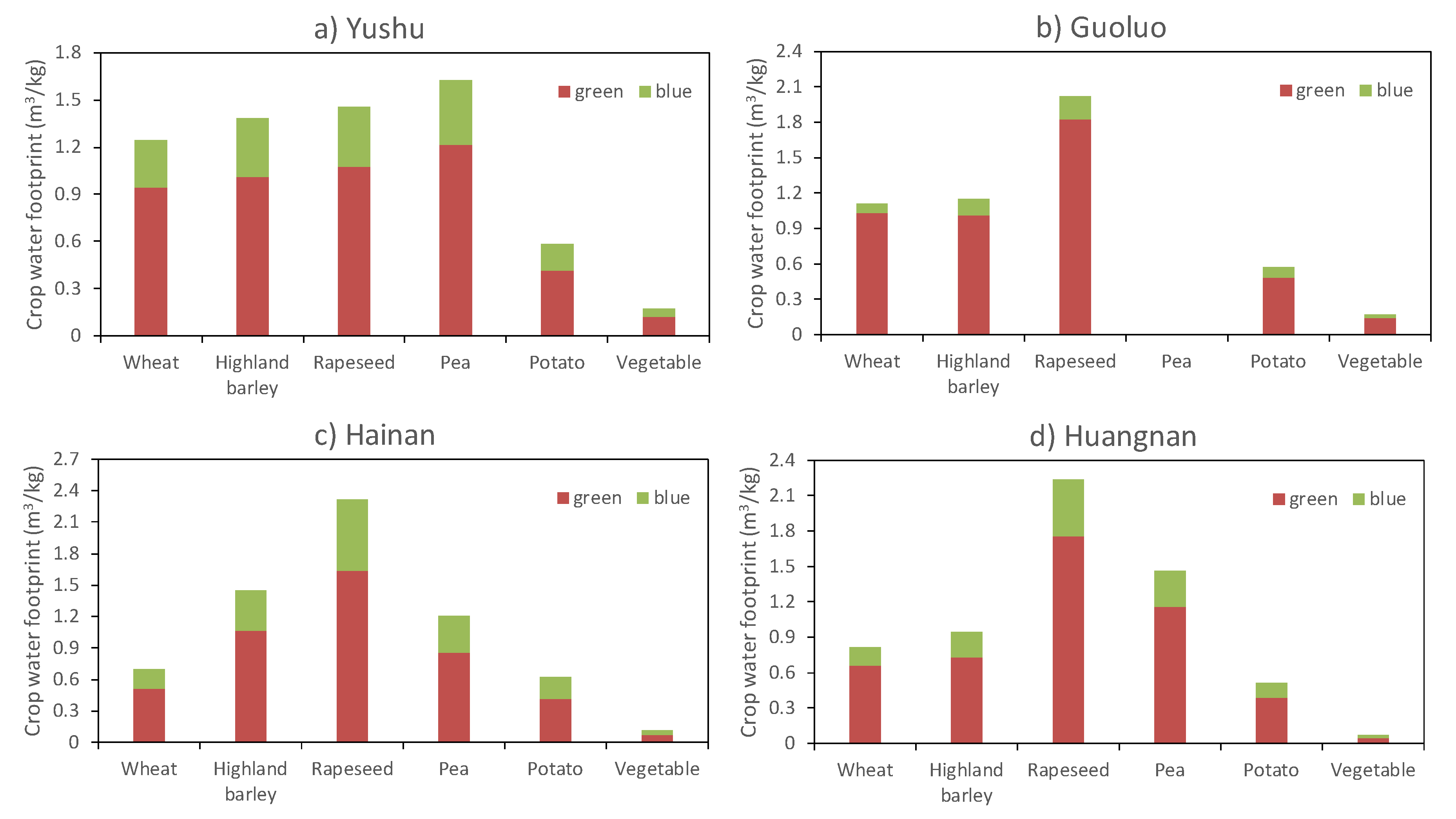
The crop evapotranspiration and crop water footprint results by regions are presented in Figure 3 and Tables S1–S4. The crop water footprint represents the blue and green water consumption and the yield per unit area. More water footprints of the crop means larger water consumption in the growth period. There are obvious differences of average water footprint per unit among six types of crops. Rapeseed, highland barley, pea and wheat have more average water footprints, 2.007 m3/kg, 1.230 m3/kg, 1.076 m3/kg and 0.968 m3/kg, respectively. Potato and vegetables have fewer average water footprints (0.574, 0.134 m3/kg). The green water of six types of crops makes up 72.28% to 81.28%. This indicates that the ratios of green water use of all six crops in the TRHR are high.
The spatial distribution of water footprint per unit mass of six crops varies in the TRHR region. For rapeseed, the water footprint is higher in Hainan and Huangnan, and lower in Yushu and Guoluo. Yushu and Huangnan show more water footprints of pea, while the values are lower in Hainan (the yield of Guoluo is very small and the water footprint could be ignored). The high-value region of the highland barley water footprint is located in Hainan and Yushu, while the low-value region in Huangnan. The water footprints of wheat water are more in Yushu and Guoluo, and fewer in Hainan. The maximum potato water footprint is in Yushu, and the minimum in Huangnan. The difference of vegetable water footprint is smaller in all four autonomous prefectures in Tibet. A comprehensive comparison of crop water footprint shows that the water footprint of all six crops in Hainan is low, indicating a high water use rate. The spatial difference of water footprint of six crops is caused by the differences of climate and soil in the four regions. Through the analysis of the spatial difference of water footprint of various crops, decisional support is provided for optimization of crop planting and efficient use of agricultural water resource.

4.2. Optimal Plans of Crop Cultivation Reconfiguration

Qinghai Province greatly depends on external grain. To reduce the dependence and ensure food security, the optimization of water footprint planting structure should be carried out on the premise of meeting local food demand first, and the planting area of crops with small water footprint with more economic benefits should be optimized. The optimization results of the crop planting area in the TRHR are shown in Table 6. Compared with the current situation of crops, wheat, rapeseed and highland barley have lower economic benefit with larger water consumption. Thus, the planting area of these crops is not added in Yushu, Guoluo and Huangnan. Due to the self-sufficiency of grain in Hainan, the area of two low-yielding and high-water-consumption crops, namely highland barley, and rapeseed, has been greatly reduced. As peas and potatoes are water crops with low water consumptions and high yields (0.802, 0.942 million yuan/hm2), the planting area in Yushu autonomous prefecture increased slightly. As vegetable has the highest yield (93.46 million yuan /hm2) and the lowest water consumption, the planting area in Yushu has increased slightly and the planting area in Guoluo has increased largely. Limited by regional water resources, Hainan produces a large amount of high water consumption grain, and the planting area of peas and vegetables has been reduced.
Based on the above optimization results of the planting area, economic benefits of 8321 million yuan, 15,737 million yuan, 51,080 million yuan and 332.02 million yuan can be gained respectively in Yushu, Guoluo, Hainan and Huanan, and the total income of the TRHR reaches 1083.4 million yuan. Due to the climatic conditions, Hainan maintains a high yield per unit area and a low water footprint of crops, so its economic benefits is much higher than those of the other three Tibetan autonomous prefectures. Due to the huge food gap in Qinghai Province, Yushu, Guoluo, Hainan and Huangnan need to shoulder the costs of 24,035 million yuan, 14,852 million yuan, 8114 million yuan and 104.12 million yuan respectively in purchasing grain, and the total cost of purchased grain in the TRHR reaches 574.13 million yuan.

4.3. Discussion

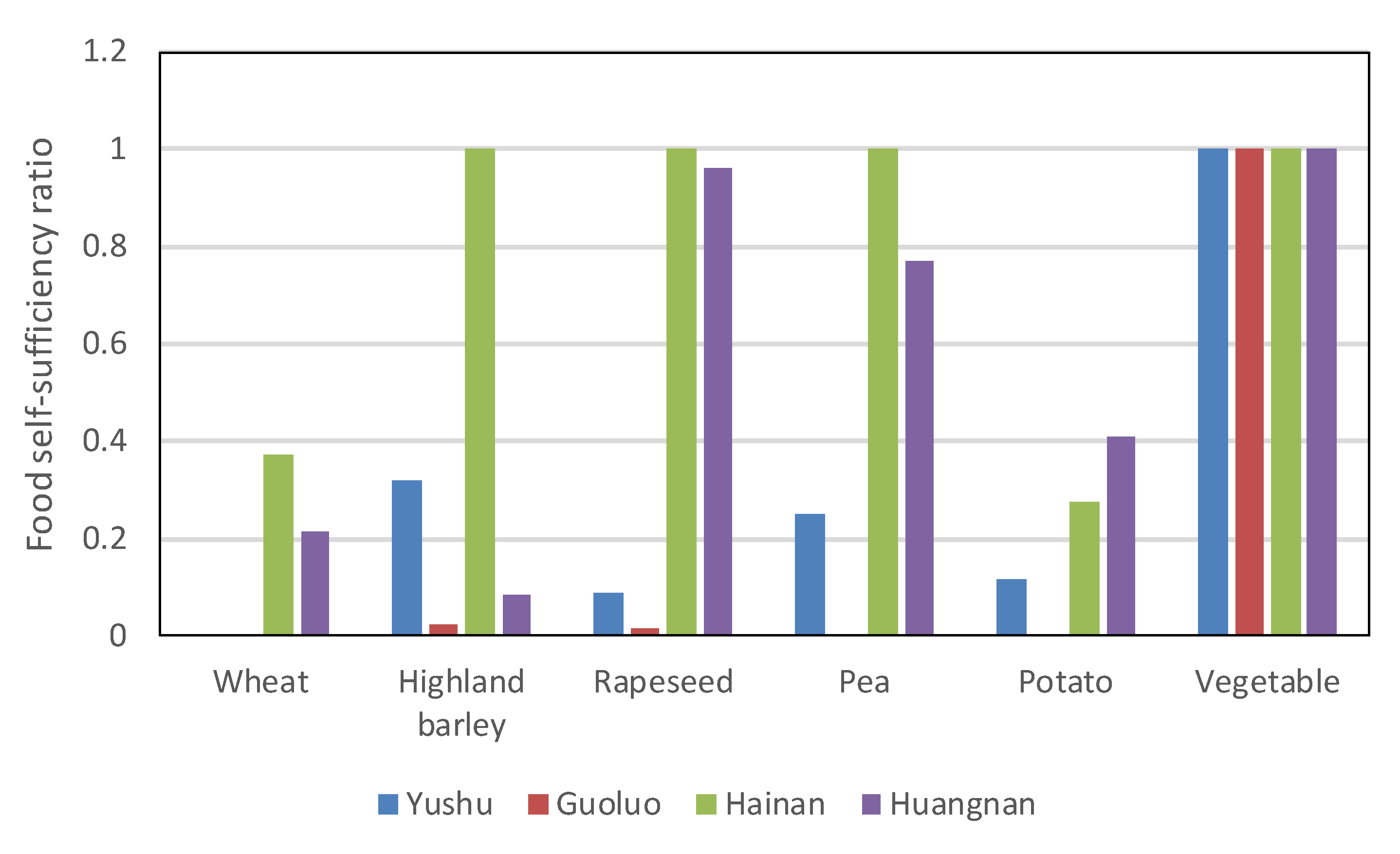
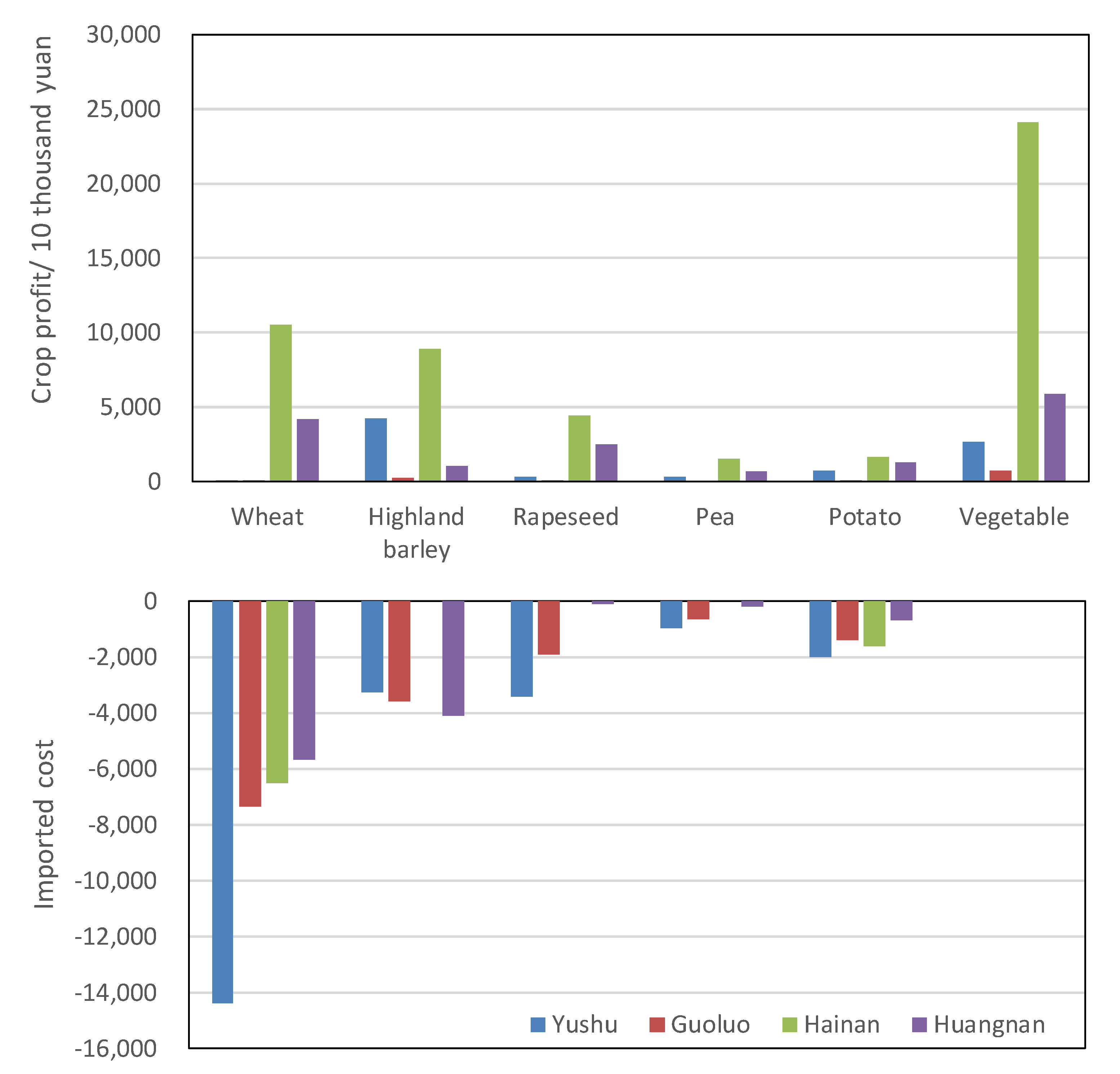
Qinghai Province mainly relies on food import, and the cereal self-sufficiency ratio reached 46% in the period 2010–2015 [59]. The same situation existed in the TRHR region. Hainan has the largest food self-sufficiency ratio, followed by Huangnan, Yushu, and Guoluo Tibetan Autonomous Prefectures (as shown in Figure 4). Based on the daily dietary guidelines for Chinese residents, oil crops (rapeseed) and pea can basically meet local demands (in Huangnan and Hainan), while the cereal shortage is huge. In Hainan Tibetan autonomous prefecture, 27%–37% of the wheat and potato is imported, while the rest of crops can meet the local demand. In Huangnan, 80% of wheat and barley are imported from other places. Wheat in Yushu and Guluo, and more than 90% of potato and barley in Guluo are dependent on import and foreign grains, leading to large import costs (as shown in Figure 5). The vegetable intake of residents in Qinghai Province was about 41 kg per capita in the period from 1984 to 2012 [60,61], which is obviously lower than the nationally recommended value [58]. Following such dietary structure, the vegetable supply of four Tibetan autonomous prefectures can reach self-sufficiency. Due to low crop water footprints and high production capacity, Hainan and Huangnan should plant more wheat, highland barley, and potato, then cereal shortage can be relieved to a certain extent.
Figure 5 presents the comparisons between crop cultivation profits and imported costs. As main intake cereals, wheat and barley are demanded much more than that of other crops. Insufficient production capacity of wheat and barley in the TRHR Region leads to high imported costs. Given special climate conditions and limited agricultural irrigation water resource, food self-sufficiency is impossible in none of the regions of the TRHR. Due to low water consumption and high selling price, only vegetables can reach net profits. The cultivated area of vegetable can be increased to improve the efficiency of agricultural water use and increase poor farmers’ incomes.
According to the optimization results with the present stage (see Table 7), the planting areas of rapeseed, peas, potatoes, and vegetables have increased slightly in Yushu. Due to water supply limitation, the planting areas of highland barley, rapeseed, peas, and vegetable in Hainan are sharply reduced. Planting area ratio of vegetable in Guoluo increases by 190%. Results demonstrate that within the scope of water supply and suitable climate conditions, the area of vegetables with the high yields and low water consumption will be greatly expanded, which remains the same tendency with latest cultivted area of Guoluo in 2018 [57,62]. It indicates the accuracy and comparability of the method.
The blue water consumption of the Three-River source crops is shown in Table 8, and the agricultural irrigation in this region consumes 79.82 million m3 of water at the present stage. According to the calculation, considering the difference of the water footprint of crops, the optimized crop planting structure can save 18.79 million m3 of irrigation water in the TRHR area. The income of planting crops in TRHR is 1,079,681 million yuan (the economic income of planting crops in Yushu, Guoluo, Hainan and Huangnan is 8250 million yuan, 593 million yuan, 82,457 million yuan and 166.68 million yuan respectively), which means the income of 3.72 million yuan for the TRHR region.
To sum up, crop planting structure adjustment based on fractional planning and the water footprint theory can save water resource by 35% and increase the yield of 2% in the TRHR. Considering the characteristics and differences of water footprint in regions planting crops, the advantages of crop planting in different regions can be brought into play to optimize the area of crops and irrigation water with high yield of water saving, so as to improve the efficiency of water resource use and effective use coefficient of farmland irrigation water and fundamentally reduce the consumption of blue water.

5. Conclusions

A land-water-food nexus framework with optimized allocation of agricultural water and land resources with food security and resource constraints is proposed in this article. The crop water footprint is combined with agricultural production restructuring to solve various constraints of water, land and food security. WFFP has been developed on sustainable land-water-food nexus management. Compared with the existing crop planning method, this model incorporates crop water footprint in the optimization process. WFFP can also tackle multiple objectives by ratio optimization, which does not lead to objectively weighing multiple objectives. Fuzziness associated with the selling price and production cost of crops is effectively tackled and incorporated into the modeling process. WFFP has been successfully applied in the TRHR, an arid irrigation area in northwest China, one of the most ecologically vulnerable areas with the most severe water shortage throughout the world. Efficient use of agricultural water resource gave priority to crop planning and management. WFFP tailored to the case study is formulated to maximize economic benefits and minimize blue water footprint in fields with physical limitations of water and land resources.
Results show that potato and vegetables have the fewest average water footprints in the TRHR, while rapeseed, highland barley, pea, and wheat have the largest average water footprints. Vegetables, peas, and potato should be the three most cultivated crops in the study area. Based on the daily dietary guidelines for Chinese residents, oil crops (rapeseed) and pea can basically meet local demands (Huangnan and Hainan), while the cereal is of a huge shortage. Considering the low crop water footprints and high production capacity of cereal, more wheat, highland and potato should be planted in Hainan and Huangnan, so as to relieve the cereal shortage to a certain extent. If vegetable intake of residents of Qinghai province in the period from 1984 to 2012 (41 kg per capita) is maintained, the vegetable supply in the four Tibetan Autonomous Prefectures can reach self-sufficiency. An optimal plan regarding crop cultivation reconfiguration with minimized crop water footprints have been generated. Compared to the status quo, the optimized plan would increase economic benefits by 2% and save water by 34%, respectively, with the limited available irrigation water.
In the future research, the impact of climate change should be considered in the land-water-food nexus. Changes in water quantity due to climate change are expected to affect crop yield which may determine food availability, stability, access and use. This may lead to damaged food security especially in arid regions. The impact of future climate change on land-water-food nexus will be further explored. Besides, energy security should be considered in the framework as the land-water-energy-food (LWEF) nexus. It can quantify interdependencies among nexus elements, push for holistic approaches that promote all nexus constituents and provide a platform for testing transformative thinking, revolutionary concepts and advancements in technology and management techniques. Such ingredients are necessary to improve overall production efficiency instead of productivities of separated sectors.

Supplementary Materials

Following materials are available online at https://www.mdpi.com/2077-0472/10/4/104/s1: Table S1, Crop evapotranspiration in Yushu Autonomous Prefecture in Tibet; Table S2, Crop evapotranspiration in Guoluo Autonomous Prefecture in Tibet; Table S3, Crop evapotranspiration in Hainan Autonomous Prefecture in Tibet; Table S4, Crop evapotranspiration in Huangnan Autonomous Prefecture in Tibet.

Author Contributions

M.C. undertook raw data collection, modelling, data analysis, as well as paper writing with the contribution of S.S. and W.L. All authors have read and agreed to the published version of the manuscript.

Funding

This research was funded by Strategic International Science and Technology Innovation Cooperation Project (grant number 2016YFE0201900).

Conflicts of Interest

The authors declare no conflict of interest.

References

  1. Kang, S.; Hao, X.; Du, T.; Tong, L.; Su, X.; Lu, H.; Li, X.; Huo, Z.; Li, S.; Ding, R. Improving agricultural water productivity to ensure food security in China under changing environment: From research to practice. Agric. Water Manag. 2017, 179, 5–17. [Google Scholar] [CrossRef]
  2. FAO. Scarcity and Degradation of Land and Water: Growing Threat to Food Security. 2011. Available online: http://www.fao.org/news/story/en/item/95153/icode/ (accessed on 1 September 2019).
  3. Misselhorn, A.; Aggarwal, P.; Ericksen, P.; Gregory, P.; Horn-Phathanothai, L.; Ingram, J.; Wiebe, K. A vision for attaining food security. Curr. Opin. Environ. Sustain. 2012, 4, 7–17. [Google Scholar] [CrossRef]
  4. Niu, G.; Zheng, Y.; Han, F.; Qin, H. The nexus of water, ecosystems and agriculture in arid areas: A multiobjective optimization study on system efficiencies. Agric. Water Manag. 2019, 223, 10569. [Google Scholar] [CrossRef]
  5. Ren, D.; Yang, Y.; Yang, Y.; Richards, K.; Zhou, X. Land-Water-Food Nexus and indications of crop adjustment for water shortage solution. Sci. Total Environ. 2018, 626, 11–21. [Google Scholar] [CrossRef]
  6. Duan, W.; Chen, Y.; Zou, S.; Nover, D. Managing the water-climate- food nexus for sustainable development in Turkmenistan. J. Clean. Prod. 2019, 220, 212–224. [Google Scholar] [CrossRef]
  7. Darshana, A.; Ostrowski, M.; Pandey, R.P. Simulation and optimization for irrigation and crop planning. Irrig. Drain. 2012, 61, 178–188. [Google Scholar] [CrossRef]
  8. Li, M.; Guo, P. A multi-objective optimal allocation model for irrigation water resources under multiple uncertainties. Appl. Math. Model. 2014, 38, 4897–4911. [Google Scholar] [CrossRef]
  9. Bas, E. A robust optimization approach to diet problem with overall glycemic load as objective function. Appl. Math. Model. 2014, 38, 4926–4940. [Google Scholar] [CrossRef]
  10. Gephart, J.A.; Davis, K.F.; Emery, K.A.; Leach, A.M.; Galloway, J.N.; Pace, M.L. The environmental cost of subsistence: optimizing diets to minimize footprints. Sci. Total Environ. 2016, 553, 120–127. [Google Scholar] [CrossRef] [Green Version]
  11. Jiang, Y.; Xu, X.; Huang, Q.; Huo, Z.; Huang, G. Optimizing regional irrigation water use by integrating a two-level optimization model and an agrohydrological model. Agric. Water Manag. 2016, 178, 76–88. [Google Scholar] [CrossRef] [Green Version]
  12. Varade, S.; Patel, J.N. Determination of Optimum Cropping Pattern Using Advanced Optimization Algorithms. J. Hydrol. Eng. 2018, 23, 05018010. [Google Scholar] [CrossRef]
  13. Garza-Díaz, L.E.; DeVincentis, A.J.; Sandoval-Solis, S.; Azizipour, M.; Ortiz-Partida, J.P.; Mahlknecht, J.; Cahn, M.; Medellin-Azuara, J.; Zaccaria, D.; Kisekka, I. Land-Use Optimization for Sustainable Agricultural Water Management in Pajaro Valley, California. J. Water Resour. Plan. Manag. 2019, 145, 05019018. [Google Scholar] [CrossRef] [Green Version]
  14. Li, M.; Singh, V.P. Sustainability of water and energy use for food production based on optimal allocation of agricultural irrigation water. Int. J. Water Resour. Dev. 2019, 36, 528–546. [Google Scholar] [CrossRef]
  15. Niu, G.; Li, Y.P.; Huang, G.H.; Liu, J.; Fan, Y.R. Crop planning and water resource allocation for sustainable development of an irrigation region in China under multiple uncertainties. Agric. Water Manag. 2016, 166, 53–69. [Google Scholar] [CrossRef]
  16. Elleuch, M.A.; Anane, M.; Euchi, J.; Frikha, A. Hybrid fuzzy multi-criteria decision making to solve the irrigation water allocation problem in the Tunisian case. Agric. Syst. 2019, 176, 102644. [Google Scholar] [CrossRef]
  17. Cheviron, B.; Vervoort, R.W.; Albasha, R.; Dairon, R.; Le Priol, C.; Mailhol, J.C. A framework to use crop models for multi-objective constrained optimization of irrigation strategies. Environ. Model. Softw. 2016, 86, 145–157. [Google Scholar] [CrossRef]
  18. PCampana, P.E.; Zhang, J.; Yao, T.; Andersson, S.; Landelius, T.; Melton, F.; Yan, J. Managing agricultural drought in Sweden using a novel spatially-explicit model from the perspective of water-food-energy nexus. J. Clean. Prod. 2018, 197, 1382–1393. [Google Scholar] [CrossRef]
  19. Habteyes, B.G.W.; Frank, A. Economics of irrigation water conservation: Dynamic optimization for consumption and investment. J. Environ. Manag. 2000, 258, 110040. [Google Scholar] [CrossRef]
  20. Mortada, S.; Najm, M.A.; Yassine, A.; El Fadel, M.; Alamiddine, I. Towards sustainable water-food nexus: An optimization approach. J. Clean. Prod. 2018, 178, 408–418. [Google Scholar] [CrossRef]
  21. YNie, Y.; Avraamidou, S.; Xiao, X.; Pistikopoulos, E.N.; Li, J.; Zeng, Y.; Song, F.; Yu, J.; Zhu, M. A Food-Energy-Water Nexus approach for land use optimization. Sci. Total Environ. 2019, 659, 7–19. [Google Scholar]
  22. Liu, X.; Guo, P.; Li, F.; Zheng, W. Optimization of planning structure in irrigated district considering water footprint under uncertainty. J. Clean. Prod. 2019, 210, 1270–1280. [Google Scholar] [CrossRef]
  23. Li, M.; Fu, Q.; Singh, V.P.; Liu, D.; Li, T.; Zhou, Y. Managing agricultural water and land resources with tradeoff between economic, environmental, and social considerations: A multi-objective non-linear optimization model under uncertainty. Agric. Syst. 2020, 178, 102685. [Google Scholar] [CrossRef]
  24. Ren, C.; Guo, P.; Tan, Q.; Zhang, L. A multi-objective fuzzy programming model for optimal use of irrigation water and land resources under uncertainty in Gansu Province, China. J. Clean. Prod. 2017, 164, 85–94. [Google Scholar] [CrossRef]
  25. Li, M.; Fu, Q.; Singh, V.P.; Ji, Y.; Liu, D.; Zhang, C.; Li, T. An optimal modelling approach for managing agricultural water-energy-food nexus under uncertainty. Sci. Total Environ. 2019, 651, 1416–1434. [Google Scholar] [CrossRef]
  26. Tang, Y.; Zhang, F.; Wang, S.; Zhang, X.; Guo, S.; Guo, P. A distributed interval nonlinear multiobjective programming approach for optimal irrigation water management in an arid area. Agric. Water Manag. 2019, 220, 13–26. [Google Scholar] [CrossRef]
  27. Linker, R.; Ioslovich, I.; Sylaios, G.; Plauborg, F.; Battilani, A. Optimal model-based deficit irrigation scheduling using AquaCrop: A simulation study with cotton, potato and tomato. Agric. Water Manag. 2016, 163, 236–243. [Google Scholar] [CrossRef]
  28. Dunnett, A.; Shirsath, P.B.; Aggarwal, P.K.; Thornton, P.; Joshi, P.K.; Pal, B.D.; Khatri-Chhetri, A.; Ghosh, J. Multi-objective land use allocation modelling for prioritizing climate-smart agricultural interventions. Ecol. Model. 2018, 381, 23–35. [Google Scholar] [CrossRef]
  29. Davijani, M.H.; Banihabib, M.E.; Anvar, A.N.; Hashemi, S.R. Multi-objective optimization model for the allocation of water resources in arid regions based on the maximization of socioeconomic efficiency. Water Resour. Manag. 2016, 30, 927–946. [Google Scholar] [CrossRef]
  30. Tan, Q.; Zhang, S.; Li, R. Optimal Use of AgriculturalWater and Land Resources through Reconfiguring Crop Planting Structure under Socioeconomic and Ecological Objectives. Water 2017, 9, 488. [Google Scholar] [CrossRef]
  31. Galan-Martin, A.; Vaskan, P.; Anton, A.; Esteller, L.J.; Guillén-Gosálbez, G. Multi-objective optimization of rainfed and irrigated agricultural areas considering production and environmental criteria: a case study of wheat production in Spain. J. Clean. Prod. 2017, 140, 816–830. [Google Scholar] [CrossRef]
  32. Li, M.; Fu, Q.; Singh, V.P.; Liu, D. An interval multi-objective programming model for irrigation water allocation under uncertainty. Agric. Water Manag. 2018, 196, 24–36. [Google Scholar] [CrossRef]
  33. Ren, C.; Li, Z.; Zhang, H. Integrated multi-objective stochastic fuzzy programming and AHP method for agricultural water and land optimization allocation under multiple uncertainties. J. Clean. Prod. 2019, 210, 12–24. [Google Scholar] [CrossRef]
  34. Lu, S.S.; Liu, Y.S.; Long, H.L.; Xing, G. Agricultural production structure optimization: a case study of major grain producing areas, China. J. Integr. Agric. 2013, 12, 184–197. [Google Scholar] [CrossRef]
  35. Fuss, S.; Havlík, P.; Szolgayova, J.; Schmid, E.; Reuter, W.H.; Khabarov, N.; Kraxner, F. Global food security & adaptation under crop yield volatility. Technol. Forecast. Soc. Chang. 2015, 98, 223–233. [Google Scholar]
  36. Hoekstra, P.Q.H. Virtual Water Trade: A Quantification of Virtual Water Flows Between Nations in Relation to International Crop Trade Value of Water Research Report Series No. 11; IHE: Delft, The Netherlands, 2002. [Google Scholar]
  37. Allan, T. Virtual Water: A Long Term Solution for Water Short Middle Eastern Economies? Occasional Paper 3, School of Oriental and African Studies (SOAS); University of London: London, UK, 1997. [Google Scholar]
  38. FAO. Food Balance Sheets, a Handout; Food and Agriculture Organization: Rome, Italy, 2001. [Google Scholar]
  39. Hoekstra, A.Y.; Chapagain, A.K.; Aldaya, M.M.; Mekonnen, M.M. The Water Footprint Assessment Manual: Setting the Global Standard; Earthscan: London, UK, 2011. [Google Scholar]
  40. FAO. CROPWAT 8.0 Model; FAO, Ed.; Food and Agriculture Organization: Rome, Italy, 2010; Available online: https://www.fao.org/nr/water/infores_databases_cropwat.html (accessed on 7 October 2019).
  41. Allen, R.G.; Pereira, L.S.; Raes, D.; Smith, M. Crop Evapotranspiration: Guidelines for Computing Crop Water Requirements; FAO: Rome, Italy, 1998. [Google Scholar]
  42. Dastane, N.G. Effective Rainfall in Irrigated Agriculture; Food and Agriculture Organization: Rome, Italy, 1978. [Google Scholar]
  43. Brouwer C, H.M. Irrigation Water Management: irrigation Water Needs; Training Manual No. 3; FAO: Rome, Italy, 1986. [Google Scholar]
  44. Hess, T. Estimating green water footprints in a temperate environment. Water 2010, 2, 351–362. [Google Scholar] [CrossRef]
  45. SCS, U. Irrigation water requirements. United States Department of Agriculture, soil conservation service. Tech. Rel. 1970, 21, 88. [Google Scholar]
  46. Smith, M. CROPWAT—A Computer Program for Irrigation Planning and Management; FAO: Rome, Italy, 1992. [Google Scholar]
  47. Charnes, A.; Cooper, W.W. Programming with linear fractional functionals. Nav. Res. Logist. Quart. 1962, 9, 181–186. [Google Scholar] [CrossRef]
  48. Zadeh, L.A. Fuzzy sets as a basis for a theory of possibility. Fuzzy Sets Syst. 1978, 1, 3–28. [Google Scholar] [CrossRef]
  49. Tanaka, H.; Guo, P.; Zimmermann, H.J. Possibility distributions of fuzzy decision variables obained from possibilisitc linear programming problems. Fuzzy Sets Syst. 2000, 113, 323–332. [Google Scholar] [CrossRef]
  50. Watada, N.A.a.J. Fractile optimization approach for possibilistic programming problem. In Proceedings of the International Conference on Man-Machine System (ICoMMS’ 12), Malaysia, 27–28 February 2012. [Google Scholar]
  51. Prade, D.D.a.H. Possibility Theory: An Approach to Computerized Processing of Uncertainty; Plenum Press: New York, NY, USA, 1988. [Google Scholar]
  52. Zhou, Y.; Li, Y.P.; Huang, G.H.; Huang, Y. Development of Optimal Water-Resources Management Strategies for Kaidu-Kongque Watershed under Multiple Uncertainties. Math. Probl. Eng. 2013, 2013, 892321. [Google Scholar] [CrossRef]
  53. Bureau of Statictics of Yushu Tibetan Autonomous Prefecture. National Economy and Society Developed Statistical Bulletin of Yushu Tibetan Autonomous Prefecture in 2015–2017. 2018. [Google Scholar]
  54. Bureau of Statictics of Huangnan Tibetan Autonomous Prefecture. National Economy and Society Development Statistical Bulletin of Huangnan Tibetan Autonomous Prefecture in 2015–2017. 2018. [Google Scholar]
  55. Bureau of Statictics of Hainan Tibetan Autonomous Prefecture. National Economy and Society Development Statistical Bulletin of Hainan Tibetan Autonomous Prefecture in 2015–2017. 2018. [Google Scholar]
  56. Bureau of Statictics of Guoluo Tibetan Autonomous Prefecture. National Economy and Society Development Statistical Bulletin of Guoluo Tibetan Autonomous Prefecture in 2015–2017. 2018. [Google Scholar]
  57. Statistics Bureau of Qinghai Municipality. Qinghai Statistical Yearbook in 2018; Statistics Bureau of Qinghai Municipality China Statistical Press: Qinghai, China, 2018.
  58. Society, T.C.N. Dietary Guidelines for Chinese Resident: Beijing. 2016. [Google Scholar]
  59. CNR. cn. Qinghai Actively Promoted the Adjustment of Industrial Structure to Achieve the Rapid Economic Development. 2019. Available online: https://www.sohu.com/a/122036531_115496 (accessed on 10 February 2020). (In Chinese).
  60. Hong, Z. The study the changes of diets strucutre among Qinghai inhabitants living in urban and rural areas (in Chinese). J. Qinghai Med Coll. 2003, 24, 159–161. [Google Scholar]
  61. Hong, Z. Dietary structure change analysis about urban and rural residents from 1985 to 2012 in Qinghai province (in Chinese). Henan J. Prev. Med. 2015, 26, 1–4. [Google Scholar]
  62. Bureau of Statictics of Guoluo Tibetan Autonomous Prefecture. National Economy and Society Development Statistical Bulletin of Guoluo Tibetan Autonomous Prefecture of 2019. 2019. Available online: http://tjj.qinghai.gov.cn/tjData/cityBulletin/201903/t20190327_60279.html (accessed on 10 February 2020).
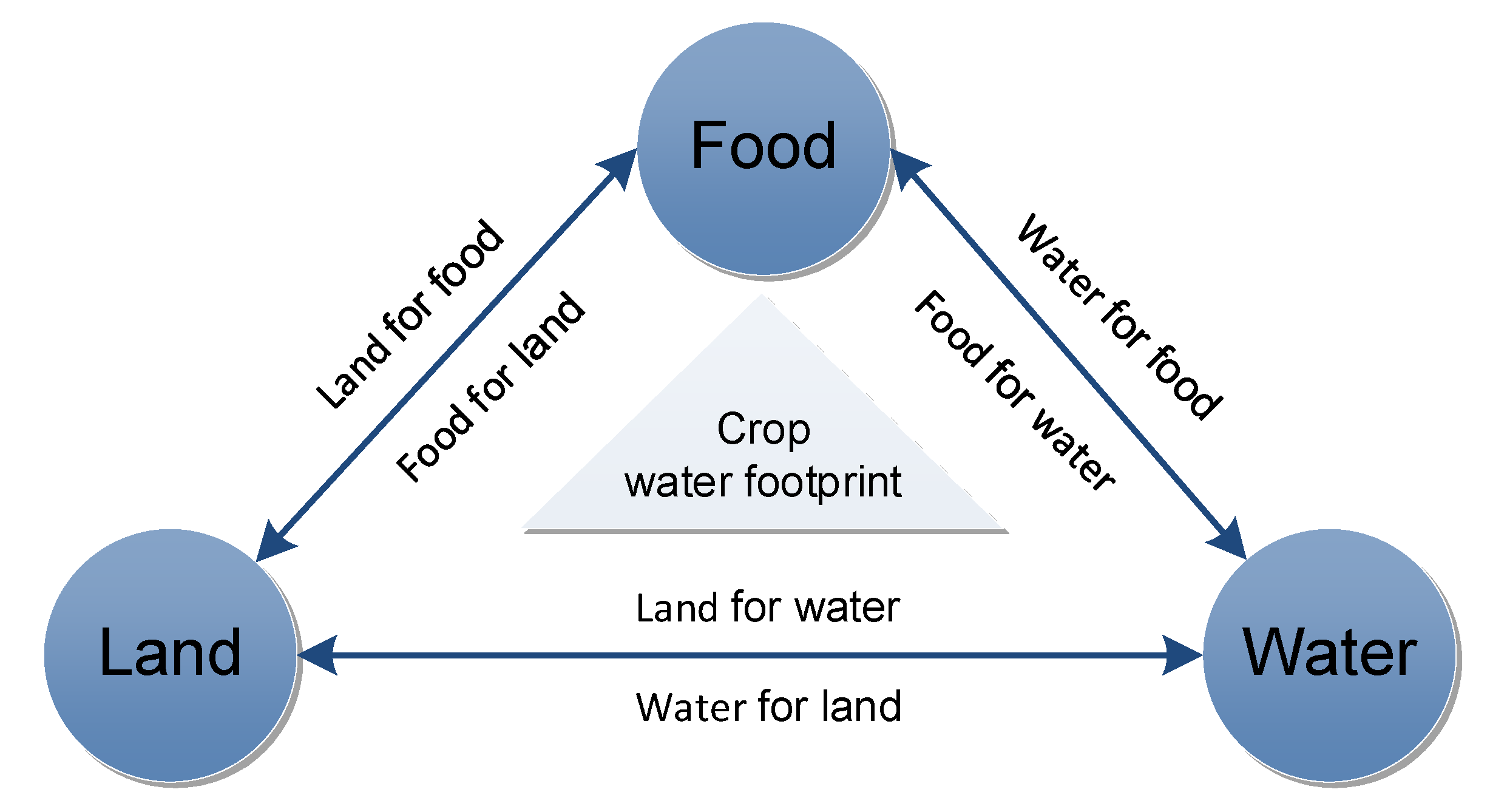
Figure 1. Land-water-food nexus framework.
Agriculture 10 00104 g001
Figure 2. Crop coefficient of the TRHR. 4-1, 4-2, and 4-3 respectively show the first, middle and last ten days of April; 5-1, 5-2, and 5-3 respectively show the first, middle and last ten days of May; 6-1, 6-2, and 6-3 respectively show the first, middle and last ten days of June; 7-1, 7-2, and 7-3 respectively show the first, middle and last ten days of July; 8-1, 8-2, and 8-3 respectively show the first, middle and last ten days of August.
Agriculture 10 00104 g002
Figure 3. Crop water footprints of the TRHR. (a)—(d) respectively refer to Yushu, Guoluo, Hainan, and Huangnan Tibetan autonomous prefectures.
Agriculture 10 00104 g003
Figure 4. Food self-sufficient ratios of the TRHR.
Agriculture 10 00104 g004
Figure 5. Comparisons of cultivation profits and imported crop costs.
Agriculture 10 00104 g005
Table 1. Daily Meteorological data of the TRHR.
MonthPrecipitation (mm)Daily Minimum Temperature (°C)Daily Maximum Temperature (°C)Relative HumidityWind Speed (m/s)Sunshine Duration
Yushu16.50−17.35−1.335.011.487.06
20.50−13.543.423.422.006.72
37.35−7.098.363.452.287.05
426.48−3.429.365.312.197.18
560.250.6413.395.892.047.13
697.685.1016.916.681.816.34
738.483.8018.485.811.899.03
863.984.8718.736.151.746.89
991.004.7018.016.881.706.95
108.60−3.9812.055.191.657.75
111.33−9.568.263.921.527.09
120.33−14.841.093.721.466.08
Guoluo18.38−19.35−1.015.14 1.75 7.28
20.98−15.303.183.71 2.39 7.07
313.06−9.187.374.41 2.36 6.67
428.20−5.258.425.51 2.23 7.24
559.60−0.7612.456.07 2.24 7.11
6124.784.2515.366.96 1.96 5.95
764.202.7416.256.60 1.77 8.46
867.083.4316.526.69 1.94 6.94
9110.023.7415.067.29 1.84 5.62
1018.80−4.1310.965.75 1.82 7.70
113.76−9.856.954.89 1.87 7.12
122.82−17.48−1.194.98 1.64 6.71
Hainan11.00−17.472.033.37 1.76 7.41
20.00−14.324.712.75 2.56 7.89
30.00−9.239.452.76 2.49 7.72
428.80−3.3211.414.31 2.33 8.19
552.500.4414.595.37 2.55 7.23
671.405.0816.786.38 1.94 6.01
757.404.6718.466.44 1.90 8.48
849.004.1019.296.39 1.95 7.82
947.303.3515.186.96 1.63 4.72
108.00−5.8112.674.66 1.90 8.26
113.50−11.207.834.39 2.05 7.94
120.00−20.14−0.923.48 1.73 7.53
Huangnan113.00−22.190.175.44 1.11 7.33
22.50−16.464.333.81 2.35 7.77
38.30−9.948.054.56 2.16 7.42
421.00−5.009.525.36 2.30 8.40
560.80−0.4513.056.40 2.46 7.51
6107.304.2515.266.93 2.37 5.98
738.502.1116.657.00 2.06 8.58
871.702.3017.067.25 1.94 7.98
965.303.3813.977.63 2.32 4.83
1024.60−4.8311.706.42 2.03 7.41
119.40−11.437.455.71 1.71 7.49
124.90−20.85−0.585.06 1.57 7.15
Table 2. Crop prices and crop production costs in Qinghai Province.
Price/(yuan·kg−1)Production Cost/(yuan·hm−2)
Wheat(2.10, 2.30, 2.50)(46.89, 48.89, 50.89)
Highland barley(2.20, 2.40, 2.60)(6.17, 6.67, 7.17)
Rapeseed(3.80, 4.20, 4.60)(42.05, 45.05, 48.05)
Pea(5.5, 6.0, 6.5)(10.67, 12.67, 14.67)
Potato(2.60, 2.80, 3.00)(76.07, 80.07, 84.07)
Vegetable(4.69, 5.19, 5.69)(222.48, 227.48, 232.48)
Table 3. Crop area in the TRHR (hm2).
YushuGuoluoHainanHuangnan
Wheat675010,2364758
Highland barley757339743,8401317
Rapeseed3734520,2674347
Pea26701253528
Potato6271215261194
Vegetable333333200347
Table 4. Per unit yield in the TRHR (kg/hm2).
YushuGuoluoHainanHuangnan
Wheat2591278944843849
Highland barley2340273421001906
Rapeseed2326147813081357
Pea1965025842146
Potato4182422838674651
Vegetable15,00015,03022,68727,500
Table 5. Water resource situations in the TRHR (104 m3).
Total Water SupplyIrrigation Water UseTotal Water ConsumptionIrrigation Water ConsumptionTotal Water Consumption
Yushu356726135671753064
Guoluo20011472001981670
Hainan31,61322,77930,73115,05920,670
Huangnan52942997525519513712
Table 6. Optimized plant area in the TRHR (hm2) (pnes = 0.8).
YushuGuoluoHainanHuangnan
Wheat675010,2364758
Highland barley757339719,7731317
Rapeseed3774580954347
Pea2730983528
Potato6321215261008
Vegetable340962051301
Table 7. Change ratios of optimized plant area (%) (pnes = 0.8).
YushuGuoluoHainanHuangnan
Wheat0000
Highland barley00−54.90
Rapeseed1.10−60.10
Pea2.20−21.60
Potato0.800−15.6
Vegetable2.1190−35.9−13.3
Table 8. Optimized blue water amount in the TRHR (104 m3) (pnes =0.8).
YushuGuoluoHainanHuangnan
Wheat5.11.1881.3291.1
Highland barley666.314.31425.495.8
Rapeseed30.91.3716.6281.4
Pea22.2090.934.5
Potato44.40.4121.062.3
Vegetable29.14.2186.1345.7
Sum798.121.33421.3110.9