Article

Multiresponse Optimization of Cutting Force and Cutting Power in Chopping Agricultural Residues Using Grey-Based Taguchi Method

1
Administration Office, Thai Nguyen University, 3/2 Street, Tichluong Ward, Thainguyen City 251750, Vietnam
2
Information and Library Center, Thai Nguyen University of Technology, 3/2 Street, Tichluong Ward, Thainguyen City 251750, Vietnam
3
Faculty of International Training, Thai Nguyen University of Technology, 3/2 Street, Tichluong Ward, Thainguyen City 251750, Vietnam
4
Faculty of Mechanical Engineering, Thai Nguyen University of Technology, 3/2 street, Tichluong Ward, Thainguyen City 251750, Vietnam
*
Author to whom correspondence should be addressed.
Agriculture 2020, 10(3), 51; https://doi.org/10.3390/agriculture10030051
Submission received: 29 January 2020 / Revised: 21 February 2020 / Accepted: 24 February 2020 / Published: 25 February 2020
(This article belongs to the Section Crop Production)

Abstract

:
Agricultural residues are the most abundant biomass and forage resources. Chopping is a precondition for either use, and reducing the shearing force has been considered as one of the most effective way to save energy. A smaller force can also permit more compact mechanical parts of chopping devices. In several cases, power consumption may be large, even when the shearing force is small, if the corresponding cutting velocity is high. Consequently, it is important to minimize both cutting force and power consumption simultaneously. This paper presents a practical approach to solve the multi-objective optimization problem for chopping processes of corn stalks. Applying the Taguchi design of experiments, a plan of 27 chopping tests was conducted. Based on the grey relational grade analysis and analysis of variance technique, optimum levels as well as the percentage contribution of such parameters were identified. Experimental results showed that the multi-response optimization problem in chopping corn stalks can be effectively addressed through the combination of Taguchi design and grey relational analysis. The results can be expanded for practical applications in design and operation of chopping machines for agricultural residues.

1. Introduction

Agricultural residues are the most important resources for biomass and animal feeding. Size reduction is an important prerequisite to produce forage and biomass energy. Nevertheless, this procedure was also considered as one of the most energy-inefficient tasks [1,2]. The efficiency of the size reduction has typically been assessed through the amount of cutting force and energy required [3,4,5]. It has been found that equipment using shear mode for size reduction may hold promise for improved energy efficiency [6]. The energy required for cutting forage stems has been evaluated for a wide range of plant species, cutting velocities, moisture contents, and stem sizes [7]. The results were classified into three categories [8]: quasistatic shearing (cutting velocities less than 30 mm/s), cutting with a counter-edge (at velocities greater than 0.5 m/s), and impact cutting without a counter-edge (at speeds up to 60 m/s). It has been shown that minimal energy is required for quasistatic shearing and for cutting with a counter-edge. Prasad and Gupta [9] found specific energies for corn stalks in the range of 19–24 mJ/mm2 in quasistatic measurements. However, the energies required for impact cutting are generally 1 or 2 orders of magnitude greater than those recorded for quasistatic or counter-edge cutting [8].
Quasistatic tests have been used in many studies of cutting force and cutting energy for various kinds of agricultural residues. For example, the change of shear force and energy of cotton stalk were evaluated by Pekitkan and Eliçin [10]. Another quasistatic test using a universal machine was implemented to study the effects of diameter and age of grape canes on cutting force and energy [11]. Using the same experimental apparatus, the effects of moisture content, internode region, and oblique angle on the mechanical properties of sainfoin stem were evaluated by Boydaş et al. [12]. Other authors [13] found that the shearing angle has a strong effect on the cutting force and specific energy. A smaller cutting angle was related to a larger cutting resistance.
Impact cutting tests have been investigated in many studies, where the effect of various factors on the force and energy were evaluated. For corn stalks, Prasad and Gupta [9] showed that the optimum values of bevel angle, knife approach angle, and shear angle providing the minimum cutting force and energy consumption were 23°, 32°, and 55°, respectively. An investigation by Azadbakht and Zahedi [4] showed that the effects of height, moisture content, and their interaction on cutting energy are significant. The energy consumption during impact cutting of canola stalk [14] was considered as a function of moisture content and cutting height.
Generally, agricultural chopping systems are designed based on two main cutting principles: scissor shearing to provide shear stress, and rotary knives to generate both impact and shear stress on the stalks [15]. For the first case, the plants to be cut are pressed against the fixed counter edge with the help of cutter. The knife speed is resolved into two components: chopping speed, which penetrates into the material, and the sliding cut speed [16].
The analysis of the literature above indicates that cutting speed and blade geometry have strong effects on cutting force and cutting energy for agricultural residues. Most of the investigations had been done for impact cutting with a single knife. Several others have functioned with counter edge cutting but under quasistatic mode, where the cutting velocity is extremely low. There have been few studies on chopping processes with counter edges and under high-velocity conditions. Besides, it is worth noting that the power consumption may be large, even when the shearing force is small, if the corresponding cutting velocity is high. Consequently, it is expected to minimize both cutting force and power consumption simultaneously. A recent investigation with such purpose was conducted using factorial experimental designs [17]. The main aims of this study are to provide another approach of solving such problem by using Taguchi–grey relational analysis technique. The Taguchi method with grey relational analysis (GRA) has been employed in several experimental investigations in agriculture and biotechnology [18,19,20,21]. However, there has not been found a similar study for optimization of chopping agricultural residues.

2. Materials and Methods

2.1. Experimental Setup

The setup was made based on the outline of a 93ZP-1000 straw chopper produced by the Liaoning Fengcheng Donfeng Machinery Factory (Liaoning, Dandong, China). Figure 1 illustrates a 3D model of the chopping device.
In Figure 1, a belt wheel (1) receives and transfers drive torque from a Direct-current (DC) motor to the cutting knifes (3) via the main spindle (2). Being made in the form of a circular sector, the cutter can be easily adjusted to obtain a required approach angle α by using the screw (4) and the clamp set (5). In the figure, the position of the stalk to be cut (6) is determined by two angles: the feed angle β and the tilt angle φ. In this study, the tilt angle φ remained at 90°.
The experimental setup was then implemented as illustrated in Figure 2. In this figure, all parts are labelled similar to those in Figure 1. As mentioned, the approach angle α is adjusted by the screw (4) and the clamp set (5) (Figure 2a). In addition, a dynamic force sensor (9) is used to measure instant cutting force. In Figure 2b, the way to adjust the feed angle β by the clamp set (10) is illustrated.
The force sensor model 9712A500 (Kistler, Winterthur, Switzerland), with sensitivity of 2.4729 mV/N, was placed under the counter shear bar to measure the cutting force. A DAQ model NI-USB-6008 (National Instruments, Austin, Texas, USA) and the Ni Signal Express software were employed to collect the cutting force data. The experimental rig was driven by a commercial 1.5 kW DC motor, working with a voltage supply ranging from 50 to 220 V. By adjusting the voltage provided by an Alternating-current (AC) variable transformer combined with a rectifier, the variable speed of the cutting spindle could be obtained. The maize stalks used for this experimental study were kept in an air-conditioned room for one week after harvest from the fields in the northern part of Vietnam. The wet basis moisture content of the samples was then measured by drying–weighting method. The wet basis moisture content was around 81%.

2.2. The Multiobjective Function

The average power consumption is the amount of energy consumed per unit time. Consequently, given a cutting force Fc and the corresponding cutting velocity V, the cutting power Pc can be expressed as:
P c = F c × V
In chopping machines, where a number of knifes are equally arranged on a rotating disk, the cutting force signal appears as a train of periodic, near identical pulses, as shown in Figure 3a. The peaks of the cutting force signal were collected for this experimental study.
With the chopping disk driven by an electrical motor, it can be assumed that the cutting velocity is approximately constant during each cutting process. Applying Equation (1), the instantaneous cutting power at a function of time can be obtained from the cutting force signal, as shown in Figure 3b.
Denoting the period as T, i.e., the time between two consecutive chopping processes, the energy consumed for cutting during such time can be expressed as:
E p u l s e = 0 T p ( t ) d t
The total consumed power then can be calculated by:
P = 1 T 0 T p ( t ) d t = E p u l s e T
denoting the pulse time as τ so that:
E p u l s e = P p e a k × τ
The duty cycle of the pulse train then can be defined as:
P P p e a k = τ T
In this study, the duration of each cutting pulse is approximately calculated as the time required for a point on the cutting edge to completely pass the stalk diameter. To simplify the calculation, the stalk diameters are assumed to be their average value and thus a constant, assigned as daverage. In this study, daverage was set to be 0.02 m. Consequently, the pulse time τ is defined as:
τ = d a v e r a g e V
Finally, the power consumption at a certain cutting velocity V can be calculated as:
P = τ T P p e a k = d a v e r a g e V . T F p e a k . V = 1 T d a v e r a g e . F p e a k
To simplify the notation in the experimental analysis, the peak value of the cutting force in each chopping event will be considered as demonstrative of cutting force and thus will be noted as the cutting force F in this study. Consequently, the multiobjective optimisation problem can be expressed as:
min ( F ( α , β , V ) , P ( α , β , V ) )

2.3. Design of Experiments and Multiobjective Optimization Process

In this study, the approach angle, the feed angle and the cutting velocity were selected to be three experimental variables. The design of experiments was built using three parameters at three levels each, leading to the L27(33) orthogonal array of tests. The investigated parameters and their levels considered in this study are shown in Table 1.
As mentioned, the two objective responses, including peak values of cutting force and cutting power, were selected for the optimization process. Once the normalized signal-to-noise (S/N) ratio values of the responses were calculated, corresponding grey relational coefficients were carried out. The grey relational analysis was then implemented in order to find the trade-off optimum condition. Detailed steps of calculation techniques and results are presented in the next section.

3. Results and Discussions

3.1. Step 1: Calculate the S/N Ratios

Firstly, the S/N ratio for the corresponding responses was calculated. Since minimization of all outputs is intended, the following formula for the case of smaller-the-better was employed:
S / N ( η ) = 10 l o g 10 ( 1 n i = 1 n y i j 2 )
where n is number of replications, yij is observed response value, I = 1, 2,…, n; j = 1, 2,…, k.
Table 2 shows the input factor values and output responses of all 27 tests which were planned by the Taguchi design, where each set of inputs was replicated three times, and the corresponding S/N ratios calculated using the Equation (9). The cutting force was measured by the force sensor. The cutting power was calculated using Equation (7).

3.2. Step 2: Calculate Normalized S/N Ratios and Grey Relational Coefficients

In order to formulate the data for the grey relation analysis, S/N ratios were then normalized. An appropriate value is deducted from the values in the same array to make the value approximate to 1. The normalized S/N ratios were calculated for S/N ratio with smaller-the-better manner, using the following expression:
Z i j = m a x ( y i j , i = 1 , 2 , n ) y i j m a x ( y i j , i = 1 , 2 , n ) m i n ( y i j , i = 1 , 2 , n )
The normalized S/N ratio values obtained were then used to calculate the grey relational coefficients by using the following formula:
γ ( y 0 ( k ) , y i ( k ) ) = Δ m i n + ξ Δ m a x Δ 0 j ( k ) + ξ Δ m a x
where j = 1, 2,…, n; k = 1, 2,…, m; n is the number of experimental data items and m is the number of responses; y0(k) is the reference sequence; yi(k) is the specific comparison sequence; Δ0j is the absolute value of the difference between y0(k) and yj(k); Δmin and Δmax are the smallest and largest values of yi(k), respectively; ξ is the distinguishing coefficient, 0 ≤ ξ ≤ 1.
The normalized S/N ratio values and the corresponding grey relational coefficients are given in Table 3.

3.3. Step 3: Perform Analysis of Variance (ANOVA)

Analysis of variance (ANOVA) was performed to identify the effect of individual factors. The percentage of contribution calculated from ANOVA can be used to estimate the importance of each parameter on the performance responses. The results of ANOVA and contribution of each factor are depicted in the Table 4.
As can be seen from Table 4, the approach angle has the most significant effect on the responses (58%), followed by the feed angle (22%) and then the spindle speed (7%).

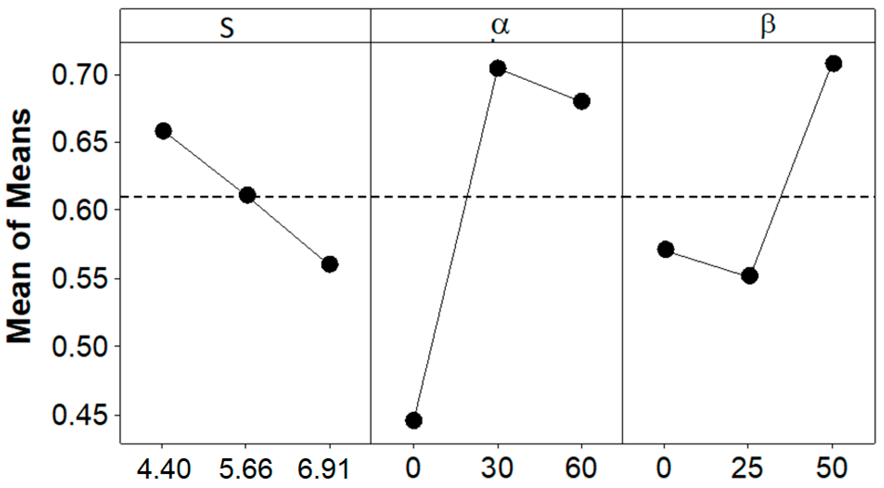
3.4. Step 4: Calculate Grey Relational Grades and Determine the Optimum Cutting Condition

Next, the grey relational grades were calculated using the following formula:
γ j ¯ = 1 k i = 1 m γ i j
Table 5 shows the grey relational grades with respect to the different levels of input parameters. Since the higher grey relational grade indicates a better product quality, the optimal level for each input parameter was determined as the highest value in the investigated range. Such values were underlined in Table 5. The data were then plotted Figure 4.
In conclusion, the optimum parameters for minimizing both cutting force and cutting power were determined as follows: the velocity was at level 1, i.e., 4.40 m/s; the approach angle was at level 2, i.e., at 30°, and the feeding angle was at level 3, i.e., at 50°. Doing validation tests with the above optimum inputs, a cutting force of 251.7 N and cutting power of 26.2 W were obtained. Looking back at the 27 tests run before, as shown in Table 2, there were two tests (number 9 and number 15) that would be considered as providing either the smallest force or smallest power. For comparison purpose, the inputs and response values of these two tests and the optimum set are represented in Table 6.
As can be seen in Table 6, the test number 9 provided the smallest cutting power, compared to other 26 tests, with P = 26.32 W. However, the cutting force at that condition was of 263.6 N, higher than that of other tests. Similarly, the test number 15 gave the smallest cutting force as 242.6 N but with a high cutting power of 36.39 W. The optimum input (shown in the last row of the table) provided a combination of both relatively small cutting force (251.7 N) and cutting power (26.2 W).

4. Conclusions

In chopping of agricultural residues, the cutting force can decrease at higher velocity, but high velocity would also lead to increased power consumption. The optimum parameters of this multiresponse problem in chopping corn stalks can be determined by employing Taguchi experimental design combined with grey relational analysis. The cutting force and cutting power thus can both reach the smallest values.

Author Contributions

Conceptualization, V.-D.V., K.-T.H. and V.-D.N.; Data curation, T.-T.N., N.-H.C. and Q.-H.N.; Formal analysis, T.-T.N., N.-H.C. and K.-T.H.; Investigation, V.-D.V.; Methodology, N.-H.C. and V.-D.N.; Resources, T.-T.N.; Software, Q.-H.N.; Supervision, V.-D.N. All authors have read and agreed to the published version of the manuscript.

Funding

This research received no external funding.

Acknowledgments

The authors would like to express their thanks to Thai Nguyen University and TNU University of Technology (Thai Nguyen University of Technology) for all supports and encouragements.

Conflicts of Interest

The authors declare no conflict of interest.

References

  1. Mohsenin, N.N. Physical Properties of Plant and Animal Materials: Structure, Physical Characteristics, and Mechanical Properties; Gordon and Breach: London, UK, 1986. [Google Scholar]
  2. Bitra, V.S.; Womac, A.; Igathinathane, C.; Miu, P.I.; Yang, Y.T.; Smith, D.R.; Chevanan, N.; Sokhansanj, S.; Cannayen, I. Direct measures of mechanical energy for knife mill size reduction of switchgrass, wheat straw, and corn stover. Bioresour. Technol. 2009, 100, 6578–6585. [Google Scholar] [CrossRef] [PubMed]
  3. Igathinathane, C.; Pordesimo, L.; Schilling, M.; Columbus, E. Fast and simple measurement of cutting energy requirement of plant stalk and prediction model development. Ind. Crop. Prod. 2011, 33, 518–523. [Google Scholar] [CrossRef]
  4. Azadbakht, M.; Asl, A.R.; Zahedi, K.T. Energy Requirement for Cutting Corn Stalks. Int. J. Biol. Biomol. Agric. Food Biotechnol. Eng. 2014, 8, 479–482. [Google Scholar]
  5. Allameh, A.; Alizadeh, M.R. Specific cutting energy variations under different rice stem cultivars and blade parameters. Idesia 2016, 34, 11–17. [Google Scholar] [CrossRef]
  6. Igathinathane, C.; Womac, A.; Sokhansanj, S.; Cannayen, I. Corn stalk orientation effect on mechanical cutting. Biosyst. Eng. 2010, 107, 97–106. [Google Scholar] [CrossRef]
  7. O’Dogherty, M. A review of research on forage chopping. J. Agric. Eng. Res. 1982, 27, 267–289. [Google Scholar] [CrossRef]
  8. McRandal, D.; McNulty, P. Impact cutting behaviour of forage crops I. Mathematical models and laboratory tests. J. Agric. Eng. Res. 1978, 23, 313–328. [Google Scholar] [CrossRef]
  9. Prasad, J.; Gupta, C. Mechanical properties of maize stalk as related to harvesting. J. Agric. Eng. Res. 1975, 20, 79–87. [Google Scholar] [CrossRef]
  10. Pekitkan, F.G.; Eliçin, A.K. The Change of Shear Force and Energy of Cotton Stalk. Agronomy 2018, 61, 360–366. [Google Scholar]
  11. Esgici, R.; Pekitkan, F.G.; Ozdemir, G. Cutting Parameters of Some Grape Varieties Subject to the Diameter and Age of Canes. Fresenius Environ. Bull. 2019, 28, 167–170. [Google Scholar]
  12. Boydaş, M.G.; Çomakli, M.; Sayinci, B.; Kara, M. Effects of moisture content, internode region, and oblique angle on the mechanical properties of sainfoin stem. Turk. J. Agric. For. 2019, 43, 254–263. [Google Scholar] [CrossRef] [Green Version]
  13. Igathinathane, C.; Womac, A.; Sokhansanj, S.; Narayan, S.; Cannayen, I. Size reduction of high- and low-moisture corn stalks by linear knife grid system. Biomass Bioenergy 2009, 33, 547–557. [Google Scholar] [CrossRef]
  14. Azadbakht, M.; Esmaeilzadeh, E.; Esmaeili-Shayan, M. Energy consumption during impact cutting of canola stalk as a function of moisture content and cutting height. J. Saudi Soc. Agric. Sci. 2015, 14, 147–152. [Google Scholar] [CrossRef] [Green Version]
  15. Ghahrae, O.; Khoshtaghaza, M.; Ahmad, D.B. Design and development of special cutting system for sweet sorghum harvester. J. Cent. Eur. Agric. 2008, 9, 469–474. [Google Scholar]
  16. Bernacki, H.; Haman, J.; Kanafojski, C. Agricultural Machines, Theory and Construction; NTIS: Springfield, VA, USA, 1972.
  17. Vu, V.-D.; Ngo, Q.-H.; Nguyen, T.-T.; Nguyen, H.-C.; Nguyen, Q.-T.; Nguyen, V.-D. Multi-objective optimisation of cutting force and cutting power in chopping agricultural residues. Biosyst. Eng. 2020, 191, 107–115. [Google Scholar] [CrossRef]
  18. Nor Mohamed, S.A.; Zainudin, E.S.; Sapuan, S.M.; Md. Deros, M.A.; Arifin, A.M.T. Integration of Taguchi-Grey Relational Analysis Technique in Parameter Process Optimization for Rice Husk Composite. BioResJournal 2019, 14, 1110–1126. [Google Scholar]
  19. Musabbikhah, H.S.; Subarmono, M.; Wibisono, A. Modelling and Optimization of the Best Parameters of Rice Husk Drying and Carbonization by Using Taguchi Method with Multi Response Signal to Noise Procedure. Int. J. Renew. Energy Res. 2017, 7, 1219–1227. [Google Scholar]
  20. Shyam Thapa, M.A.M.; Humphrey, K.; Engelken, R. Optimization of process parameters in the pelletization of crop residues by taguchi-grey relational analysis. Int. J. Agric. Environ. Biores. 2018, 3, 60–74. [Google Scholar]
  21. Deepanraj, B.; Sivasubramanian, V.; Jayaraj, S. Multi-response optimization of process parameters in biogas production from food waste using Taguchi—Grey relational analysis. Energy Convers. Manag. 2017, 141, 429–438. [Google Scholar] [CrossRef]
Figure 1. A 3D model of the experimental setup. (1) belt wheel; (2) spindle shaft; (3) knife; (4) screw; (5) clamp; (6) maize stalk; (7) counter shear; (8) torque sensor.
Agriculture 10 00051 g001
Figure 2. Practical experimental setup: (a) a front view (the protection cover was opened) and (b) a side view: (3) knife; (4) screw; (5) clamp; (6) maize stalk; (7) counter shear; (8) torque sensor; (9) force sensor and (10) clamp set.
Agriculture 10 00051 g002
Figure 3. Example of experimental cutting force and power consumption signals.
Agriculture 10 00051 g003
Figure 4. Factor effects on grade values.
Agriculture 10 00051 g004
Table 1. Experimental parameters and their levels
ParametersInput Parameter Levels
Level 1Level 2Level 3
Velocity (m/s), V4.405.666.91
Approach angle (°), α03060
Feeding angle (°), β02550
Table 2. The L27 orthogonal array, experimental results and corresponding signal-to-noise (S/N) ratios.
#Input FactorsResponsesS/N Ratios
V (m/s)α (°)β (°)Force (N)Power (W)ForcePower
14.4000706.0782.3748−56.977−38.316
24.4000617.6872.0627−55.815−37.154
34.4000502.1058.5788−54.016−35.355
44.403025313.9936.6322−49.938−31.277
54.403025264.1330.8152−48.436−29.775
64.403025276.6032.2700−48.837−30.176
74.406050261.9430.5597−48.364−29.703
84.406050269.8031.4767−48.621−29.960
94.406050263.6026.3200−48.419−28.406
105.66025485.1072.7650−53.717−37.238
115.66025479.4471.9160−53.615−37.137
125.66025414.8462.2260−52.358−35.879
135.663050312.8646.9290−49.907−33.429
145.663050255.0738.2605−48.133−31.655
155.663050242.6036.3900−47.698−31.220
165.66600287.9343.1895−49.186−32.708
175.66600267.5340.1295−48.547−32.069
185.66600261.8739.2805−48.362−31.884
196.91050344.5963.1748−50.746−36.011
206.91050317.3958.1882−50.032−35.297
216.91050289.0652.9943−49.220−34.485
226.91300307.1956.3182−49.748−35.013
236.91300273.2050.0867−48.730−33.994
246.91300250.5345.9305−47.977−33.242
256.916025385.3870.6530−51.718−36.983
266.916025361.5966.2915−51.164−36.429
276.916025317.3958.1882−50.032−35.297
Table 3. Normalized values of S/N ratios and grey relational coefficients.
#Normalized Values of S/N RatiosGrey Relational CoefficientsGrey GradeOrder
10.0000.0000.3330.3330.33327
20.1250.1170.3640.3620.36326
30.3190.2990.4230.4160.42023
40.7580.7100.6740.6330.65411
50.9200.8620.8630.7830.8233
60.8770.8210.8030.7370.7706
70.9280.8690.8740.7920.8332
80.9000.8430.8340.7610.7985
90.9221.0000.8651.0000.9331
100.3510.1090.4350.3590.39725
110.3620.1190.4390.3620.40124
120.4980.2460.4990.3990.44922
130.7620.4930.6770.4970.58715
140.9530.6720.9140.6040.7597
151.0000.7161.0000.6380.8194
160.8400.5660.7570.5350.64612
170.9080.6300.8450.5750.71010
180.9280.6490.8750.5880.7318
190.6710.2330.6030.3940.49919
200.7480.3050.6650.4180.54217
210.8360.3870.7530.4490.60114
220.7790.3330.6930.4290.56116
230.8890.4360.8180.4700.64413
240.9700.5120.9430.5060.7259
250.5670.1340.5360.3660.45121
260.6260.1900.5720.3820.47720
270.7480.3050.6650.4180.54218
Table 4. Analysis of variance for means.
SourceDegree of FreedomSeq SSAdj SSAdj MSF ValueP ValueContribution (%)
V20.014500.014500.0072510.460.6837
α20.123270.123270.0616353.940.20358
β20.043700.043700.0218501.400.41721
Residual Error20.031300.031300.015652
Total80.21278
Table 5. Corresponding grey relational grades of the tests.
LevelVαβ
10.65840.44490.5703
20.61100.70450.5514
30.56010.68010.7078
Delta0.09830.25960.1563
Rank312
Table 6. The optimum test compared to two normal tests.
Test No.V (m/s)α (°)β (°)F (N)P (W)
94.406050263.6026.3200
155.663050242.6036.3900
Optimum4.43050251.726.2

