Article

STL-ATTLSTM: Vegetable Price Forecasting Using STL and Attention Mechanism-Based LSTM

1
Department of Computer Science and Engineering, Sejong University, Seoul 05006, Korea
2
Department of Bioresources Engineering, Sejong University, Seoul 05006, Korea
3
Supply & Demand Management Office, Integrated Information System Team, Korea Agro-Fisheries & Food Trade Corporation, Naju 58326, Korea
*
Author to whom correspondence should be addressed.
Agriculture 2020, 10(12), 612; https://doi.org/10.3390/agriculture10120612
Submission received: 2 November 2020 / Revised: 4 December 2020 / Accepted: 5 December 2020 / Published: 8 December 2020

Abstract

:
It is difficult to forecast vegetable prices because they are affected by numerous factors, such as weather and crop production, and the time-series data have strong non-linear and non-stationary characteristics. To address these issues, we propose the STL-ATTLSTM (STL-Attention-based LSTM) model, which integrates the seasonal trend decomposition using the Loess (STL) preprocessing method and attention mechanism based on long short-term memory (LSTM). The proposed STL-ATTLSTM forecasts monthly vegetable prices using various types of information, such as vegetable prices, weather information of the main production areas, and market trading volumes. The STL method decomposes time-series vegetable price data into trend, seasonality, and remainder components. It uses the remainder component by removing the trend and seasonality components. In the model training process, attention weights are assigned to all input variables; thus, the model’s prediction performance is improved by focusing on the variables that affect the prediction results. The proposed STL-ATTLSTM was applied to five crops, namely cabbage, radish, onion, hot pepper, and garlic, and its performance was compared to three benchmark models (i.e., LSTM, attention LSTM, and STL-LSTM). The performance results show that the LSTM model combined with the STL method (STL-LSTM) achieved a 12% higher prediction accuracy than the attention LSTM model that did not use the STL method and solved the prediction lag arising from high seasonality. The attention LSTM model improved the prediction accuracy by approximately 4% to 5% compared to the LSTM model. The STL-ATTLSTM model achieved the best performance, with an average root mean square error (RMSE) of 380, and an average mean absolute percentage error (MAPE) of 7%.

1. Introduction

Agricultural products account for a large proportion of the market as a necessity for daily consumption, and their prices play a critical part in consumer spending and agricultural household income (Statistics FAO, 2018) [1]. Agricultural product prices are determined by the supply and demand for the relevant year [2]. An oversupply of agricultural products causes vegetable prices to plummet, resulting in financial losses to agricultural households, whereas an undersupply of agricultural products increases prices, putting a burden on consumers. The imbalance of the supply and demand of agricultural products affects both farmers and consumers, and therefore, it is difficult for the government to make decisions that balance these factors [3]. The Ministry of Agriculture, Food and Rural Affairs (MAFRA), a governmental agency in South Korea, has been making efforts to stabilize producer incomes and consumer prices by designating cabbage, radishes, onion, garlic, and hot peppers as the “five major supply-and-demand-sensitive vegetables.” Nonetheless, it is not easy to control the supply and demand of agricultural products. Providing more accurate agricultural product predictions can help establish a well-planned management strategy in advance, reduce risk, and ultimately contribute to stability of supply and demand in the agricultural market [4].
In previous research on the supply and demand predictions of Korean vegetables, the Korea Rural Economic Institute (KREI) provided users with the cultivation area, unit yield, and prices in a monthly report format using the Korean Agriculture Simulation Model (KASMO). However, as the KASMO applies a single model to all 45 items of vegetables studied, it has the limitation of not accurately reflecting the characteristics of each item [5]. For example, cabbage is composed of various cropping types, such as spring cabbage, autumn cabbage, and high land cabbage (Rural Development Administration), and as the growing conditions, cultivation cycle, and main production areas of each cropping type are all different, these factors should be reflected in any model that aims to forecast vegetable prices accurately.
As the “five major supply-and-demand-sensitive vegetables” are mainly grown in open fields, production is greatly affected by climate [4,5,6]. Climate change has a direct impact on agriculture, as the weather is essential information for growing crops [7]. In particular, more accurate production prediction will be possible using weather information about the main production areas where crops are grown [8].
Therefore, in this study, we propose an STL-Attention-based LSTM (STL-ATTLSTM) model using the Loess (STL) preprocessing method and attention mechanism based on long short-term memory (LSTM); this model combines various types of information, such as vegetable prices, weather information of the main production areas, and market trading volumes to forecast vegetable prices.
This paper is organized as follows. In Section 2, a related work and the contributions of this paper are introduced. Section 3 presents a brief description of STL, LSTM, attention mechanism, and the proposed method in detail. Section 4 and Section 5 illustrate the experimental design and discuss the result, respectively. Concluding remarks are finally made in Section 6.

2. Related Work

Time-series prediction has been used in many practical applications, such as financial forecasting and agricultural price forecasting [3,9,10,11]. Traditional statistical and deep learning methods are commonly used for this forecasting. In this section, we investigate technology trends and shortcomings through studies on traditional vegetable price forecasting.

2.1. Agricultural Price Forecasting Using Statistical Methods

Various regression methods are used as traditional statistical methods. Models such as the autoregressive integrated moving average (ARIMA), generalized ARIMA, and seasonal ARIMA are typical. Assis and Remali [12] compared the prediction performance of various time-series methods for cocoa bean price forecasting; the experimental results showed that the generalized ARIMA model achieved the best performance. Adanacioglu and Yercan [13] forecast tomato prices in Turkey using seasonal ARIMA. They removed the high seasonality of tomatoes using a seasonal index. Ge and Wu [6] forecast corn prices using a multivariate linear regression model. In this study, the main effect of the supply–demand relationship was applied to the model, but the performance was still to a certain extent general in terms of the corn price changes. BV and Dakshayini [14] forecast tomato prices and demand using Holt Winter’s model and compared its performance with the benchmark models, simple linear regression and multiple linear regression. Their results showed large variations between the forecast values and real values, and Holt Winter’s model that considers seasonality showed the best performance. Apart from these studies, Darekar and Reddy [15], Jadhav et al. [16], and Pardhi et al. [17] forecast agricultural prices using the ARIMA model.
Studies on agricultural price forecasting using statistical methods can handle general linear problems but have the disadvantage that the performance is not stable for non-linear price series.

2.2. Agricultural Price Forecasting Using Machine Learning and Deep Learning Methods

Machine learning and deep learning-based algorithms are new approaches to solving time-series prediction problems. These approaches have been found to produce more accurate results than traditional regression-based models [18,19]. In recent years, with the increase in agricultural prices’ volatility, powerful learning models have been used to forecast prices.
Minghua [18] forecast time-series price data of agricultural products using a back-propagation neural network and demonstrated the superiority of the proposed artificial neural network (ANN) model by comparing it with a statistical model. Wang et al. [20] forecast garlic prices with non-linear properties using a hybrid ARIMA support vector machine (SVM) model. The performance results showed that the proposed hybrid model achieved higher prediction accuracy than single ARIMA and SVM. Nasira and Hemageetha [21] forecast weekly and monthly tomato prices using the back-propagation neural network (BPNN) algorithm. Hemageetha and Nasira [22] forecast tomato prices using a radial basis function (RBF) neural network and proved the superiority of the proposed model by comparing its performance with the BPNN model. Li et al. [23] forecast weekly egg prices in China using a chaotic neural network and compared it to the ARIMA model. The results showed that the chaotic neural network achieved a higher non-linear fitting ability and better performance than ARIMA.
In addition, hybrid models that integrate methods, such as time-series preprocessing and optimization, are often used in research on agricultural price forecasting instead of using a single model. Luo et al. [24] forecast Beijing Lentinus edodes mushroom prices by proposing four models: BPNN, RBF neural network, neural network based on genetic algorithm (GA), and an integrated model. The performance results showed that the performance of the BPNN was the lowest, the performance of the neural network (NN) based on the GA model was higher than that of the RBF neural network, and the integrated model achieved the best performance. Zhang et al. [25] forecast soybean prices in China by proposing a quantile regression-based RBF (QR-RBF) neural network model. In addition, to optimize the model, the performance was improved by applying a gradient descent with genetic algorithm (GDGA). This finding was also in agreement with previous studies [26,27]. Subhasree and Priya [28] forecast five crop prices in the Chinese market using a BPNN, RBF neural network, and GA based neural network and found that the GA-based neural network achieved the highest performance.
Xiong et al., [3] proposed a seasonal trend decomposition using Loess (STL) -based extreme learning machine method and forecast cabbage, hot pepper, cucumber, kidney bean, and tomato prices in China. This study preprocessed time-series data using the STL method by considering the seasonal characteristics of various vegetables, and as a result, it successfully forecasts vegetable prices with high seasonality. Li et al. [29] forecast vegetable prices using a model that combined a Hodrick–Prescott (H-P) filter and a neural network. The study improved forecasting accuracy by decomposing trend and cyclical components in time-series data and recombining forecast values using the H-P filter. In a previous study, Jin et al. [30] forecast five monthly crop prices in the Korean market using the STL-LSTM (long short-term memory) model. This study proved that forecasting performance was improved by eliminating high seasonality in vegetable prices. Liu et al., [31] divided hog price data into trend and cyclical components, forecast them using the most similar sub-series search method, and recombined them. Then, they forecast the hog prices using a support vector regression (SVR) prediction model. The SVR algorithm can be used for non-linear time-series prediction and works well for small datasets [32,33]. Yoo [4] forecast Korean cabbage prices using the vector autoregressive method and the Bayesian structural time-series model. Climate factors and production were used, along with trends and seasonality of price data, and the importance of meteorological data was raised because the Korean cabbage is a crop grown in open fields. Chen et al. [34] forecast cabbage prices in the Chinese market by proposing a wavelet analysis-based LSTM model. Here, the wavelet method achieved higher forecasting accuracy than the single LSTM by removing noise from time-series data.
Most studies on vegetable price forecasting using machine learning or deep learning algorithms use ANN and LSTM as their prediction models. However, for these models, an equal contribution is assigned to all input variables in the training process. An attention mechanism [35] has emerged to address this issue. The attention mechanism can calculate the importance of input variables by assigning higher weights to important input variables in the learning process. Recently, the attention mechanism has shown good performance in various fields, such as image classification, machine translation, and multimedia recommendation, and has begun to be applied to time-series data analysis.
Qin et al. [10] applied a dual-stage attention-based recurrent neural network model to stock market data, which is time-series data. They efficiently predicted prices using feature attention and temporal attention, and it became possible to explain the correlations between input variables and results. Zhang et al. [36] efficiently addressed a long-term dependence issue by automatically selecting important input variables through financial time-series prediction using an attention-based LSTM model. Ran et al., [37] performed travel-time prediction using an attention mechanism-based LSTM. The attention-based LSTM model proposed through various experiments achieved better performance than other baseline models, and the attention mechanism could focus well on the differences of input features. Li et al. [11] proposed an evolutionary attention-based LSTM model and applied it to Beijing particulate matter 2.5 (ug/m3) data. The study could resolve the relationship between local features in time-steps.
Table 1 shows the models, plant types, input variable types, processing type (seasonal or trend), and whether to use a feature engineering method, which has been proposed in traditional studies on agricultural price forecasting.

2.3. Summary and Contribution

Studies on time-series prediction using conventional statistical methods show that the volatility and periodicity of time-series data can be effectively captured and explained. However, generally, statistical methods have the disadvantage of being unable to analyze the non-stationary and non-linear relationships of time-series data [36] or to handle numerous input variables. Machine learning and deep learning algorithms generally have the advantage of handling non-stationary and non-linear data well. When analyzing studies that applied conventional machine learning or deep learning, it can be seen that these algorithms achieved better performance than the conventional statistical methods in time-series prediction. In addition, when analyzing vegetable prices with high volatility, seasonality, and trend characteristics, preprocessing processes, such as filters and STL, are known to play a crucial role compared to using raw data directly, and they have recently appeared in time-series analyses. The contributions of this study are as follows: (1) vegetable prices are affected by many factors such as weather and import/export volume, but 15 out of 21 studies mainly used the price as an input variable. In this study, we used not only price but also incorporated weather, trading volume, and import/export data. (2) Previous studies used several prediction models, such as ARIMA, seasonal ARIMA, ANN, and SVR, but only two studies used LSTM, which achieved excellent performance in time-series prediction. In this study, we used the LSTM model to forecast vegetable prices. (3) Most of the studies were applied to the Chinese and Indian markets. Of these, the number of studies conducted on the Chinese market, 11, was the largest. In this study, we verified the performance of the proposed model by applying it to five crops: cabbage, radish, onion, hot pepper, and garlic, in the South Korean market. (4) Vegetable price data includes seasonality and trend components. However, only 8 of 21 previous studies covered seasonality or trend components. In this study, we dealt with the seasonality and trend of price data using the STL method. Further, we solved the prediction lag caused by a model that did not learn well owing to high volatility and proved the importance of the STL method by comparing its performance to a model without STL. (5) The importance of the input variables used in the prediction model differs. However, only two previous studies calculated the importance of input variables and applied them to the prediction model. In this study, the importance of each input variable is calculated using the attention mechanism, and vegetable prices are forecast based on this importance. The attention mechanism has recently begun to be used for time-series prediction, but it has not been used in any research on agricultural price forecasting.

3. Methods

3.1. Time-Series Data Decomposition Using STL

STL is a time-series decomposition method that aims to decompose time-series data Y t into trend ( T t ), seasonal ( S t ), and remainder components ( R t ), which is expressed as Y t =   T t +   S t + R t . The STL algorithm consists of an outer loop and an inner loop. In the outer loop, robustness weights are assigned to each data point according to the remainder, reducing the influence of outliers. In the inner loop, the trend and seasonal components are updated, and the process is as follows.
Step 1: Detrend. By removing the calculated trend component from the inner loop, Y t   T t ( k ) is obtained. Here, k is the loop number.
Step 2: Cycle-subseries smoothing. The value of removing the trend component is broken into a cycle subseries. Each cycle subseries obtains the preliminary seasonal component S ˜ t ( k + 1 )   through the LOESS smoother.
Step 3: Low-pass filtering of the smoothed cycle subseries. Any remaining trend T ˜ t ( k + 1 ) is identified by applying a low-pass filter to S ˜ t ( k + 1 ) , obtained in Step 2.
Step 4: Detrending the smoothed cycle subseries. The seasonal component from the (k + 1) loop is: S t ( k + 1 ) =   S ˜ t ( k + 1 )   T ˜ t ( k + 1 )
Step 5: De-seasonalizing. Y t   S t ( k + 1 )
Step 6: Trend smoothing. The trend component T t ( k + 1 ) is obtained by applying the LOESS smoother to the value obtained by removing the seasonality in Step 5.
STL has several advantages. First, the STL method has the advantage of being able to handle all types of seasonality, unlike the seasonal extraction in ARIMA time series (SEAT) [38] and X11 [39] methods. Second, although the seasonal component changes over time, the user can control the change rate. Third, as outliers do not greatly impact the decomposed trend and seasonal components, it is safe to use when there are outliers.

3.2. LSTM Model

Long short-term memory (LSTM) is a special type of recurrent neural network (RNN). RNNs have been successfully applied in various fields, such as speech recognition, language modeling, machine translation, image captioning, and text recognition. One of the advantages of RNN is that it can use previous step information to solve current step problems [40]. However, with an increase in the gap between the two types of information as the predicted sequence becomes longer, RNN has a long-term dependency problem that makes it difficult to connect contexts [41]. LSTM was proposed by Hochreiter et al. [42] to solve the long-term dependency and vanishing gradient problems. LSTM has an input gate, forget gate, output gate, and cell state that are interactive in a single neural network layer. The structure of LSTM is shown in Figure 1. The forget gate performs the operation shown in Equation (1). It receives the hidden state h t 1   ( hidden   state   of   previous   time   step ) of the previous step and the input x t (input of current time-step) of the current step, and then performs matrix multiplication with the weight W f   ( learnable   forget   gate   weights ) of the forget gate. Next, after adding bias value bf (learnable forget gate bias), result f t   ( output   of   forget   gate ) is obtained through the sigmoid function. Because the sigmoid function ultimately produces a value between 0 and 1, the closer the calculated f t   value is to 1, the more information is stored in C t 1   ( cell   state   of   previous   time   step ,   C   means   cell   state ) and the closer it is to 0, the more information is discarded in C t 1 .
f t =   σ ( W f · [ h t 1 ,   x t ] +   b f )
The input gate performs the operations shown in Equation (2) and Equation (3) to determine the new information to be stored in the cell state. This process consists of two parts. In Equation (2), the first part, W i is the weight of the input gate; b i is the bias of the input gate, and these two values determine which value to update. In Equation (2), matrix multiplication is performed by multiplying   h t 1 and x t by weight Wi; bias b i   is added, and then i t (output of input gate) is obtained through the sigmoid function for the added value. Equation (3), the second part, produces a candidate vector C ˜ t that is added to the cell state. Matrix multiplication is performed by multiplying   h t 1 and x t by weight W i ; bias b C   is added, and then C ˜ t is obtained through the tanh function for the added value. The cell state of the previous time-step, C t 1 , is updated through the calculated i t and C ˜ t . The method of updating the cell state is as in Equation (4), the part to forget is forgotten by multiplying f t (output of forget gate), calculated in the forget gate, by the cell state of the previous step C t 1 and then adding the new candidate i t   × C ˜ t . The dimensions of all variables in the Equation (t) are R h , where the superscripts ℎ refer to the number of hidden units in LSTM.
i t =   σ ( W i   ×   [ h t 1 ,   x t ]   +   b i )
C ˜ t = tanh ( W C   ×   [ h t 1 ,   x t ] +   b C )
C t =   f t   × C t 1 +   i t   × C ˜ t
Finally, the output gate determines the output. The calculation of the output gate is performed as in Equations (5) and (6). As seen in Equation (5), matrix multiplication is performed by multiplying [ h t 1 ,   x t ] by the weight W o   ( learnable   output   gate   weights ) of the output gate, and the bias b o (learnable output gate bias) of the output gate is added. Then o t is obtained through the sigmoid function for the added value. For cell state C t , the tanh function is used to assign the cell state a value in [−1, 1]. This value and the o t obtained in Equation (5) are used to obtain the hidden state of the next time-step, ht, as shown in Equation (6).
o t =   σ ( W o [ h t 1 ,   x t ]   +   b o )
h t =   o t   × tanh ( C t )

3.3. Attention Mechanism

The attention mechanism was introduced in the sequence-to-sequence model for machine translation. The basic idea of the attention mechanism is to refer to the entire input sentence once more in the encoder each time the output word is predicted in the decoder. However, instead of referring to the entire input sentence at the same weight, it focuses more on the words that are related to the words to be predicted at that time. In this study, the attention layer was implemented by inspiration from the attention mechanism used in the seq2seq model. The operations performed in the attention layer are shown in Equations (7) and (8). First, matrix multiplication is performed by multiplying the three-dimensional input X by the weight W a and adding bias b a . Here, the dimensions of the input X refer to the batch size (number of samples to be applied for attention mechanism), time-step, and feature number. The input shape of W a is set to (feature_num, feature_num) to obtain the same number of outputs as the feature number, which is the third dimension of the input X; thus, W a X +   b a can be considered an attention score. Next, attention weight A w is obtained through the softmax function for the attention score. A w is three-dimensional data with a shape (batch size, time-step, feature number) and has a probability distribution where the sum of each feature number dimension is 1. The average is calculated based on the time-step dimension, which is the second dimension of A w , and then data with a shape (batch size, 1, feature number) is obtained. Next, to make the shapes of all input X the same, the data of A w is repeated as many times as the number of time-steps based on the second dimension, and an A ¯ w   is obtained that has the same shape as A w . The final attention weight A ¯ w obtained in this way is multiplied by input X, as shown in Equation (8), to obtain the weighted result   A o .
A w = softmax ( W a X +   b a )
A o =   A ¯ w × X
A o , the result of applying the attention weight obtained through the learning of W a and b a for each input variable, was used as an input to the LSTM model. To identify the importance of each feature before inputting it to the LSTM model using this method, a dot-product attention operation was added to calculate the attention weight. By adding the attention layer, it is possible to identify which input variable has a significant impact on model prediction through the weight of each input variable.

3.4. Proposed STL-ATTLSTM Method

The STL-ATTLSTM model proposed in this study is composed of data preprocessing, price prediction, and output; its structure is shown in Figure 2.
In the data preprocessing step, vegetable price data is decomposed into the seasonality, trend, and remainder components using the STL method. Of these, the derived variables of price are created in the remainder component. Next, input variables are learned through the attention layer, and attention weights are assigned to all input variables. The input variables assigned with attention weights are learned through the LSTM model, and the vegetable prices for the next month are forecast. In the output, the forecast vegetable prices for the next month and the attention weights trained in the attention layer are output.
The structure and hyperparameters of the attention and LSTM models used in this study are shown in Table 2. The proposed model is composed of attention, LSTM, and fully connected layers. In the attention layer, the weight for input variables is output through the softmax activation function. The number of cell units of the LSTM layer connected behind the attention layer was set to six, and tanh was used as the activation function. To avoid the overfitting issue, a dropout layer was added, and the rate was set to 0.2. The proposed model used two fully connected layers. The number of neurons is set to 10 in the first layer and 1 in the second layer. Finally, the vegetable prices are output in the node.
The model was trained for 1000 epochs and retrain with the best epoch. The best epoch is the epoch with the lowest verification loss. We used the Adam optimizer with a learning rate of 0.001, beta_1 = 0.9, beta_2 = 0.999.

4. Research Design

This section describes the data used and the performance evaluation criteria and presents the experimental method for measuring the performance of the proposed model. We conducted two experiments in this study. In the first experiment, we determined the optimal time-step value for the proposed STL-ATTLSTM model. In the second experiment, we compared the performance of the proposed STL-ATTLSTM to three benchmark models, LSTM, attention LSTM, and STL-LSTM.

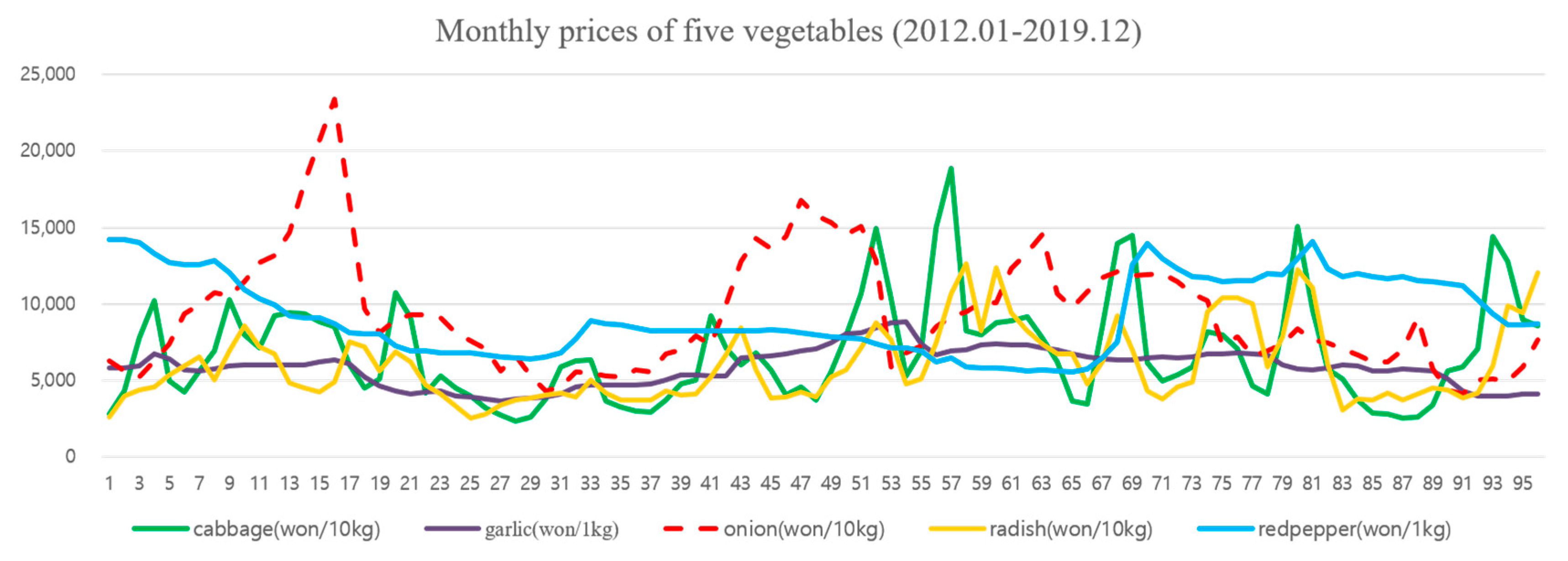
4.1. Dataset Description

In this study, we forecast monthly prices of five crops, cabbage, radishes, onion, hot peppers, and garlic, using vegetable prices, weather information about the main production areas, and import/export data of vegetables from January 2012 to December 2019. The price trend of each crop is shown in Figure 3. The data collected from January 2012 to June 2019 were used as training data, and the data from July 2019 to December 2019 were used as test data.
Vegetable price data were downloaded from the Outlook and Agricultural Statistics Information System (KREI OASIS) [43] and Korea Agricultural Marketing Information Service (aT KAMIS) [44]. As the vegetable price data are daily data, we grouped them on a monthly basis and used the average values as our monthly data.
Vegetable prices are closely related to the relevant year’s agricultural production. However, because production statistics are released after the year ends, it is difficult to use production data directly for monthly forecasting. To address this issue, we used the trading volume in the vegetable market. The trading volume refers to the volume that vegetables are brought into the market; it can replace production data in a sense. The trading volume data is provided daily by Outlook & Agricultural Statistics Information System (KREI OASIS) [43]. We also grouped the trading volume data on a monthly basis and used the accumulated values.
The meteorological data used in this study were collected in the Korean Meteorological Administration (KMA) [45]. The weather information we used comprises the average temperature, average minimum temperature, average humidity, cumulative precipitation, minimum temperature days, maximum temperature days, typhoon advisories, and typhoon warnings in the main production areas. The day of a typhoon advisory and typhoon warning was indicated as 1, and the cumulative value grouped by month was used. As the main production areas of vegetables can change from year to year, we designed the model with these factors. We selected the three main production areas for each vegetable crop type and used weather information about the harvest time instead of the entire cultivation time. For example, the cultivation time for highland cabbages is usually from March to September, but in this study, we used the meteorological information from three main production areas from July to September, which was the harvest time. Table 3 shows a summary of the harvest times and main production areas of cabbage and radish by crop type. Here, the cultivation time for vegetables by crop type was provided by aT, and the cultivation area data by crop type was collected from the Korean Statistical Information Service (KOSIS) [46]. In this study, we used meteorological data only for the prediction of cabbage and radish prices, not for the other crops. The reason behind this is that cabbage and radish are brought into the market immediately after they have been harvested in the field. When it rains during the harvest period, they are dried in warehouses for two or three days and then brought back to the market. Conversely, as hot pepper, onion, and garlic are not immediately brought into the market and instead are stored in warehouses, they are expected to be less affected by the weather at harvest time.
Vegetable prices are also closely related to import/export volumes. With an increase in the import volume, vegetable prices decrease. In recent times, because of various reasons, the cultivation area has been decreasing, and the volume of cheap imported vegetables has been increasing. Therefore, we used import/export volume information in this study. Import/export data are provided monthly from Korea Agro-fisheries & Food Trade Corporation (aT NongNet) [47], and are applied to the cabbage, radish, and onion prices.
Table 4 shows the descriptions and formulas of the input variables used in this study, price variables, incoming volume variables, meteorological variables, and other variables. To prevent prediction lag in time-series data prediction, we generated all variables except the current price using the remainder component value.

4.2. Measurement Criteria

In this study, we used two performance indices to measure the prediction performance of the model, root mean square error (RMSE), and mean absolute percentage error (MAPE).
RMSE is an index that measures the difference between the real value and the predicted value, and it is expressed as shown in Equation (9). To obtain the RMSE, the predicted value is first subtracted from the real value of each data sample. Then, the squared value is added, and the added value is divided by the number of samples. Next, the square root of the result is obtained. Here, y ^ t in Equation (9) refers to the predicted value for the number of data samples t, and y t refers to the real value for the data sample t. The RMSE value is always non-negative, and the closer to 0, the fewer the errors.
RMSE =   t = 1 T ( y ^ t y t ) 2 T
MAPE is an index used to measure the accuracy of a prediction model in statistics, and it is expressed as shown in Equation (10).
MAPE =   1 n t = 1 n | A t   F t A t |
In Equation (10), A t refers to an actual measured value, and F t refers to a predicted value. To obtain MAPE, the difference between A t and F t is calculated and then divided by A t . Next, the absolute values of the divided values are summed, and then the summed value is divided by the number of samples to obtain the average. A percentage error can be calculated by multiplying this value by 100%. MAPE is relatively intuitive compared to RMSE because the error rate is expressed as a percentage regardless of domain knowledge.

4.3. Optimal Time-Step Search

LSTM is an algorithm that handles time-series data, and the user must set a time-step value that determines how much data comprises every single instance. It is a highly crucial hyperparameter because the composition of time-series data varies according to the time-step value, and it directly affects model training and performance. The optimal time-step may vary depending on the data of the task to be solved. In studies by Liu et al. [48] and Li et al. [11], experiments were conducted with grid search to find the optimal time-step. We designed our experiment to determine the optimal time-step for the five crop data sets used in this study.
In this experiment, we measured the performance of the model while changing the L (i.e., time-step) value in the proposed STL-ATTLSTM model. To approximate the best performance of the model, we conducted a grid search over L   {1, 2, 4, 6, 8, 12, 16}. We trained the model by setting L   {1, 2, 4, 6, 8, 12, 16} and measured the average performance of the model using the last six test data sets.

4.4. Performance Comparison between the Proposed Method and Benchmark Models

In this section, we discuss the performance of the proposed STL-ATTLSTM model, and compare the performance of the proposed model and three benchmark models (LSTM, attention LSTM, and STL-LSTM) to determine the effect of each algorithm. The first benchmark model is a single LSTM model that does not use the STL method or attention mechanism. The second benchmark model is the attention-mechanism-based LSTM model, and we intend to investigate the effect of the attention mechanism through performance comparison with the simple LSTM model. The third benchmark model is STL-LSTM, and we intend to prove the importance of the STL method.

5. Results and Discussions

Using the aforementioned research design, in this study, we conducted an experiment to find the most optimal time-step value in the LSTM model and measured the monthly price prediction performance of the proposed model for five vegetable crops.
Table 5 shows the performance measurement of the proposed model when the time-step L is set to L ∈ {1, 2, 4, 6, 8, 12, 16}. In this experiment, we used the monthly five crop data and calculated the MAPE and RMSE. The experimental results show that the lowest RMSE and MAPE were recorded when L = 4 for all vegetables except onion. Although onion recorded the lowest RMSE when L = 12, MAPE was lowest when L = 4.
When the results are analyzed for L ∈ {1, 2, 4}, the performance is better when the time-step is 2 than when the time-step is 1. The reason is that L = 1 is not time-series data because one data point is regarded as an instance, and the relationship between successive data points cannot be expressed. In the experiment, the best performance was achieved when L = 4; when L ∈ {4, 6, 8, 12, 16}, the error rate increased with an increase in the time-step value. It can be seen that the larger the time-step, the less effective it is for model training. Further, if the time-step is large, the number of training data points decreases. Thus, it is considered that the model has not been sufficiently trained.
Table 6 shows a performance comparison between the STL-ATTLSTM model proposed in this study and three benchmark models. As can be seen from Table 6, the proposed STL-ATTLSTM model recorded the lowest average RMSE and MAPE. Examining the performance of simple LSTM and attention LSTM, we see that the attention LSTM has approximately 300 lower RMSE and 4% lower MAPE than the simple LSTM. Li et al. [49] argued that, by assigning different weights to multiple inputs using the attention mechanism, greater weights were assigned to important inputs, and non-essential inputs were ignored. Qin et al., [10] also proved that the attention mechanism efficiently selected input variables. Through this experiment, we proved the effectiveness of the attention mechanism.
Next, we examine the performance of the LSTM model using the STL method (STL-LSTM). The RMSE and MAPE of the STL-LSTM model were 598 and 12%, respectively, which was a very low error rate compared to the LSTM and attention LSTM models. Although the STL-LSTM model did not use the attention mechanism, the MAPE was reduced by approximately 7% compared to the attention LSTM model. These results demonstrate that the STL preprocessing method used in this study plays an essential role. The models are expected not to be well trained because the five vegetable prices are very volatile. According to Fan et al., [50], with the STL method, the subsequences are more regular and easier to learn and predict. Through this experiment, it can be seen that the STL preprocessing method was well applied to the time-series vegetable price data. Thus, the aforementioned experiment proved the effectiveness of the attention mechanism and the STL method. The STL-ATTLSTM model proposed in this study achieved the best performance, with an average RMSE of 380 and an average MAPE of 7%.
In this study, prediction lag was found to occur in specific crop data in the process of making the models using the five monthly crop prices. The prediction lag when predicting the monthly radish data is shown in Figure 4 (top). Similar prediction lag occurred in other crops, but not as distinctly as in radish. As seen in the red box in the figure, the predicted value follows the true value by a gap of one month. Jin et al., [30] also found the prediction lag and explained the cause of this phenomenon as follows. The purpose of the deep learning model is to learn in the direction of decreasing mean error. However, when time-series data with high volatility are learned, this volatility is not well learned. Thus, a model gives the highest weight to the data of t−1 with the least volatility. Jin et al., [30] solved this prediction lag by decomposing time-series data using the STL method. Similarly, in this study, we generated input variables for the price using the remainder value generated by applying the STL method to solve the prediction lag. As seen in Figure 4 (bottom), the lag clearly visible in the box section disappears. Hence, the prediction performance of the model is also improved.

6. Conclusions and Future Research

In this study, we predicted five monthly vegetable prices using the STL-ATTLSTM model, which integrates the STL method and attention mechanism-based LSTM.
We applied the proposed model to cabbage, radish, onion, garlic, and hot pepper, classified as the “five major supply-and-demand-sensitive vegetables” in the Korean market, using information such as vegetable prices, trading volumes, and weather information about the main production areas. In this study, using the STL method, we effectively solved the prediction lag caused by poor learning of the model, which was attributed to the high volatility sometimes found in time-series data. Further, we proved the importance of the proposed STL method and attention mechanism through experiments. The experimental results show that the proposed STL-ATTLSTM model achieved approximately 5–16% higher prediction accuracy than the three benchmark models, with an average RMSE of 380 and an average MAPE of 7%.
In this study, we obtained the average performance using monthly test data for each vegetable. However, when comparing the monthly radish and onion forecast data with the actual data, we confirmed that there was still a section with high volatility. In the future, we will conduct research in the direction of reducing high volatility by adding some variables that influence the sharp rise and fall in vegetable prices into the forecast model. Additionally, we will conduct research on estimating the production of vegetables by using climate information to stabilize the price of vegetables.

Author Contributions

Conceptualization, H.Y., D.J., Y.H.G.; Investigation, H.Y., D.J.; Methodology: H.Y., D.J.; Writing–original draft, H.Y., D.J.; Writing—review and editing, C.J.P.; Data provision, S.K.H.; Project administration, S.J.Y. All authors have read and agreed to the published version of the manuscript.

Funding

This work was supported by Institute for Information & communications Technology Planning & Evaluation (IITP) grant funded by the Korea government(MSIP) (No.2017-0-00302, Development of Self Evolutionary AI Investing Technology) and (No.2019-0-00136, Development of AI-Convergence Technologies for Smart City Industry Productivity Innovation).

Conflicts of Interest

The authors declared that there is no conflict of interest.

References

  1. FAO. 2018 FAOSTAT Oline Database. Available online: http://www.fao.org/faostat/en/#data (accessed on 7 December 2020).
  2. Rao, J.M. Agricultural Supply Response: A Survey. Agric. Econ. 1989, 3, 1–22. [Google Scholar] [CrossRef]
  3. Xiong, T.; Li, C.; Bao, Y. Seasonal forecasting of agricultural commodity price using a hybrid STL and ELM method: Evidence from the vegetable market in China. Neurocomputing 2018, 275, 2831–2844. [Google Scholar] [CrossRef]
  4. Yoo, D. Developing vegetable price forecasting model with climate factors. Korean J. Agric. Econ. 2016, 275, 2831–2844. [Google Scholar]
  5. Nam, K.-H.; Choe, Y.-C. A study on onion wholesale price forecasting model. J. Agric. Ext. Community Dev. 2015, 22, 423–434. [Google Scholar]
  6. Gu, Y.; Yoo, S.; Park, C.; Kim, Y.; Park, S.; Kim, J.; Lim, J. BLITE-SVR: New forecasting model for late blight on potato using support-vector regression. Comput. Electron. Agric. 2016, 130, 169–176. [Google Scholar] [CrossRef]
  7. Fafchamps, M.; Minten, B. Impact of SMS-based agricultural information on Indian farmers. World Bank Econ. Rev. 2012, 26, 383–414. [Google Scholar] [CrossRef]
  8. Lim, C.; Kim, G.; Lee, E.; Heo, S.; Kim, T.; Kim, Y.; Lee, W. Development on crop yield forecasting model for major vegetable crops using meteorological information of main production area. J. Clim. Chang. Res. 2016, 7, 193–203. [Google Scholar] [CrossRef]
  9. Ariyo, A.A.; Adewumi, A.O.; Ayo, C.K. Stock price prediction using the ARIMA model. In Proceedings of the 2014 UKSim-AMSS 16th International Conference on Computer Modelling and Simulation, Cambridge, UK, 26–28 March 2014; pp. 106–112. [Google Scholar]
  10. Qin, Y.; Song, D.; Chen, H.; Cheng, W.; Jiang, G.; Cottrell, G. A dual-stage attention-based recurrent neural network for time series prediction. arXiv 2017, arXiv:1704.02971. [Google Scholar]
  11. Li, Y.; Zhu, Z.; Kong, D.; Han, H.; Zhao, Y. EA-LSTM: Evolutionary attention-based LSTM for time series prediction. Knowl. Based Syst. 2019, 181, 104785. [Google Scholar] [CrossRef] [Green Version]
  12. Assis, K.; Amran, A.; Remali, Y. Forecasting cocoa bean prices using univariate time series models. Res. World 2010, 1, 71. [Google Scholar]
  13. Adanacioglu, H.; Yercan, M. An analysis of tomato prices at wholesale level in Turkey: An application of SARIMA model. Custos e @Gronegócio 2012, 8, 52–75. [Google Scholar]
  14. BV, B.P.; Dakshayini, M. Performance analysis of the regression and time series predictive models using parallel implementation for agricultural data. Procedia Comput. Sci. 2018, 132, 198–207. [Google Scholar]
  15. Darekar, A.; Reddy, A.A. Cotton price forecasting in major producing states. Econ. Aff. 2017, 62, 373–378. [Google Scholar] [CrossRef]
  16. Jadhav, V.; Chinnappa, R.B.; Gaddi, G. Application of ARIMA model for forecasting agricultural prices. J. Agric. Sci. Technol. 2017, 19, 981–992. [Google Scholar]
  17. Pardhi, R.; Singh, R.; Paul, R.K. Price Forecasting of Mango in Lucknow Market of Uttar Pradesh. Int. J. Agric. Environ. Biotechnol. 2018, 11, 357–363. [Google Scholar]
  18. Wei, M.; Zhou, Q.; Yang, Z.; Zheng, J. Prediction model of agricultural product’s price based on the improved BP neural network. In Proceedings of the 2012 7th International Conference on Computer Science & Education (ICCSE), Melbourne, VIC, Australia, 14–17 July 2012; pp. 613–617. [Google Scholar]
  19. Buddhakulsomsiri, J.; Parthanadee, P.; Pannakkong, W. Prediction models of starch content in fresh cassava roots for a tapioca starch manufacturer in Thailand. Comput. Electron. Agric. 2018, 154, 296–303. [Google Scholar] [CrossRef]
  20. Wang, B.; Liu, P.; Chao, Z.; Wang, J.; Chen, W.; Cao, N.; O’Hare, G.M.; Wen, F. Research on hybrid model of garlic short-term price forecasting based on big data. CMC Comput. Mater. Continua 2018, 57, 283–296. [Google Scholar] [CrossRef]
  21. Nasira, G.; Hemageetha, N. Vegetable price prediction using data mining classification technique. In Proceedings of the International Conference on Pattern Recognition, Informatics and Medical Engineering (PRIME-2012), Salem, India, 21–23 March 2012; pp. 99–102. [Google Scholar]
  22. Hemageetha, N.; Nasira, G. Radial basis function model for vegetable price prediction. In Proceedings of the 2013 International Conference on Pattern Recognition, Informatics and Mobile Engineering, Salem, India, 21–22 February 2013; pp. 424–428. [Google Scholar]
  23. Li, Z.-M.; Cui, L.-G.; Xu, S.-W.; Weng, L.-Y.; Dong, X.-X.; Li, G.-Q.; Yu, H.-P. (JIA2013–0072) The Prediction Model of Weekly Retail Price of Eggs Based on Chaotic Neural Network. J. Integr. Agric. 2013, 14, 2292–2299. [Google Scholar]
  24. Luo, C.; Wei, Q.; Zhou, L.; Zhang, J.; Sun, S. In Prediction of vegetable price based on Neural Network and Genetic Algorithm. In International Conference on Computer and Computing Technologies in Agriculture; Springer: Berlin/Heidelberg, Germany, 2010; pp. 672–681. [Google Scholar]
  25. Zhang, D.; Zang, G.; Li, J.; Ma, K.; Liu, H. Prediction of soybean price in China using QR-RBF neural network model. Comput. Electron. Agric. 2018, 154, 10–17. [Google Scholar] [CrossRef]
  26. Asgari, S.; Sahari, M.A.; Barzegar, M. Practical modeling and optimization of ultrasound-assisted bleaching of olive oil using hybrid artificial neural network-genetic algorithm technique. Comput. Electron. Agric. 2017, 140, 422–432. [Google Scholar] [CrossRef]
  27. Ebrahimi, M.; Sinegani, A.A.S.; Sarikhani, M.R.; Mohammadi, S.A. Comparison of artificial neural network and multivariate regression models for prediction of Azotobacteria population in soil under different land uses. Comput. Electron. Agric. 2017, 140, 409–421. [Google Scholar] [CrossRef]
  28. Subhasree, M.; Priya, C.A. Forecasting Vegetable Price Using Time Series Data. Int. J. Adv. Res. 2016, 3, 535–641. [Google Scholar]
  29. Li, Y.; Li, C.; Zheng, M. A Hybrid Neural Network and Hp Filter Model for Short-Term Vegetable Price Forecasting. Math. Probl. Eng. 2014, 2014, 135862. [Google Scholar]
  30. Jin, D.; Yin, H.; Gu, Y.; Yoo, S.J. Forecasting of Vegetable Prices using STL-LSTM Method. In Proceedings of the 2019 6th International Conference on Systems and Informatics (ICSAI), Shanghai, China, 2–4 November 2019; pp. 866–871. [Google Scholar]
  31. Liu, Y.; Duan, Q.; Wang, D.; Zhang, Z.; Liu, C. Prediction for Hog Prices Based on Similar Sub-Series Search and Support Vector Regression. Comput. Electron. Agric. 2019, 157, 581–588. [Google Scholar] [CrossRef]
  32. Leksakul, K.; Holimchayachotikul, P.; Sopadang, A. Forecast of off-season longan supply using fuzzy support vector regression and fuzzy artificial neural network. Comput. Electron. Agric. 2015, 118, 259–269. [Google Scholar] [CrossRef]
  33. Karimi, Y.; Prasher, S.; Patel, R.; Kim, S. Application of support vector machine technology for weed and nitrogen stress detection in corn. Comput. Electron. Agric. 2006, 51, 99–109. [Google Scholar] [CrossRef]
  34. Chen, Q.; Lin, X.; Zhong, Y.; Xie, Z. Price Prediction of Agricultural Products Based on Wavelet Analysis-LSTM. In Proceedings of the 2019 IEEE Intl Conf on Parallel & Distributed Processing with Applications, Big Data & Cloud Computing, Sustainable Computing & Communications, Social Computing & Networking (ISPA/BDCloud/SocialCom/SustainCom), Xiamen, China, 16–18 December 2019; pp. 984–990. [Google Scholar]
  35. Bahdanau, D.; Cho, K.; Bengio, Y. Neural machine translation by jointly learning to align and translate. arXiv 2014, arXiv:1409.0473. [Google Scholar]
  36. Zhang, X.; Liang, X.; Zhiyuli, A.; Zhang, S.; Xu, R.; Wu, B. AT-LSTM: An Attention-based LSTM Model for Financial Time Series Prediction. In Proceedings of the IOP Conference Series: Materials Science and Engineering, Zhuhai, China, 17–19 May 2019; p. 052037. [Google Scholar]
  37. Ran, X.; Shan, Z.; Fang, Y.; Lin, C. An LSTM-based method with attention mechanism for travel time prediction. Sensors 2019, 19, 861. [Google Scholar] [CrossRef] [Green Version]
  38. Hyndman, R.J.; Athanasopoulos, G. Forecasting: Principles and Practice; OTexts: Melbourne, Australia, 2018. [Google Scholar]
  39. Dagum, E.B.; Bianconcini, S. Seasonal Adjustment Methods and Real Time Trend-Cycle Estimation; Springer: Berlin/Heidelberg, Germany, 2016. [Google Scholar]
  40. Mikolov, T.; Joulin, A.; Chopra, S.; Mathieu, M.; Ranzato, M.A. Learning longer memory in recurrent neural networks. arXiv 2014, arXiv:1412.7753. [Google Scholar]
  41. Hochreiter, S.; Bengio, Y.; Frasconi, P.; Schmidhuber, J. Gradient flow in recurrent nets: The difficulty of learning long-term dependencies. In A Field Guide to Dynamical Recurrent Neural Networks; IEEE Press: New York, NY, USA, 2001. [Google Scholar]
  42. Hochreiter, S.; Schmidhuber, J. Long short-term memory. Neural Comput. 1997, 9, 1735–1780. [Google Scholar] [CrossRef]
  43. KREI OASIS: Outlook & Agricultural Statistics Information System. Available online: https://oasis.krei.re.kr/index.do (accessed on 7 December 2020).
  44. aT KAMIS: Korea Agricultural Marketing Information Service. Available online: https://www.kamis.or.kr/customer/main/main.do (accessed on 7 December 2020).
  45. KMA: Korea Meteorological Administration. Available online: https://www.kma.go.kr/eng/index.jsp (accessed on 7 December 2020).
  46. KOSIS: KOrean Statistical Information Service. Available online: https://kosis.kr/index/index.do (accessed on 7 December 2020).
  47. aT NongNet: Korea Agro-Fisheries & Food Trade Corporation. Available online: https://www.nongnet.or.kr/index.do#homePage (accessed on 7 December 2020).
  48. Liu, Y.; Wang, Y.; Yang, X.; Zhang, L. Short-term travel time prediction by deep learning: A comparison of different LSTM-DNN models. In Proceedings of the 2017 IEEE 20th International Conference on Intelligent Transportation Systems (ITSC), Yokohama, Japan, 16–19 October 2017; pp. 1–8. [Google Scholar]
  49. Li, H.; Shen, Y.; Zhu, Y. Stock price prediction using attention-based multi-input LSTM. In Proceedings of the Asian Conference on Machine Learning, Beijing, China, 14–16 November 2018; pp. 454–469. [Google Scholar]
  50. Fan, M.; Hu, Y.; Zhang, X.; Yin, H.; Yang, Q.; Fan, L. Short-term Load Forecasting for Distribution Network Using Decomposition with Ensemble prediction. In Proceedings of the 2019 Chinese Automation Congress (CAC), Hangzhou, China, 22–24 November 2019; pp. 152–157. [Google Scholar]
Figure 1. Long short-term memory (LSTM) cell.
Agriculture 10 00612 g001
Figure 2. Structure of proposed model.
Agriculture 10 00612 g002
Figure 3. Monthly prices of five vegetables from January 2012 to December 2019.
Agriculture 10 00612 g003
Figure 4. Result comparison of lag and no lag.
Agriculture 10 00612 g004
Table 1. Studies on agriculture commodity price forecasting.
AuthorModelsTypeInput VariableDeal with Seasonal or TrendFeature Engineering
Assis and Remali [12]ARIMA/GARCHCocoa beansPriceXX
Adanacioglu and Yercan [13]SARIMATomatoPriceOX
Darekar and Reddy [15]ARIMACottonPriceXX
Jadhav et al. [16]ARIMAPaddy, ragi, maizePriceXX
Pardhi et al. [17]ARIMAMangoPriceXX
Minghua [18]Mean impact value with BPNNVegetable price indexMacro index, price index, productionXO
Nasira and Hemageetha [21]BPNNTomatoPriceXX
Luo et al. [23]BPNN, RBF-NN, GA-BPNN, integrated modelLentinus edodesPriceXX
Hemageetha and Nasira [22]RBF-NNTomatoPriceXX
Li et al. [23]Chaotic neural networkEggPriceXX
Subhasree and Priya [28]BPNN, RBF-NN, GA-BPNNbrinjal, ladies finger, tomato, broad beans, onionPriceXX
Zhang et al. [25]QR-RBF neural network with GDGASoybeanImport/Output, consumer index, money supplyXX
Li et al. [29]H-P filter with ANNCabbage, pepper, cucumber, green bean, tomatoPriceOX
Ge and Wu [6]Multiple linear regressionCornPrice, productionXO
Yoo [4]VAR and Bayesian structure time-seriesCabbagePrice, production, climateOX
Wang et al. [20]ARIMA-SVMGarlicPriceOX
BV and Dakshayini [14]Holt’s Winter modelTomatoPrice, demandOX
Xiong et al. [3]STL-ELMCabbage, pepper, cucumber, green bean, tomatoPriceOX
Jin et al. [30]STL-LSTMCabbage, radishPrice, climate, trading volumeOX
Liu et al. [31]Similar sub-series search-based SVRHogPriceOX
Chen et al. [34]Wavelet analysis with LSTMCabbagePriceXX
O: Deal with Seasonal or Trend/Apply Feature Engineering; X: Not deal with Seasonal or Trend/Not apply Feature Engineering.
Table 2. Hyperparameters setting.
Attention LayerUnit SizeNumber of Input Variables
Activation FunctionSoftmax
LSTM layerUnit size6
Activation functionTanh
StatefulTrue
Fully connected layerDropout rate0.2
Dense layer #1 unit size10
Dense layer #1 activation functionLinear
Dense layer #2 unit size1
Dense layer #2 activation functionLinear
Table 3. Cropping type’s harvest time and main production area.
VegetableCropping TypeHarvest TimeMain Production Area
CabbageWinterJan–MarHaenam, Jindo, Muan
SpringAp–JunYeongwol, Naju, Mungyeong
High LandJul–SepGangneung, Taebaek, Pyeongchang
AutumnOct–DecHaenam, Mungyeong, Yeongwol
RadishWinterJan– MarJeju
SpringApr–JunDangjin, Buan, Yeongam
High LandJul–SepPyeongchang, Hongcheon, Gangneung
AutumnOct–DecDangjin, Yeongam, Gochang
Table 4. Input variables and description.
CategoryCodeDescriptionFormula
PriceAV_P_ACurrent price p t
R_pMonthly average price deviation r _ p t = p t p m ¯
p m ¯   : average   price   for   each   month
P_diffPrice difference to previous month p _ d i f f t = p t p t 1
P_lagPast monthly priceptn
n: the amount of lag
EMAExponential moving average
Year_resPrice difference to 12 months ago y e a r _ r e s t = p t p t 12
P_sumSum of previous month prices p _ s u m t = p t + p _ d i f f t
ResidualRemainder component value using STL
Trading volumeSUM_TOTMonthly cumulative trading volume S U M _ T O T = q t
R_qTrading volume deviation r _ q t = q t q m ¯
q m ¯   : average   trading   volume   for   each   month
Q_diffDifference to previous month trading volume q _ d i f f t = q t q t 1
Carry_resDifference to normal year trading volume c a r r y _ r e s t = q t q t 12
Q_sumSum of previous month trading volume q _ s u m t = q t + q _ d i f f t
ClimateAVGTAMonthly average temperature
MINTAMonthly minimum temperature
AVGRHMMonthly average humidity
SUMRNMonthly cumulative precipitation
Min_ta_countDays when average temperature < 5
Mid_ta_countDays when 15 < average temperature < 22
Max_ta_countDays when average temperature > 32
Typhoon_advisoryNumber of typhoon advisory days
Typhoon_warningNumber of typhoon warning days
OtherQuantityImport amount
CostImport unit price
Table 5. Prediction accuracy measures of different time-step.
Vegetable TypeMatricModel
124681216
CabbageRMSE4993168111963376328937714924
MAPE41%18%9%34%23%27%49%
RadishRMSE121170105149118196247
MAPE13%15%9%18%15%24%41%
OnionRMSE139161134159134122167
MAPE20%15%12%28%22%15%32%
PepperRMSE837402368515193010701894
MAPE8%4%3%5%20%11%19%
GarlicRMSE142383963691060328896
MAPE3%9%2%8%26%8%21%
AverageRMSE1247559380913130610971626
MAPE17%12%7%19%21%17%32%
Table 6. Prediction accuracy measures of proposed model and LSTM.
Vegetable TypeLSTMAttention LSTMSTL-LSTMSTL-ATTLSTM
RMSEMAPERMSEMAPERMSEMAPERMSEMAPE
Cabbage497255%360230%203319%11969%
Radish27126%10116%9313%1059%
Onion12223%22542%10816%13412%
Pepper8448%9147%5395%3683%
Garlic2295%1062%2185%962%
Average128823%99019%59812%3807%
Publisher’s Note: MDPI stays neutral with regard to jurisdictional claims in published maps and institutional affiliations.

