Incorporating Deep Learning and News Topic Modeling for Forecasting Pork Prices: The Case of South Korea

Abstract

Knowing the prices of agricultural commodities in advance can provide governments, farmers, and consumers with various advantages, including a clearer understanding of the market, planning business strategies, and adjusting personal finances. Thus, there have been many efforts to predict the future prices of agricultural commodities in the past. For example, researchers have attempted to predict prices by extracting price quotes, using sentiment analysis algorithms, through statistical information from news stories, and by other means. In this paper, we propose a methodology that predicts the daily retail price of pork in the South Korean domestic market based on news articles by incorporating deep learning and topic modeling techniques. To do this, we utilized news articles and retail price data from 2010 to 2019. We initially applied a topic modeling technique to obtain relevant keywords that can express price fluctuations. Based on these keywords, we constructed prediction models using statistical, machine learning, and deep learning methods. The experimental results show that there is a strong relationship between the meaning of news articles and the price of pork.

1. Introduction

1.1. Background

Livestock is one of the primary sub-sectors of agriculture. The Food and Agriculture Organization of the United Nations (FAO) states that livestock plays an important economic role for around 60 percent of rural households in developing countries [1]. In addition to farmers, governments and consumers also pay attention to the market for livestock commodities, as these commodities are among those most commonly consumed. Undoubtedly, livestock constitutes a relevant piece of the economy. However, livestock has a negative impact on the environment, such as land degradation, climate change, natural resource depletion, and problems with freshwater [2,3,4]. To cope with these difficulties, governments implement various policies related to product management, import and export, and food supply chain, which can affect the prices of livestock commodities. Considering that livestock commodities are closely related to people’s lives, the stability of commodity prices is important to social stability.

The price of agricultural commodities can affect not only the market condition but also the agricultural land market [5], government policies [6,7], and other industries [8,9,10]. Accordingly, knowing the price of agricultural commodities in advance provides market participants (i.e., governments, farmers, consumers, and others) with advantages, such as providing a clearer understanding of the market and allowing the planning of business strategies and the adjustment of personal finances, among others. Thus, there have been many efforts to predict the future prices based on historical factors, such as earlier prices [11], product quality levels [12], climate change [13], seasonality factors [14], agricultural disasters [15], and other economic effects [16].

Some unexpected and unplanned events can sharply change the market’s condition. Examples include livestock diseases such as foot-and-mouth disease (FMD), African swine fever (ASF), and others. FMD and ASF are viral livestock diseases that are not only widespread in South Korea but also around the world. These diseases could affect the productivity of the livestock industry and damage the food supply and food security [17]. Besides, according to FAO and the International Labor Organization, the recent pandemic spread of a new coronavirus, called COVID-19, changed the world’s agricultural market condition. Specifically, the FAO declared that COVID-19 has two main effects on the prices of agricultural commodities [18,19]. First, due to lost income and unemployment, food demand by consumers is decreased. Second, there are interruptions in agricultural commodities’ supply to consumers during the global pandemic lockdown. In other words, the spread of diseases, such as FMD, ASF, and COVID-19, may threaten both the food supply and food security, slow down imports and exports, and change market prices.

1.2. Motivation

News articles represent one of the main channels for sharing updates about FMD, ASF, COVID-19, or other events. Based on the news articles, all market participants make important decisions. For example, the government can reduce the supply of livestock commodities if the spread of disease covers a large area. On the other hand, farmers can increase the price of pork to cover the costs incurred due to diseases, or citizens can reduce their purchases because of doubts about the quality of livestock commodities. Thus, topic analysis of these articles could provide a clearer understanding of the market to governments, farmers, and consumers.

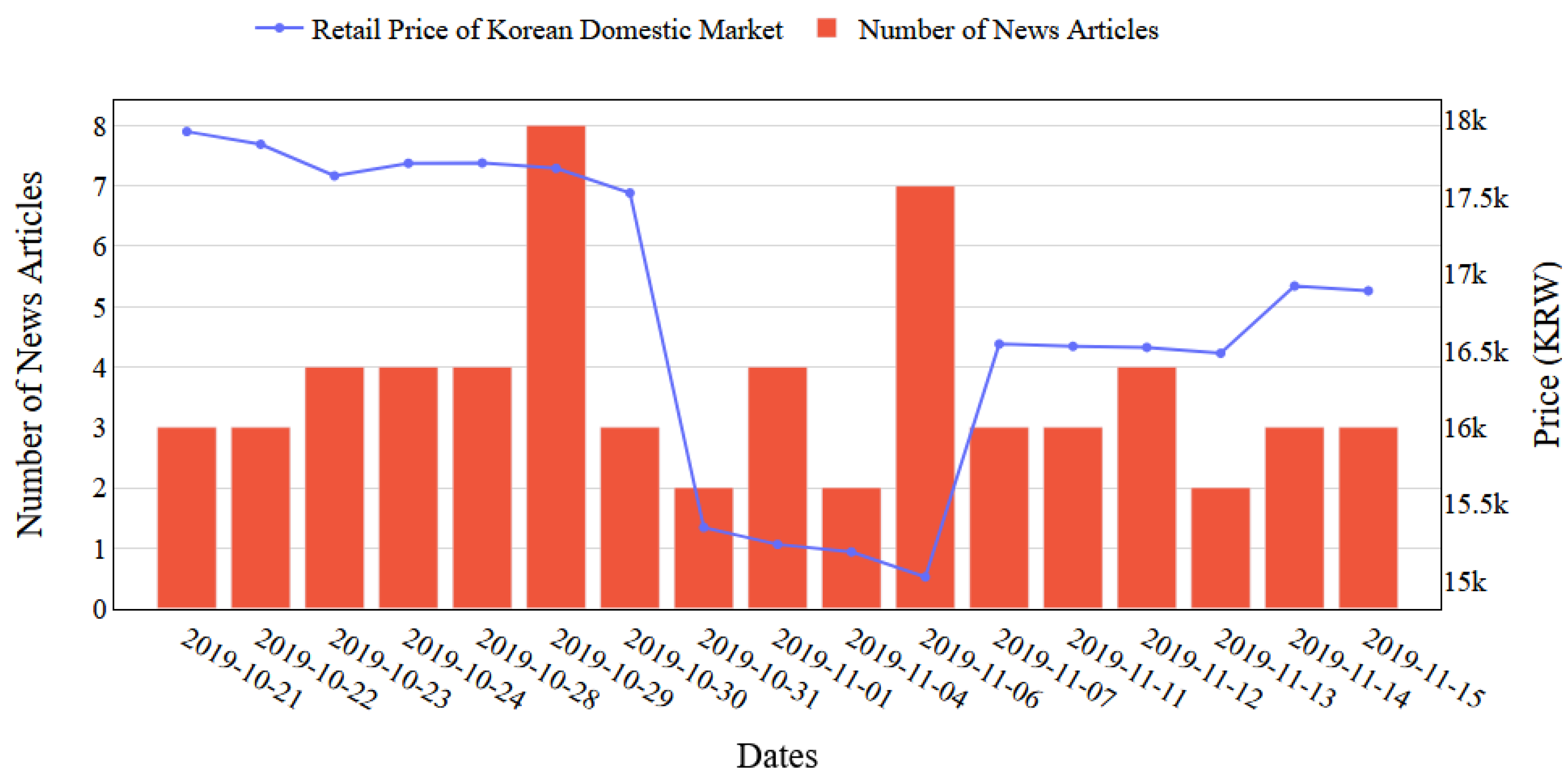
Figure 1 demonstrates how the news articles can affect the price (in our case, Korean Won, KRW) of a livestock commodity (in our case, pork). From the figure, we can observe that the price dropped after the number of news articles suddenly increased on October 29. Since that day, the price has been decreasing continuously. Again, on November 6, the number of news articles increased then the price increased.

Table 1. The result of topic modeling on news articles.

Date	Keywords
29 October 2019	Wild boar, Wild, Progress, Association, Technology, Representation, Industry, View, Virus, Africa, Fever, Occur, Detection, Farm, Ministry of Environment
6 November 2019	Association, Disposal, Policy, Duplication, Wild boar, Speed, Management, Disinfection, Effort, Execution, Prevention, Area, Corpse, Facility, Demand, Fixing

attempts to explain the reason for these price shifts. Specifically, Table 1 shows the result of topic modeling that produced relevant keywords from the news articles on certain dates. These relevant keywords help to understand the reason for various market conditions. For example, when the price decreased on October 29, there were topic keywords, such as “African swine fever”, “occur”, “virus”, and others. These words express that a disease associated with pigs had occurred. Owing to the disease, the price decreased continuously. On the other hand, when the price increased on November 6, there were topic keywords, such as “prevention”, “policy”, “management”, “disinfection”, and others. This may indicate that the government implemented policies to contain the spread of the virus.

1.3. Contributions

This paper focuses on predicting pork prices based on news articles by incorporating deep learning and topic modeling methods. Pork is one of the most frequently consumed livestock commodities in South Korea. The Ministry of Agriculture, Food and Rural Affairs (MAFRA) states that there are 11.7 M head of swine and 6137 farms in South Korea, and the trade of pork is second in terms of agricultural production value [20]. Moreover, pork is the most commonly consumed meat (i.e., 27 kg, annual per capita) in South Korea [20]. Meat consumption statistics provided by the FAO (2020) confirm that pork consumption is much higher than the rates for other types of meat in South Korea, with poultry, beef, and mutton in second, third, and fourth place, correspondingly [21,22].

To predict pork prices accurately, we first extract important topics of news articles related to pork and allocate a relevant topic to each news article. We then use a single-layer, the long short-term memory (LSTM) [23,24], a well-known algorithm for analyzing time-series data, to predict agricultural commodity prices by learning topics of news articles. The experiments are designed and conducted based on the last decade of South Korean news articles and price datasets pertaining to pork. Precisely, the contributions of this paper are as follows:

• We first propose the implementation of a topic modeling method, called latent Dirichlet allocation (LDA) [25,26], to obtain relevant keywords from the news articles. LDA uses word probability distributions in text data to retrieve a set of main keywords called a topic. LDA contributes to the goal of this paper in that (1) a number of topics are generated from news articles, (2) relevant topics are allocated to each news article, and (3) keywords associated with price fluctuations are extracted.
• Furthermore, we use a single-layer LSTM to predict agricultural commodity prices based on the topic modeling results. For this, we first convert the result of the topic modeling with LDA into a term frequency/inverse document frequency (TF-IDF) model. TF-IDF produces the numerical representation of keyword importance in topics, which is used as the input to the LSTM model along with the price of agricultural commodities. Considering that the data we used are a time-series, LSTM enables us to recognize patterns in the data over a long period.
• We evaluated the performance of the proposed approach through extensive experiments with state-of-the-art statistical (ARIMAX and ridge), machine learning (random forest and gradient boosting), and deep learning methods (multilayer perceptron and convolutional neural networks). The experimental results show that the proposed approach using LSTM greatly reduces the error rate compared to those resulting from the state-of-the-art methods.

1.4. Literature Review

In this section, we review related studies that focus on price predictions of agricultural commodities. We can roughly classify these studies into the following four categories: (1) studies that use structured data; (2) studies that use unstructured data; (3) studies that use both unstructured and structured data together; and (4) other studies. Subsequent sections discuss each category in detail.

1.4.1. Prediction of Agriculture Commodity Price Using Structured Data

There have been several studies, such as those by Liu et al. [27] 2019, Zhang et al. [28], Xiong et al. [14], and Li et al. [29], who predicted the prices of agricultural commodities using structured data. The similarity of these studies is that they used various data decomposition strategies and divided the data into the trend, seasonal, and cyclic components. For example, Liu et al. [27] proposed a hog price prediction method using a combination of a similar sub-series search and support vector regression (SVR) methods. The authors initially decomposed the dataset into the so-called trend and cyclical components of hog price data. Here, the trend component represents a long-term pattern, and the cyclical component represents the up and down movements of the pattern. Afterward, the authors predicted the trend component using SVR and the cyclical component using the most similar sub-series search method. The experiments were conducted using a dataset from a Chinese agricultural website from 2011 to 2017. The experiment results demonstrate that the proposed method is suitable for predicting the prices of hogs along with other agricultural commodities. Li et al. [29] applied a short-term prediction model of weekly retail prices for eggs based on a chaotic neural network. Considering its higher accuracy than traditional time-series models, the chaotic neural network model is a good tool for short-term forecasts of non-linear time-series data. The experiments were designed using a dataset from 2008 to 2012 in China, where the authors compared their outcomes with a well-known statistical algorithm, autoregressive integrated moving average (ARIMA). The results showed that the chaotic neural network is more accurate than ARIMA.

Some studies used hybrid learning methods to predict the prices of agriculture commodities. For example, Xiong et al. [14] predicted agricultural commodity prices using hybrid seasonal-trend decomposition procedures based on Seasonal Trend Loess (STL) and extreme learning machines (ELM) methods. The STL method was used to decompose the dataset into several components, referred to there as the seasonal, trend, and remainder components. Afterward, the ELM method was used to predict the outcomes related to these three components separately. The experiments in their paper were conducted using evidence pertaining to Chinese market vegetables, such as peppers, cucumbers, green beans, and tomatoes. The experiments demonstrated that the STL-ELM model showed higher accuracy on the seasonality component than the trend and remainder components. Zhang et al. [28] proposed a novel agricultural commodity price prediction model based on fuzzy information granulation and the mind evolutionary algorithm/support vector machine (MEA-SVM) model. Their work selected the time series data of the FAO food price index, a measure of the monthly change in the international prices of food, meat, dairy, cereals, oils, and sugar. First, the authors decomposed the price index dataset into the trend component using the fuzzy information granulation method. Afterward, a combination of a mind evolutionary algorithm and support vector machine was employed to forecast food price indexes. Their research showed that the MEA-SVM model is useful for predicting food price indexes.

1.4.2. Prediction of Agriculture Commodity Price Using Unstructured Data

There have been several studies [12,30,31,32,33] who predicted the prices of agricultural commodities using unstructured data, such as news articles, social network data, and others. Here, researchers have sought to predict prices using text analysis methods such as sentiment analysis and topic modeling.

Twitter data are widely used in the research on price predictions of agricultural commodities (Kim et al. [12], UN Global Pulse. [30]; Surjandari et al. [31]) because millions of users share their opinions on this platform [12,30,31]. For this reason, Twitter data are playing an important role in the analysis of public opinions. Kim et al. [12] proposed a two-step algorithm for the “nowcasting” of commodity prices using social media. In the first step, they extract tweets mentioning price quotations of the four food commodities, such as beef, chicken, chili, and onion. The second step is to build a statistical model to nowcast the prices. To be precise, they nowcast the current day’s prices using the previous day’s official market prices and the prices from tweet quotations. They predict prices with a mean absolute percentage error (MAPE) range of 4–32%. The authors observed that when the number of tweets about food prices increase, food prices change sharply. Surjandari et al. [31] also used Twitter data for public sentiment analysis of staple food price changes. Specifically, their experiments were conducted using stable food prices in Indonesia based on Twitter data. The authors first used sentiment analysis for classifying tweets into positive and negative sentiment. They then applied state-of-the-art classification algorithms to analyze the association between the type of staple food and the sentiment class, with the results showing that the SVM classifier produces higher accuracy than naive Bayes and the decision tree methods. They noted that the prices of milk, eggs, and red onions are significantly associated with negative sentiment compared to other commodities.

Recall from Section 1.2 that news articles represent one of the main channels for sharing updates about events related to agricultural commodities. Thus, another approach to predict agricultural commodity prices using unstructured data is from news articles. For example, Chakraborty et al. [16] proposed a novel generative model of real-world events and employ it to extract events from a large corpus of news articles. The authors grouped events by event triggers, which are specific words that describe the events. The extracted events were used to predict the prices of 12 different crops. They showed that their model reduces the root mean squared error (RMSE) of predictions by 22% compared to the standard ARIMA model. On the other hand, Yoo [32] introduced a vegetable price prediction method using atypical web-search data and a Bayesian structural time series (BSTS) model. The author collected related web-search data from Google and Naver associated with the South Korean wholesale vegetable markets for garlic, onion, and dried red pepper at the monthly level. The text data were then converted to numeric representations using the TF-IDF, after which the BSTS model was applied to the dataset. The experiment results demonstrated that atypical web-search data can improve the price prediction and that the improvement across BSTS models could differ according to the types of vegetables analyzed.

1.4.3. Prediction of Agriculture Commodity Price Using Unstructured Data and Structured Data

In this approach, unstructured data and structured data are used together to achieve high accuracy in price prediction. For example, Ryu et al. [33] introduced forecasts of the purchase amounts of pork using structured and unstructured data. Specifically, this research aimed to forecast consumption of pork using unstructured data, such as online text news, blogs, and television programs/shows. Here, the authors selected statistical information (e.g., news articles frequency, number of emotions, number of comments, blog frequency) from the unstructured data as the input/features of the prediction models. In addition to the unstructured data, the authors also used structured data (e.g., consumer panel data, retail and wholesale prices). Their experiments were constructed and trained using a South Korean market dataset from 2010 to 2016. To evaluate the study, they use statistical methods (autoregressive exogenous model, vector error correction model), machine learning methods (gradient boosting and random forest), and LSTM. LSTM shows the least error accuracy from these models. The results demonstrated that there is a relationship between pork consumption and unstructured data such as that found in news articles and blogs.

1.4.4. Other Studies

There have also been studies based on classical econometric methods [10,11,34,35]. For example, Zafeiriou et al. [34] aimed to examine the relationship of crude oil corn and crude oil soybean future prices using the autoregressive distributed lag (ARDL) co-integration approach. Their findings on the data from July 1987 to February 2015, derived from Bloomberg, confirm that crude oil prices affect the prices of agricultural commodities. Vo et al. [35] studied the relation between agricultural commodities prices and oil markets using demand and alternative oil shocks. The authors used the structural vector autoregressive (SVAR) model to investigate how the confusions to agricultural markets contribute to the crude oil prices. The paper results show that the crude oil market can be an affection in fluctuations in agricultural commodity prices. Drachal [11] analyzed the agricultural commodity prices with novel Bayesian model combination schemas. The analysis was made on wheat, corn, and soybean data from 1976 and 2016. In particular, a one-month ahead forecast was achieved with the dynamic model averaging (DMA) and Bayesian model averaging (BMA) that outperforms some conventional econometric models, such as ARIMA, historical average, or the naïve method. In addition, the findings of the research indicate that the initial price drivers were various fundamental, macroeconomic, and financial factors. Vu et al. [10] conducted an examination of the transmission mechanisms that influence the relationship between oil and agricultural prices. The authors analyzed ten agricultural commodities from 2000 to 2019 using the interacted panel vector autoregressive framework and investigated the effect of biofuel production. The authors declared that oil prices could affect agricultural prices through biofuel and exchange rates.

2. Materials and Methods

2.1. Overview

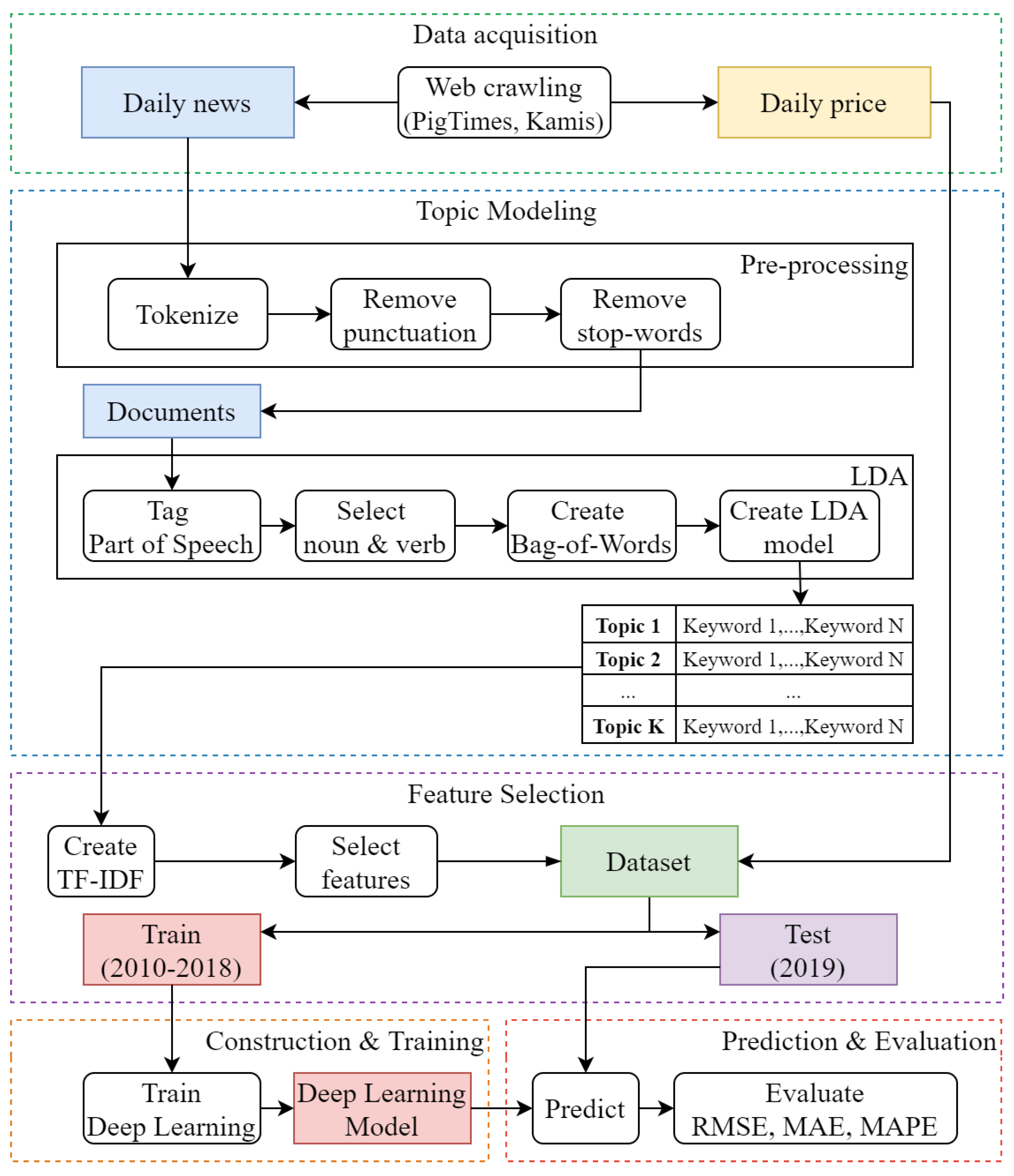
Figure 2 describes the overall flow of the proposed approach. It consists of the following steps: data acquisition, topic modeling, preprocessing, feature selection, model training, and accuracy testing of the model. We mainly intend to predict the retail price of pork in the South Korean domestic market using daily news articles. The datasets were obtained from various online source using web crawling techniques. Afterward, the main topics were extracted from the dataset using a topic modeling technique called LDA. Based on the extracted topics, we predict the retail prices of pork using LSTM. Finally, we measure and compare the error accuracy of the proposed method with state-of-the-art statistical, machine learning, and deep learning models. In the subsequent subsections, we will describe each step in detail.

2.2. Data Acquisition

Recall from the previous section that we predict the retail price of pork based on daily news articles. For this, we collected news articles from an Internet source using web crawling techniques. Web crawling refers to a process by which we first load web pages using their URLs, parse the error accuracy contents, extract the pages to the XML or HTML formats, and store them in a database. The web crawling technique enables us to obtain a massive amount of data from online web pages. There are many options and methods one can use to crawl websites. In our case, we used the Python 3 packages, such as Requests and Beautifulsoup. Here, while the Requests package enables us to send an HTTP request and receive a related response, the Beautifulsoup package easily perceives the contents of HTML and XML files.

There are three types of sources that we used in this paper: PigTimes [36], Korea Agricultural Marketing Information Service (KAMIS) [37], and Livestock Product Quality Evaluation Center (EKAPEPIA) [38]. PigTimes is a South Korean online news website that publishes only news articles about pigs and pork and their market conditions on a daily basis. One problem associated with crawling data from the Internet is that we do not know if the content is related to the keyword. For example, we can find news article using the “pork” keyword, but it is important to confirm that the news article is actually related to pork. Because our data source is related only to pork, this type of problem does not arise, which is why PigTimes was chosen. News articles were collected from 2010 to 2019. Afterward, we collected a price dataset from KAMIS, which is a website that provides various information related to the distribution of agricultural and livestock commodities in South Korea. From KAMIS, we collected the daily retail price of pork from 2010 to 2019.

Table 2. The details of collected dataset.

Website	Content	Amount	Date
PigTimes	News articles from South Korea related to pig, pork, farm, market, disease, etc.	10,854	January 2010–December 2019
KAMIS	Daily pork retail price in South Korea	2466
	Daily market price in South Korea	2466
	Daily distributor price in South Korea	2466
EKAPEPIA	Daily auction price in South Korea	2909

KAMIS: Korea Agricultural Marketing Information Service; EKAPEPIA: Livestock Product Quality Evaluation Center.

shows the detailed information of the datasets used here. There are 10,854 daily news articles and 2466 daily prices, excluding weekends.

2.3. Topic Modeling

2.3.1. Implementation of the LDA Model

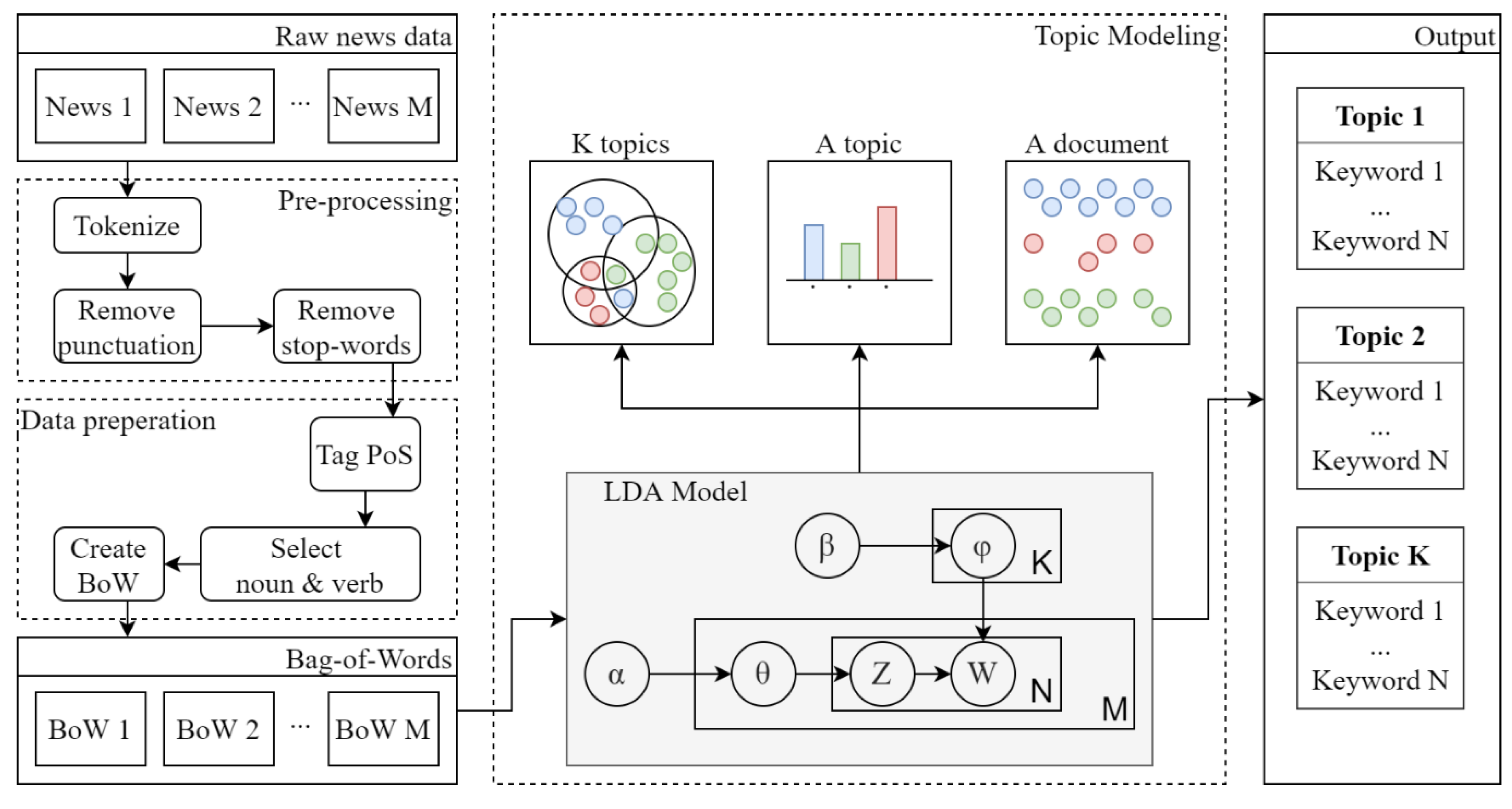
The main feature of topic modeling is to extract the main keywords, which express the overall meaning of news articles. In other words, topic modeling is a type of natural language processing (NLP) model for extracting abstract topics from text data. LDA is a popular topic modeling algorithm. Figure 3 describes the implementation of LDA for our dataset. In the implementation of LDA, there are three main steps: data cleaning, modeling, and output. Data cleaning consists of two steps, such as tokenization, punctuation and stop-word removal. Tokenization is the way to extract sentences to words. Specifically, it converts a sentence into a collection of words. Afterward, the stop words are removed from the collection. Stop words are words that commonly appear but do not have an effect on the meanings of the sentences.

After the data cleaning process, we extract words according to their parts of speech using KoNLPy [39], which is a Python package for NLP of the Korean language, selecting only nouns and verbs, as nouns and verbs can express the principal meaning of a sentence. The KoNLPy has several options for tagging words by part-of-speech (PoS) and open Korea text (Okt). In this paper, we selected Okt, as it allows stem tokens, meaning that we can obtain a root word without any inflectional affixes. Subsequently, a bag-of-words (BoW) model was created using the result of PoS tagging. The BoW model is the numerical representation of text data. The “bag-of-words” includes information such as the ID and the occurrence of words in a document. Accordingly, we can apply the LDA model using the BoW model.

The LDA model part in Figure 3 shows the plate notation for the LDA model, and Equation (1) represents the plate notation [25,40]. In Equation (1), we first initialize the parameters (i.e., the parameter of the Dirichlet prior to the per-document topic distributions, and parameter of the Dirichlet prior on the per-topic word distribution). On the left side of the equation is the probability that the topic will appear. There are four factors on the right side of the equation, with the first two being Dirichlet distributions and the last two multinomial distributions. The first factor represents the probability that a document will be relevant to the topic. The second factor indicates that topics are associated with words. The third factor means that words in the document will belong to a topic. The last factor indicates that words are associated with a topic.

$$P\left(W,Z,\theta ,\phi ,\alpha ,\beta \right)={\displaystyle \prod }_{j=1}^{M}P\left({\theta }_j;\alpha \right){\displaystyle \prod }_{i=1}^{K}P\left({\phi }_i;\beta \right){\displaystyle \prod }_{t=1}^{N}P\left(Z_{j,t}|{\theta }_j\right)P\left(W_{j,t}|\phi Z_{j,t}\right)$$

(1)

In the plate notation and Equation (1), the following notations are defined as follows:

• $M$: Number of documents.
• $N$: Number of words in a document.
• $K$: Number of topics.
• $W$: A word in a document.
• $Z$: A topic assignment in a word.
• $\theta$: A topic distribution for a document.
• $\phi$: A word distribution for a topic.
• $\alpha$: The Dirichlet-prior concentration parameter of the per-document topic distribution.
• $\beta$: The Dirichlet-prior concentration parameter of the per-topic word distribution.

The LDA model returns $K$ number topics, which include $M$ number of words. It is necessary to set $K$ manually, and this is a limitation of the LDA method, as the result of the LDA model changes greatly depending on the number of topics. We applied the LDA model with a few different numbers of topics and selected the optimum case.

2.3.2. LDA Model Results

This subsection discusses the result of the LDA model. We applied the LDA model to obtain relevant topics from more than 10,000 news articles.

Table 3. Topics discovered from more than 10,000 news articles using LDA.

Agreed Topic	Frequent Keywords (Translation)
Import	Increment, Import volume, Prospect, Consumption, Shipment, Emphasis, Level, Shipment volume, Import, Decrement
Disease	Foot-and-mouth disease, Occurrence, Vaccination, Price, Record, Decrement, Support, Release, Farm, Import volume
Farmhouse	Conduct, Sales, Farm, Agriculture feed, Supply, Feed, Productivity, Photography, Promotion, Education
Market	Import volume, Price, Income, Propel, Analysis, Occurrence, Conduct, Record, Production, Market
Government	Inspection, Penalty, Conduct, Reinforce, Proceeding, Government, Levy, Remove, Ministry of Agriculture, Food and Rural Affairs, Confirm
Price	Price, Decrement, Increment, Record, Attainment, Propel, Output, Income, Hold, Increment

describes the top six topics, in this case, imports, disease, farmhouses, markets, governments, and prices. The LDA model returns the topics with their keywords, but without labeling them. It is necessary to analyze the topics and label them using similar words. For example, the first topic can be labeled as “Imports”, because there are keywords such as import volume, import, shipment, and shipment volume.

2.4. Feature Selection

The result of the LDA model consists of K number of topics, which include M number of words. Using this result, we first established the best topics for each news article. Afterward, the TF-IDF model was applied and combined with the price data to create the dataset for the prediction models. Finally, we applied the feature selection method to retrieve the features that were more correlated with the price.

It is important to note that topic modeling produces hundreds of features in the model training set. Having too many features adversely affects the results. For example, it increases the calculation time and decreases the accuracy of the result, as it includes some words that are not related to the prediction output. Choosing the right feature selection method depends on the input and output variables. We chose Pearson’s correlation in this paper, because we have numerical input and numerical output. Pearson’s correlation determines the linear relationship between two variables using a number between −1 and 1. Here, −1 represents a negative relationship, 1 represents a positive relationship, and 0 means there is no relationship. Equation (2) describes the Pearson’s correlation. In the equation, $r$ represents the correlation, and $n$ represents the number of total values. Besides, $x$ and $y$ represent two values that are correlated.

$$r=\frac{n\left({\displaystyle \sum }xy\right)-\left({\displaystyle \sum }x\right)\left({\displaystyle \sum }y\right)}{\sqrt{\left[n{\displaystyle \sum }{x}^2-{\left({\displaystyle \sum }x\right)}^2\right]\left[n{\displaystyle \sum }{y}^2-{\left({\displaystyle \sum }y\right)}^2\right]}}$$

(2)

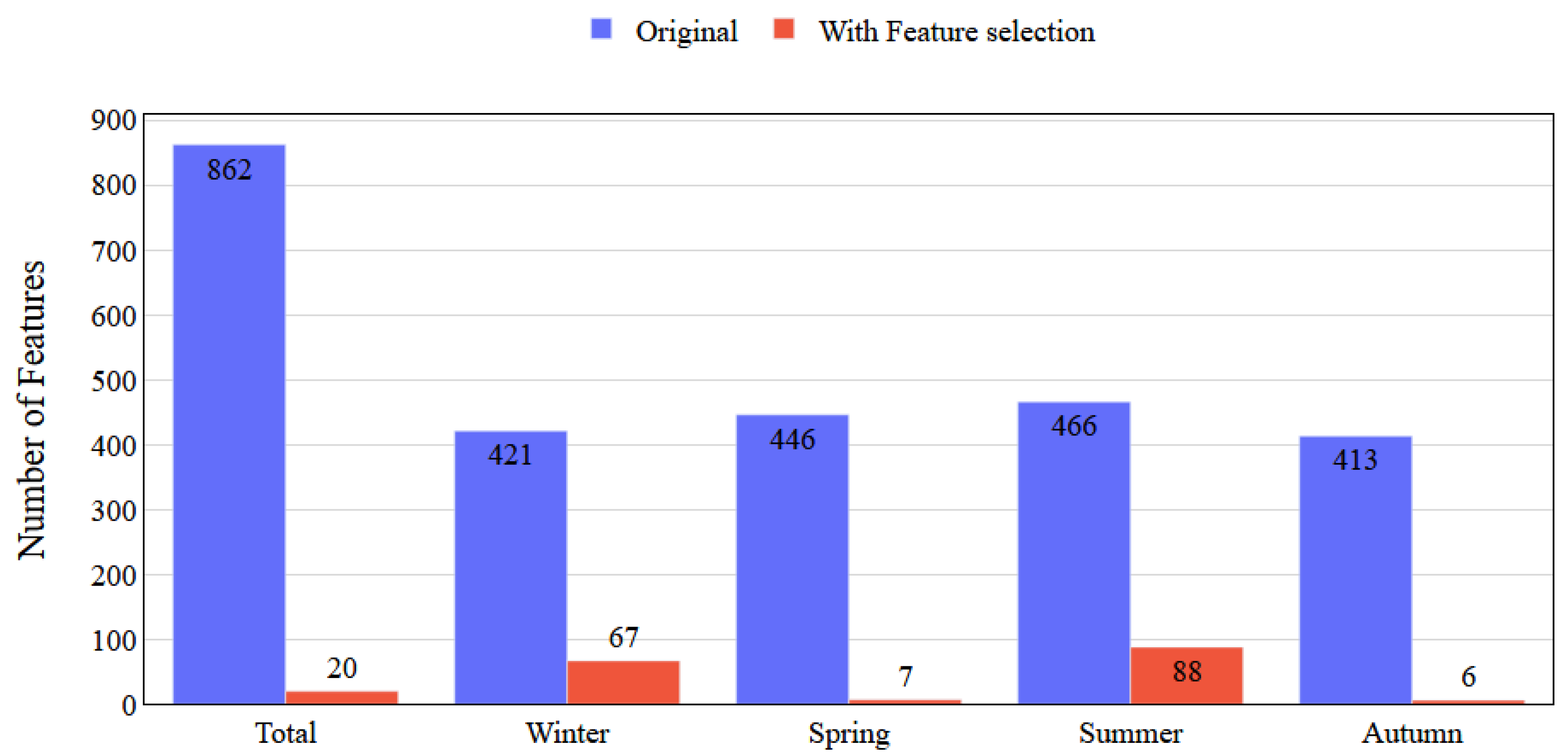
Figure 4 shows the number of features without and with the feature selection model. We calculated the correlation between the prices with all other features and selected the features that have a correlation of more than 0.01. The feature selection method was applied to five different datasets. It decreased the number of features by more than 80%.

2.5. Price Prediction with Deep Learning

In this paper, we predict the retail price of pork using the LSTM algorithm in comparison with other methods. The LSTM algorithm is our principal method. Long short-term memory networks (LSTM) are a type of recurrent neural network (RNN) [41]. Basic RNNs have loops with which they combine with past data to solve a problem. In other words, RNNs find the solution to a task using previous data. The accuracy of the RNN model depends on the gap between the past information and the present problem. Accordingly, if the gap size grows, these methods are unable to solve the problem. We call this difficulty as long-term dependencies. It is a significant advantage that LSTM approaches avoid this difficulty.

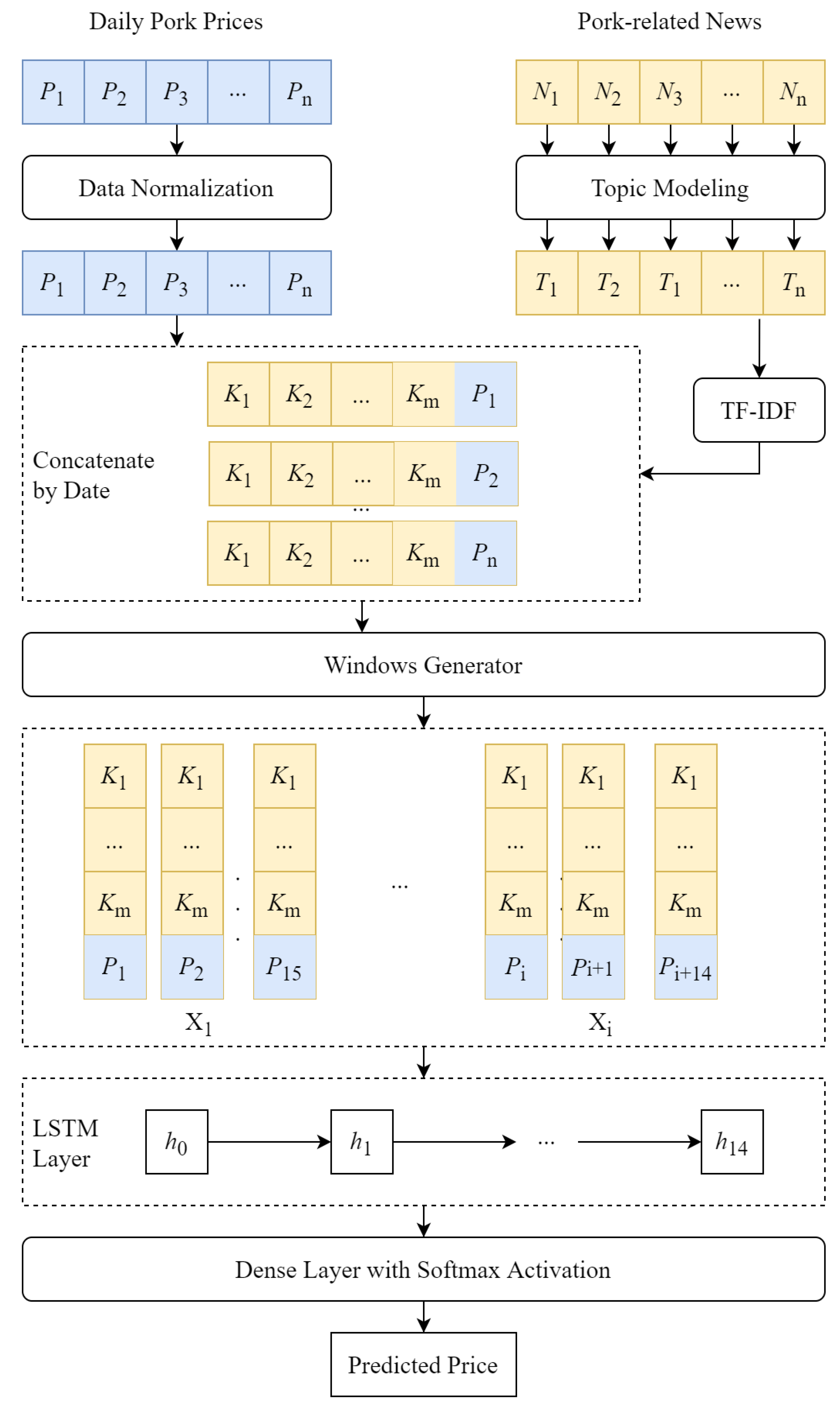
Figure 5 shows the process of price prediction with LSTM. In the figure, P, N, T, and K represent price, news, topic, and keyword, respectively. First, we converted the result of the LDA model into a TF-IDF model. This model represents the importance of keywords. In the model training step, LSTM requires a three-dimensional structure containing the number of samples, the number of time steps, and the number of variables. Thus, it was necessary initially to convert the dataset into this type of three-dimensional structure. In our case, the first dimension represents the size of the training data, the second dimension represents the size of the WINDOW component, and the third dimension represents the number of features. Afterward, we created a basic LSTM. It uses two types of layers, a single hidden layer of LSTM units and an output layer used to make a prediction. Additionally, we use one additional layer called a dense layer, which is a matrix-vector multiplication. Precisely, the dense layer was used to update the parameters of the model during the training step. This process uses the dataset and consists of data splitting, data preprocessing, and feature selection. The dataset is the data that came from the TF-IDF model, which in turn came from the result of the LDA model and the retail price of pork. The dataset was split seasonally to enhance the result of the prediction.

The LSTM cell consists of three types of gates: a forget gate, an input gate, and an output gate. The forget gate is for removing information that is no longer required or less required for predictions from the cell state. This action optimizes the performance of the LSTM. The input gate adds new information to the cell state. The LSTM selects the output and shows it using the output gate. These gates are correspondingly described by Equations (3), (4) and (6). Equation (5) calculates the present cell state and Equation (7) calculates the output of the LSTM model.

$$f_t=\sigma \left(W_f\left[h_{t-1},X_t\right]+b_f\right)$$

(3)

$$i_t=\sigma \left(W_i\left[h_{t-1},X_t\right]+b_i\right)$$

(4)

$$C_t=\tanh \left(W_c\left[h_{t-1},X_t\right]+b_c\right)$$

(5)

$$o_t=\sigma \left(W_o\left[h_{t-1},X_t\right]+b_0\right)$$

(6)

$$h_t=o_t\ast \tanh \left(C_t\right)$$

(7)

In the equations above, $f_t$, $i_t$ and $o_t$ correspondingly represent the forget gate, the input gate, and the output gate in the time step $t$. $X_t$ is the input to the cell layer at time step $t$. $W_f$, $W_i$ and $W_o$ are the weight matrices, and $b_f$, $b_i$ and $b_o$ are the bias vectors.

3. Results

3.1. Experimental Setup

This subsection describes the properties of the machine used for the experiments. The machine runs with an Intel (R) Core (TM) i9-9900K 3.60 GHz CPU, a NVIDIA GeForce RTX 2080 GPU, and 32 GB of memory. We also installed the Windows 10 Home OS by Microsoft on the machine. All developments and experiments were implemented in the Python (Version 3.7.6) programming language and its packages. The dataset used with the experiments was collected using web crawling packages, specifically Requests (Version 2.22.0) and Beautifulsoup (Version 4.9.0). We applied text mining methods using the NLP packages of KoNLPy (Version 0.5.1) and Gensim (Version 3.8.0), while the price prediction models were applied using the packages Scikit-learn (Version 0.21.3) and Keras (Version 2.2.5). The visualizations of all experiments were shown by Plotly (Version 4.6.0). Section 3.1.1 describes the dataset used in the experiments. In Section 3.1.2, we compare the LSTM with other statistical and machine learning algorithms. Section 3.1.3 describes the accuracy metrics used to evaluate the results.

3.1.1. Dataset

This paper uses two types of datasets: structured (retail price) and unstructured (news articles) from January 2010 to December 2019. The news articles were collected from PigTimes, and the retail prices of pork were from KAMIS. Both datasets cover the South Korean domestic market.

Table 4. Summary of datasets used in experiments (from January 2010 to December 2019).

Statistics	Amount	Mean	Maximum	Minimum	Standard Deviation
Daily retail price	2466	18,747.58	25,287	11,332	2426.65
Daily news articles	10,854	9.1	29	1	6.3

summarizes the statistical information of the retail price and news articles. From the table, we can see that there are 2466 data instances related to the daily retail price of pork, excluding weekends. We can also observe that the average retail price of pork is KRW 18,747, and the standard deviation indicates that consumers buy pork between KRW 16,320 and KRW 21,174 in most cases. We also collected a total of 10,854 news articles related to pork.

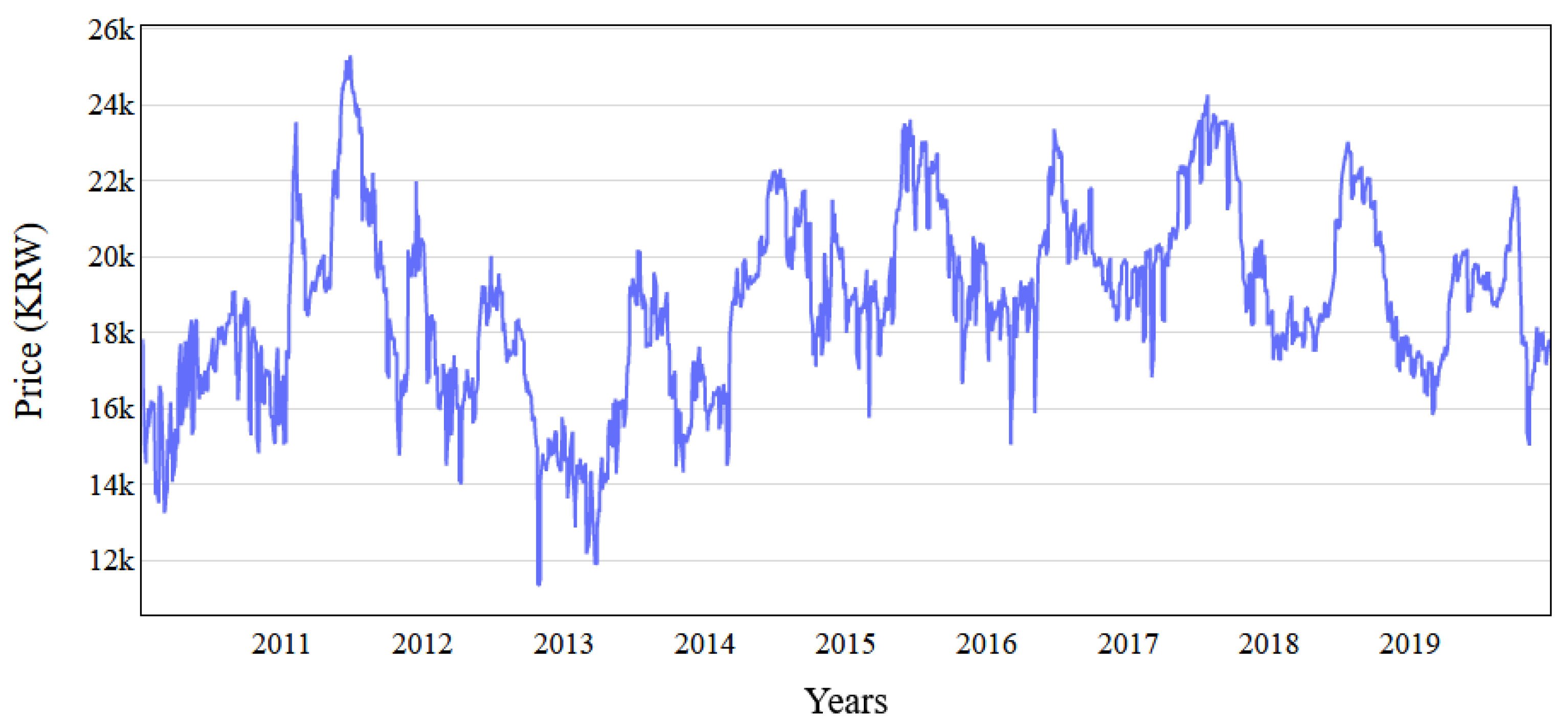
Figure 6 shows the time-series data on retail pork prices. This figure explains the distribution of the pork price. For example, there is a seasonal pattern by which the price in the middle of each year increases. The seasonal pattern expresses that there is a relationship between seasons and prices. Thus, we increased the accuracy of our prediction model by splitting the dataset into different seasons.

The collected dataset used here contained data from 2010 to 2019. To build and train the prediction models, a training dataset from 2010 to 2018 was used. The remaining data were used for testing the prediction models. Specifically, we predict the data for 2019 using data from 2010 to 2018.

Table 5. Summary of seasonal dataset.

Season	Months	Total	Train Size	Test Size
Winter	Dec, Jan, Feb	282	234	48
Spring	Mar, Apr, May	293	245	48
Summer	Jun, Jul, Aug	304	260	44
Autumn	Sep, Oct, Nov	296	248	48
Total		1175	987	188

shows the number of datasets according to the season.

3.1.2. Competing Methods

As mentioned earlier, the LSTM approach was selected as our principal method. To compare our results, we also used other statistical and machine learning methods, in this case, the autoregressive integrated moving average (ARIMAX) method with an exogenous variable, ridge, random forest (RF), gradient boosting (GB), and statistical and machine learning methods, all of which are still major candidates in the prediction sector. Choosing the most appropriate model depends on the datasets used, and typically selecting the best option is challenging. Thus, we selected these methods to certify that LSTM is the best option for our dataset.

ARIMAX is an extension of the ARIMA model for a multivariate dataset, where the last X stands for exogenous variables. ARIMAX can predict stationary or non-stationary prices. In addition, it works with any type of data pattern, such as trends, seasonal patterns, or those containing cyclicity. This is why we selected the model as a statistical method for our experiments. Ridge regression is a regularization technique for linear regression models. Regularization is a technique that allows one to avoid the overfitting and underfitting of data and adds a parameter (alpha) for better results. A low alpha value can lead to overfitting, while a high alpha value can lead to underfitting. Random forest is a well-known supervised machine learning algorithm for classification and regression. Random forest can work with a dataset that has a large number of features. In addition, it presents the importance of variables. However, random forest is not well adapted for categorical data. Gradient boosting is a powerful algorithm in the area of classification and regression problems. Here, boosting means to combine multiple simple models into a single complex model. Therefore, gradient boosting uses the decision tree as a single model. Additionally, there are two types of deep learning methods: multi-layer perceptron (MLP) and conventional neural networks (CNN) [42]. MLP is a field of feedforward artificial neural networks, consisting of an input layer, hidden layer, and output layer. CNNs are widely used in the area of computer vision, but they can also be used for price predictions.

Table 6. Comparison of competing methods modified from [43].

Type	Method	Pros	Cons
Statistical	ARIMAX	- Simple to implement - Easier to handle - Quick to run	- High pre-requisites - Linear
Machine Learning	Ridge	- Simple to implement - Good interpretation - Prevent over-fitting	- Need to select perfect hyper parameter
	Random Forest	- Non-linear - Provides feature importance - Can handle missing values	- Easy over-fitting - Requires more computational resources - Prediction time is high
	Gradient Boosting	- Good interpretation - Prevents over-fitting	- Sensitive to outliers - Difficult to scale up
Deep Learning	MLP	- Non-linear - Flexible	- Depends on a lot of data
	CNN	- Non-linear	- Expensive computation

compares the prediction algorithms used here and presents their pros and cons.

3.1.3. Evaluation Metrics

To evaluate the performance of the proposed method, we compared the actual retail price of pork sales with the predicted price according to certain standard statistical measures. Specifically, we used root mean squared error (RMSE), mean absolute error (MAE), and mean absolute percentage error (MAPE) given in Equations (8)–(10), respectively. Here, $N$ represents the number of samples, $y$ represents an actual value, and $f$ represents a predicted value. RMSE is the standard deviation of the prediction errors. The absolute error calculates the difference between the actual value and the predicted value. Hence, MAE is the average of all absolute errors. MAPE calculates the average of the absolute percent error for each time. All measures indicate that lower values are better than higher values.

$$RMSE=\sqrt{\frac{1}{N}{\displaystyle \sum }_{i=1}^N{\left(y_i-f_i\right)}^2}$$

(8)

$$MAE=\frac{1}{N}{\displaystyle \sum }_{i=1}^N\left|y_i-f_i\right|$$

(9)

$$MAPE=\frac{1}{N}{\displaystyle \sum }_{i=1}^N\frac{\left|y_i-f_i\right|}{y_i}\ast 100$$

(10)

3.2. Experimental Results

This subsection presents the results of the experiments. We predict the daily retail price of pork using LSTM and the other statistical and machine learning algorithms. Afterward, the prediction models were evaluated using common error metrics, in this case RMSE, MAE, and MAPE. We utilized a dataset covering a decade from 2010 to 2019. The data from 2010 to 2018 were used to construct and train the models. Then, we tested the models using data from 2019. Section 3.2.1 compares the results of the models. Section 3.2.2 shows the impact of feature selection. Section 3.2.3 compares the parameters of the LSTM model. Section 3.2.4 presents the results of the experiments with LSTM using different types of prices. Section 3.2.5 summarizes the experimental results.

3.2.1. Hyperparameters of Competing Methods

Table 7. Hyperparameters of LSTM.

Case No.	Hyperparameters				Errors
	Window	Batches	Epochs	Learning Rate	RMSE	MAE	MAPE
1	10	32	30	0.001	1152.886	917.175	5.105
2	20	32	30	0.001	1195.985	977.666	5.378
3	15	32	30	0.001	1057.874	822.069	4.564
4	15	32	15	0.001	1254.486	1031.557	5.716
5	15	32	45	0.001	1109.823	904.309	5.012
6	15	64	30	0.001	1033.131	811.057	4.498
7	15	128	30	0.001	1042.166	820.804	4.551
8	15	256	45	0.001	1200.07	977.025	5.37
9	15	32	30	0.002	1007.432	793.786	4.411

RMSE: Root Mean Squared Error; MAE: Mean Absolute Error; MAPE: Mean Absolute Percentage Error.

shows the results of the experiments of the LSTM model with different values of the hyperparameters. LSTM uses windows, batches, epochs, and the learning rate as hyperparameters. LSTM is not overly sensitive to changes in these parameters, but the LSTM result could be improved by making slight changes in these parameters. Various combinations of the parameters were applied in the experiments, and the most optimum set was selected. We show several parameter configurations that led to better results in Table 7. In addition,

Table 8. Hyperparameter settings of the competing methods.

Algorithm.	Parameters
ARIMAX	Order	(2, 0)
	Trend	C
Gradient Boosting	Learning rate	0.1
Random Forest	Max depth	2
Ridge	Alpha	1
CNN	WINDOW	15
	Batches	32
	Epochs	30
MLP	Batches	32
	Epochs	30

shows the parameters of other state-of-the-art methods. We implemented each method with several combinations of parameters and selected the best options.

3.2.2. Comparison of Models

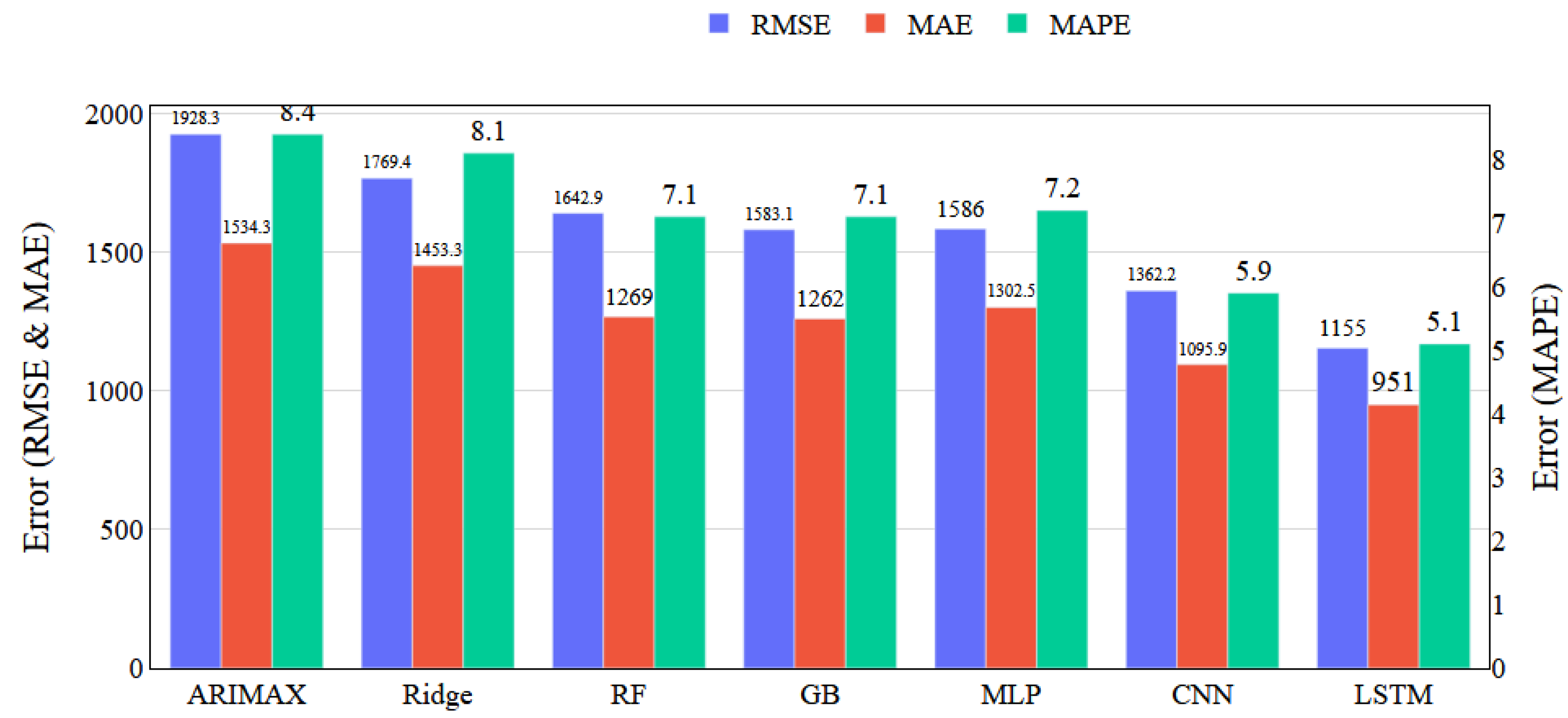
Figure 7 shows the results of all prediction models without feature selection. As shown in the figure, the result of the LSTM model shows the best accuracy. After the LSTM model, we can sort the models according to their error accuracy levels, as follows: gradient boosting, random forest, ridge, and ARIMAX. The result of the LSTM model was 37% lower than the result of the gradient boosting model, 42% lower than the result of the random forest model, 53% lower than the ridge model, and 66% lower than the ARIMAX model in terms of RSME. Additionally, the result of LSTM model was better than those of other deep learning models. Specifically, the LSTM model shows a result 28% lower than that by MLP and 16% lower than that by CNN in terms of RSME.

3.2.3. The Impact of Feature Selection

The next experiment sought to evaluate the impact of feature selection (FS). To improve our accuracy, the dataset was split into seasonal segments. In other words, we created models for each season, i.e., winter, spring, summer, and fall.

Table 9. Error rates of seasonal predictions.

Method	FS	Winter			Spring			Summer			Autumn
		RMSE	MAE	MAPE	RMSE	MAE	MAPE	RMSE	MAE	MAPE	RMSE	MAE	MAPE
ARIMAX	N	1632.58	1339.66	7.794	2026.26	1517.96	8.24	1367.86	1058.3	5.524	2584.98	2090.81	11.43
	Y	945.13	674.04	3.886	1564.20	1346.59	7.476	1306.25	1044.07	5.441	2002.71	1671.28	8.97
Ridge	N	782.49	618.20	3.603	1470.86	1275.36	6.932	1214.82	1055.83	5.504	2122.59	1814.63	9.87
	Y	503.63	404.62	2.351	1250.39	1025.58	5.496	878.01	745.47	3.884	1914.21	1592.49	8.57
RF	N	877.96	676.2	3.9	1423.09	1265.21	6.917	1937.23	1779.58	9.271	2249.16	1911.9	10.26
	Y	761.32	659.81	3.822	1327.57	1164.4	6.305	1440.6	1343.51	7.003	2187.89	1881.04	10.19
GB	N	892.57	701.55	4.069	1383.85	1193.71	6.427	1613.88	1476.4	7.689	2416.97	2063.34	11.19
	Y	844.2	648.23	3.772	1247.39	1078.4	5.861	1386.23	1252.02	6.517	2163.82	1766.88	9.63
MLP	N	854.8	667.86	3.902	1370.83	1210.933	6.535	1358.734	1228.29	6.401	2067.933	1780.033	9.775
	Y	590.25	485.67	2.827	1272.51	1048.872	5.606	918.371	787.305	4.102	1727.063	1415.169	9.938
CNN	N	618.12	506.444	2.957	998.688	883.155	4.675	1393.511	1347.59	7.043	1835.694	1545.803	8.659
	Y	609.4	500.296	2.606	732.04	532.632	2.838	977.969	838.566	4.383	1341.564	1079.776	5.912
LSTM	N	860.54	761.27	4.445	777.32	610.29	3.263	805.47	573.69	2.988	2276.48	2027.35	7.654
	Y	567.36	448.24	2.593	665.25	521.71	2.76	561.6	475.14	2.476	1264.15	1057.22	5.90

describes the detailed results in all seasons and methods. From the table, we can observe that LSTM outperforms most of the methods in terms of different accuracy metrics, such as RMSE, MAE, and MAPE. Even though we achieved high accuracy compared with state-of-the-art methods, there is still scope to improve the model. Particularly, there are many factors that impact the performance of the model. This can be also seen from Figure 6 that contains noises in time-series data on retail pork prices. These noises may reflect possible asymmetries in information concerning the media, the market, conflicts of interests, or opportunistic behaviors. In other words, there is a need for sophisticated data preprocessing methods that can further the accuracy of learning models. We will research data preprocessing methods in the future.

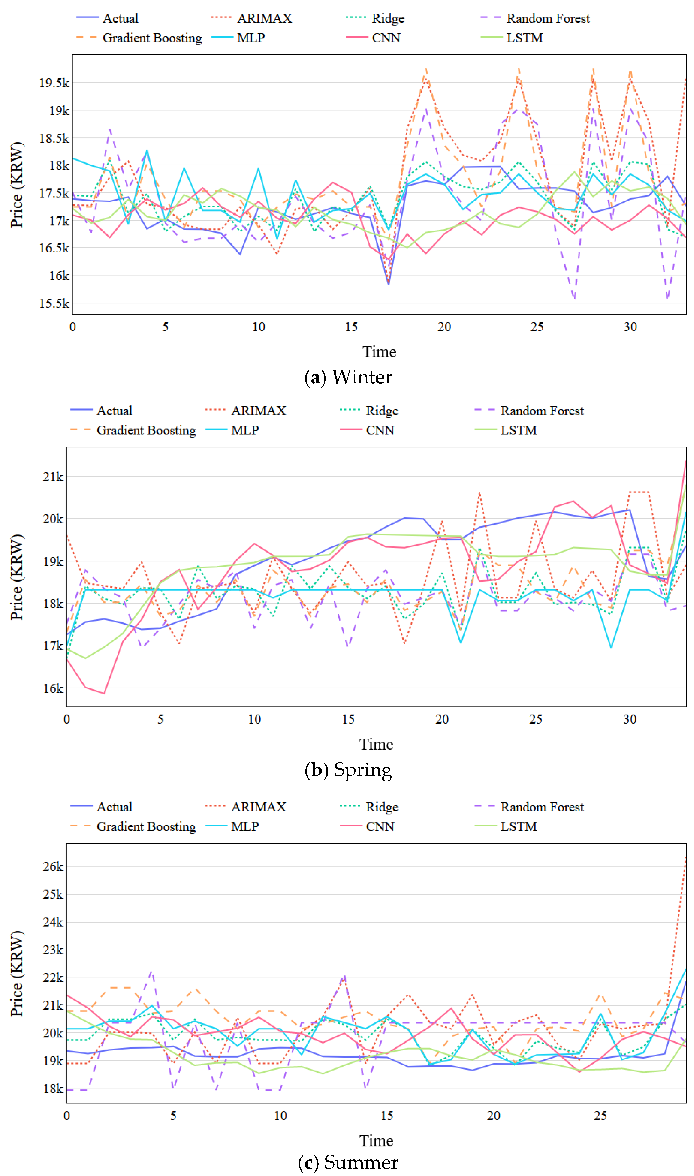
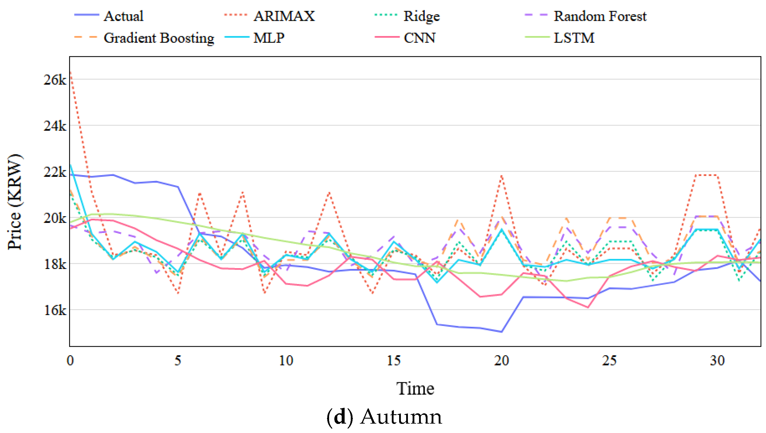
Figure 8 is a graphical depiction of Table 9 that displays the predictions of pork for a certain period of time. In the figure, the dark blue line represents the actual price, and the green line represents the prediction by the LSTM model. Here, it is clear that the prediction by the LSTM model follows the actual price better than those by the other models in all seasons. However, the results also demonstrate that accuracy is relatively lower in Autumn than other seasons. This is caused by the fact that there are many national holidays celebrated in South Korea in Autumn, which contribute to price fluctuations. In addition, there are other unexpected and unplanned events, such as the AFS outbreak in September 2019 [44], have impacted on prices.

3.2.4. Comparison of Different Types Prices

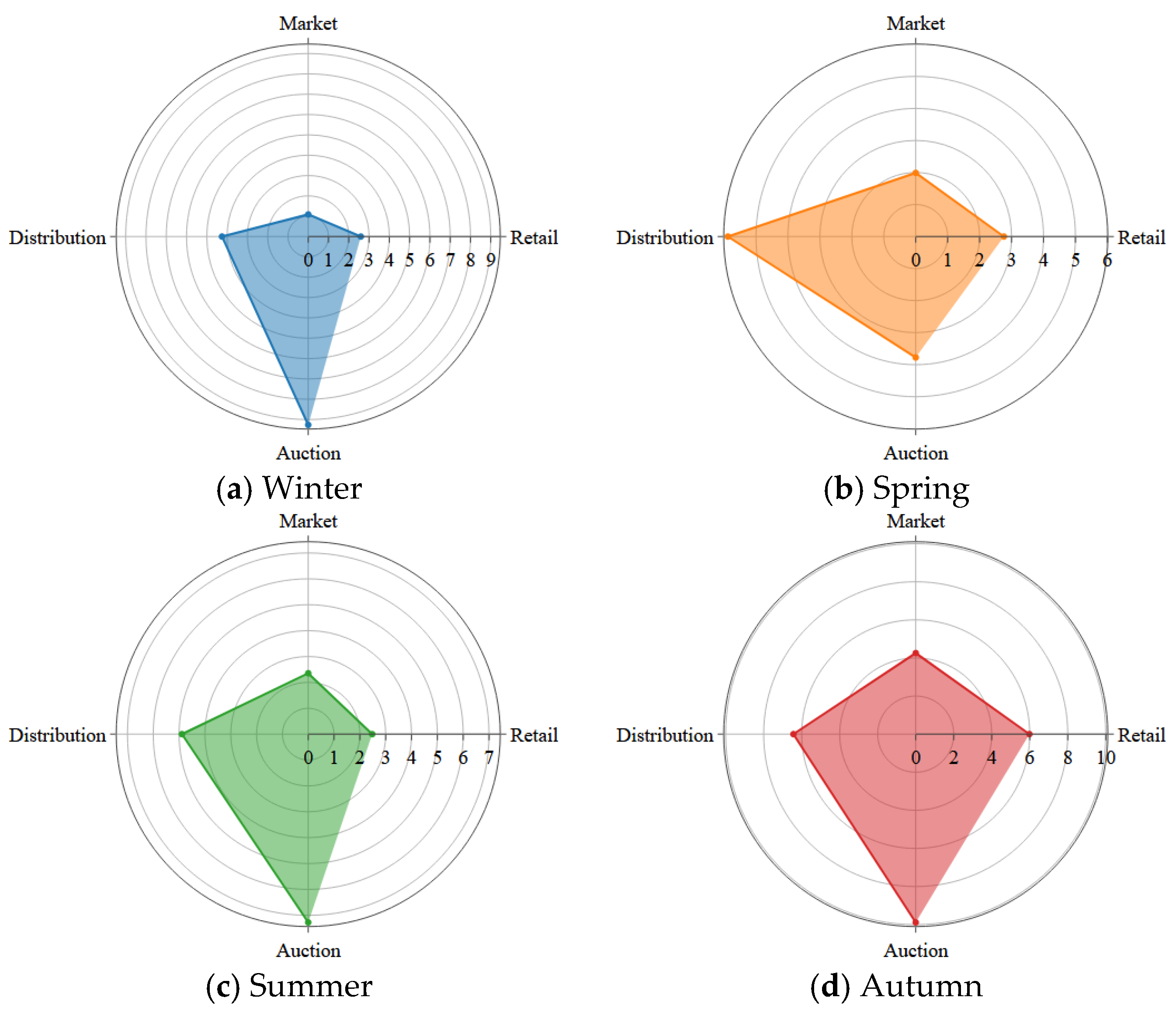
In this experiment, we applied the LSTM model with different types of prices. There are four types of price data, i.e., the retail price, marketplace price, distribution price, and auction price. The retail price is the price at which the end-user purchases pork. The marketplace price is the price at which pork is purchased in the South Korean traditional marketplace, unlike large supermarkets, such as COSTCO or HomePlus. The distribution price is the price at which large South Korean distributors such as Emart, Lotte Mart, and HomePlus sell pork, and the auction price is the price that is bid in the wholesale market. Figure 9 shows a comparison of the different types of prices by MAPE. Note that RMSE and MAE are not suitable for measuring the errors of different types of prices, as the prices are not in the same price ranges. In other words, the auction price is around KRW 5000, but other types of prices are close to KRW 18,000. Because MAPE represents the error percentage, the errors can be compared in this evaluation metric. From the figure, we find that the retail and market prices are similar in all cases. The result of the auction price is worse than the others, but for all MAPE outcomes, the errors are less than 10 percent.

3.2.5. Summary of Experiments

This paper proposed an approach to predict the daily retail price of pork based on news using LSTM. There are four types of experiments in this section. First, the LSTM model was compared with other statistical, machine learning, and deep learning models. Recall from Section 3.1.3, we compared the actual retail price of pork sales with the predicted price according to certain standard statistical measures. Specifically, we used RMSE, MAE, and MAPE given in Equations (8)–(10), respectively. The experiment results demonstrate that the LSTM performed better than these state-of-the-art models, showing at least 16% lower error rate. The second set of experiments sought to check the impact of the feature selection method. The number of features was reduced using Pearson’s feature selection method. The feature selection method could decrease the prediction errors, and the result of LSTM was best in all cases. Setting the most optimum parameters is important in all prediction models. Various combinations of parameters were applied to LSTM to find the best parameter values. The results with different parameters were displayed in the third experiment. The fourth experiment showed that the LSTM model is not only suitable for retail prices but is also suitable for different types of prices, such as market prices, distributor prices, and auction prices.

4. Discussion and Conclusions

This paper presented a pork price prediction model based on news using a deep learning method. To derive the inputs for the pork price prediction model, we used the LDA model to extract relevant keywords from online news. These relevant keywords clarify and summarize the meaning of online news. Using the LDA model results, we constructed and trained a pork price prediction model with the LSTM method. The results showed that the LSTM model can predict pork prices efficiently. Furthermore, we compared the results with those of other state-of-the-art methods to verify the proposed approach. The prediction errors by the LSTM model were lower than those by the other state-of-the-art methods. Moreover, the LSTM model was proved with different types of pork prices, in this case retail prices, market prices, distributor prices, and auction prices.

Online news is the prime channel for disseminating information to people quickly, and it is readily accessible. Because the pork market is also discussed extensively in relevant online news articles, we assumed that there could be an essential relationship between online news and pork prices in South Korea. Our intent here was to determine the circumstances that could lead to pork price fluctuations. For example, the COVID 19 pandemic has changed the world food situation recently. People browse online news to understand the situation, reading about how the disease is spreading, lockdowns, how markets are affected, and other related news. People often plan their future consumption based on information gained from online news. Price predictions of agricultural commodities provide advantages when making data-driven decisions for all market participants, such as those in government, farmers, and consumers. Data-driven decision making can be more objective, and the related impacts are effective and efficient. Price predictions of pork using online news can contribute to a stable and predictable supply cycle of and demand for pork, which will benefit policymakers, farmers, and consumers. Our goal is to help clarify the situation in agricultural markets and provide reliable predictions of the future prices based on news, which consists simply of information about recent and relevant events.

References

- Food and Agriculture Organization of the United Nations. Available online: http://www.fao.org/ (accessed on 21 May 2020).
- Steinfeld, H.; Food and Agriculture Organization of the United Nations. Livestock, Environment and Development (Firm). In Livestock’s Long Shadow: Environmental Issues and Options; Food and Agriculture Organization of the United Nations: Rome, Italy, 2016. [Google Scholar]
- Weishaupt, A.; Ekardt, F.; Garske, B.; Stubenrauch, J.; Wieding, J. Land Use, Livestock, Quantity Governance, and Economic Instruments—Sustainability Beyond Big Livestock Herds and Fossil Fuels. Sustainability 2020, 12, 2053. [Google Scholar] [CrossRef]
- Hu, H.; Li, X.; Wu, S.; Yang, C. Sustainable livestock wastewater treatment via phytoremediation: Current status and future perspectives. Bioresour. Technol. 2020, 315, 123809. [Google Scholar] [CrossRef] [PubMed]
- Tomal, M.; Gumieniak, A. Agricultural Land Price Convergence: Evidence from Polish Provinces. Agriculture 2020, 10, 183. [Google Scholar] [CrossRef]
- Kim, H.N.; Choi, I.-C. The Economic Impact of Government Policy on Market Prices of Low-Fat Pork in South Korea: A Quasi-Experimental Hedonic Price Approach. Sustainability 2018, 10, 892. [Google Scholar] [CrossRef]
- Li, J.; Liu, W.; Song, Z. Sustainability of the Adjustment Schemes in China’s Grain Price Support Policy—An Empirical Analysis Based on the Partial Equilibrium Model of Wheat. Sustainability 2020, 12, 6447. [Google Scholar] [CrossRef]
- Vandone, D.; Peri, M.; Baldi, L.; Tanda, A. The impact of energy and agriculture prices on the stock performance of the water industry. Water Resour. Econ. 2018, 23, 14–27. [Google Scholar] [CrossRef]
- Erokhin, V. Factors Influencing Food Markets in Developing Countries: An Approach to Assess Sustainability of the Food Supply in Russia. Sustainability 2017, 9, 1313. [Google Scholar] [CrossRef]
- Vu, T.N.; Ho, C.M.; Nguyen, T.C.; Vo, D.H. The Determinants of Risk Transmission between Oil and Agricultural Prices: An IPVAR Approach. Agriculture 2020, 10, 120. [Google Scholar] [CrossRef]
- Drachal, K. Analysis of Agricultural Commodities Prices with New Bayesian Model Combination Schemes. Sustainability 2019, 11, 5305. [Google Scholar] [CrossRef]
- Kim, J.; Cha, M.; Lee, J.G. Nowcasting commodity prices using social media. Peer J. Comput. Sci. 2017, 3, e126. [Google Scholar] [CrossRef]
- Cho, W.; Na, M.H.; Park, Y.; Kim, D.H.; Cho, Y. Prediction of Weights during Growth Stages of Onion Using Agricultural Data Analysis Method. Appl. Sci. 2020, 10, 2094. [Google Scholar]
- Xiong, T.; Li, C.; Bao, Y. Seasonal forecasting of agricultural commodity price using a hybrid STL and ELM method: Evidence from the vegetable market in China. Neurocomputing 2018, 275, 2831–2844. [Google Scholar] [CrossRef]
- Liu, J.; Dong, C.; Liu, S.; Rahman, S.; Sriboonchitta, S. Sources of Total-Factor Productivity and Efficiency Changes in China’s Agriculture. Agriculture 2020, 10, 279. [Google Scholar]
- Chakraborty, S.; Venkataraman, A.; Jagabathula, S.; Subramanian, L. Predicting Socio-Economic Indicators using News Events. In Proceedings of the 22nd ACM SIGKDD International Conference on Knowledge Discovery and Data Mining, San Francisco, CA, USA, 13–17 August 2016; pp. 1455–1464. [Google Scholar]
- OECD. Country Case Studies. In Livestock Diseases: Prevention, Control and Compensation Schemes, 1st ed.; OECD Publishing: Paris, France, 2012. [Google Scholar]
- FAO. Impacts of Coronavirus on Food Security and Nutrition in Asia and the Pacific: Building More Resilient Food System; FAO: Bangkok, Thailand, 2020. [Google Scholar]
- International Labor Organization. COVID-19 and the Impact on Agriculture and Food Security; ILO: Geneva, Switzerland, 2020. [Google Scholar]
- Ministry of Agriculture, Food and Rural Affairs. Available online: https://www.mafra.go.kr/english/index.do (accessed on 21 May 2020).
- OECD. Meat Consumption (Indicator). Available online: https://doi.org/10.1787/fa290fd0-en (accessed on 19 October 2020).
- Kim, Y.; Je, Y. Meat Consumption and Risk of Metabolic Syndrome: Results from the Korean Population and a Meta-Analysis of Observational Studies. Nutrients 2018, 10, 390. [Google Scholar] [CrossRef] [PubMed]
- Hochreiter, S.; Schmidhuber, J. Long Short-Term Memory. Neural Comput. 1997, 9, 1735–1780. [Google Scholar] [PubMed]
- Gers, F.A.; Schmidhuber, J.A.; Cummins, F.A. Learning to Forget: Continual Prediction with LSTM. Neural Comput. 2000, 12, 2451–2471. [Google Scholar]
- Blei, D.M.; Ng, A.Y.; Jordan, M.I. Latent Dirichlet Allocation. J. Mach Learn. Res. 2003, 3, 993–1022. [Google Scholar]
- Guo, C.; Lu, M.; Wei, W. An Improved LDA Topic Modeling Method Based on Partition for Medium and Long Texts. Ann. Data. Sci. 2019. [Google Scholar] [CrossRef]
- Liu, Y.; Duan, Q.; Wang, D.; Zhang, Z.; Liua, C. Prediction for hog prices based on similar sub-series search and support vector regression. Comput. Electron. Agric. 2019, 157, 581–588. [Google Scholar]
- Zhang, Y.; Na, S. A Novel Agricultural Commodity Price Forecasting Model Based on Fuzzy Information Granulation and MEA-SVM Model. Math. Probl. Eng. 2018, 2018, 2540681. [Google Scholar]
- Li, Z.; CUI, L.; XU, S.; Weng, L.; Dong, X.; Li, G.; Yu, H. Prediction Model of Weekly Retail Price for Eggs Based on Chaotic Neural Network. J. Integr. Agric. 2013, 12, 2292–2299. [Google Scholar]
- UN Global Pulse. Mining Indonesian Tweets to Understand Food Price; Methods Paper; UN Global Pulse: Jakarta, Indonesia, 2014. [Google Scholar]
- Surjandari, I.; Naffisah, M.S.; Prawiradinata, M.I. Text Mining of Twitter Data for Public Sentiment Analysis of Staple Foods Price Changes. J. Ind. Intell. Inf. 2015, 3, 253–258. [Google Scholar]
- Yoo, D.I. Vegetable Price Prediction Using Atypical Web-Search Data. In Proceedings of the 2016 Annual Meeting, Boston, MA, USA, 31 July–2 August 2016; Agricultural and Applied Economics Association: Milwaukee, WI, USA, 2016. [Google Scholar]
- Ryu, G.A.; Nasridinov, A.; Rah, H.; Yoo, K.H. Forecasts of the Amount Purchase Pork Meat by Using Structured and Unstructured Big Data. Agriculture 2020, 10, 21. [Google Scholar] [CrossRef]
- Zafeiriou, E.; Arabatzis, G.; Karanikola, P.; Tampakis, S.; Tsiantikoudis, S. Agricultural Commodities and Crude Oil Prices: An Empirical Investigation of Their Relationship. Sustainability 2018, 10, 1199. [Google Scholar] [CrossRef]
- Vo, D.H.; Vu, T.N.; Vo, A.T.; McAleer, M. Modeling the Relationship between Crude Oil and Agricultural Commodity Prices. Energies 2019, 12, 1344. [Google Scholar] [CrossRef]
- Pig Times. Available online: http://www.pigtimes.co.kr/ (accessed on 21 May 2020).
- Korea Agro-Fisheries & Food Trade Corporation. Korea Agricultural Marketing Information Service (KAMIS). Available online: https://www.kamis.or.kr/customer/main/main.do (accessed on 21 May 2020).
- Livestock Product Quality Evaluation Center. Available online: http://www.ekapepia.com/index.do (accessed on 21 May 2020).
- Park, E.L.; Cho, S. KoNLPy: Korean Natural Language Processing in Python. In Proceedings of the 26th Annual Conference on Human & Cognitive Language Technology, Chuncheon, Korea, October 2014. [Google Scholar]
- Ferner, C.; Havas, C.; Birnbacher, E.; Wegenkittl, S.; Resch, B. Automated Seeded Latent Dirichlet Allocation for Social Media Based Event Detection and Mapping. Information 2020, 11, 376. [Google Scholar]
- Grossberg, S. Recurrent neural networks. Scholarpedia 2013, 8, 1888. [Google Scholar]
- Bengio, Y.; Lecun, Y. Convolutional Networks for Images, Speech, and Time-Series. In The Handbook of Brain Theory and Neural Networks; 1998; pp. 255–258. Available online: https://www.researchgate.net/publication/2453996 (accessed on 29 October 2020).
- Zhao, L.-T.; Zeng, G.-R.; Wang, W.-J.; Zhang, Z.-G. Forecasting Oil Price Using Web-based Sentiment Analysis. Energies 2019, 12, 4291. [Google Scholar]
- Kim, H.J.; Cho, K.H.; Lee, S.K.; Kim, D.Y.; Nah, J.J.; Kim, H.J.; Kim, H.J.; Hwang, J.Y.; Sohn, H.J.; Choi, J.G.; et al. Outbreak of African swine fever in South Korea, 2019. Transbound. Emerg. Dis. 2020, 67, 473–475. [Google Scholar] [CrossRef]