Effective Diagnosis and Treatment through Content-Based Medical Image Retrieval (CBMIR) by Using Artificial Intelligence


Abstract
:1. Introduction
2. Related Works
3. Contribution
- -
- This is the first approach toward classifying the large collection of multiclass medical image databases with multiple modalities based on the deep residual network in the closed-world, open-world, and mixed-world configurations. Different from our research, most of the previous studies [10,28,29,30,31,32,33,34,35,36] have been conducted only in a closed-world configuration.
- -
- In general, the problem for classification with larger numbers of classes is more difficult than that with fewer numbers of classes. Based on the theories in pattern recognition, the inter-distance between classes in case of larger numbers of classes becomes smaller than that in case of fewer numbers of classes. This increases the possibility of overlapping of data from different classes, and consequent classification error is increased [39,40,41]. It is also experimentally confirmed that the previous method [28] shows the accuracy of F1.score as 69.63% with 50 classes whereas it presents the accuracy of F1.score as 99.76% with 24 classes [28].
- -
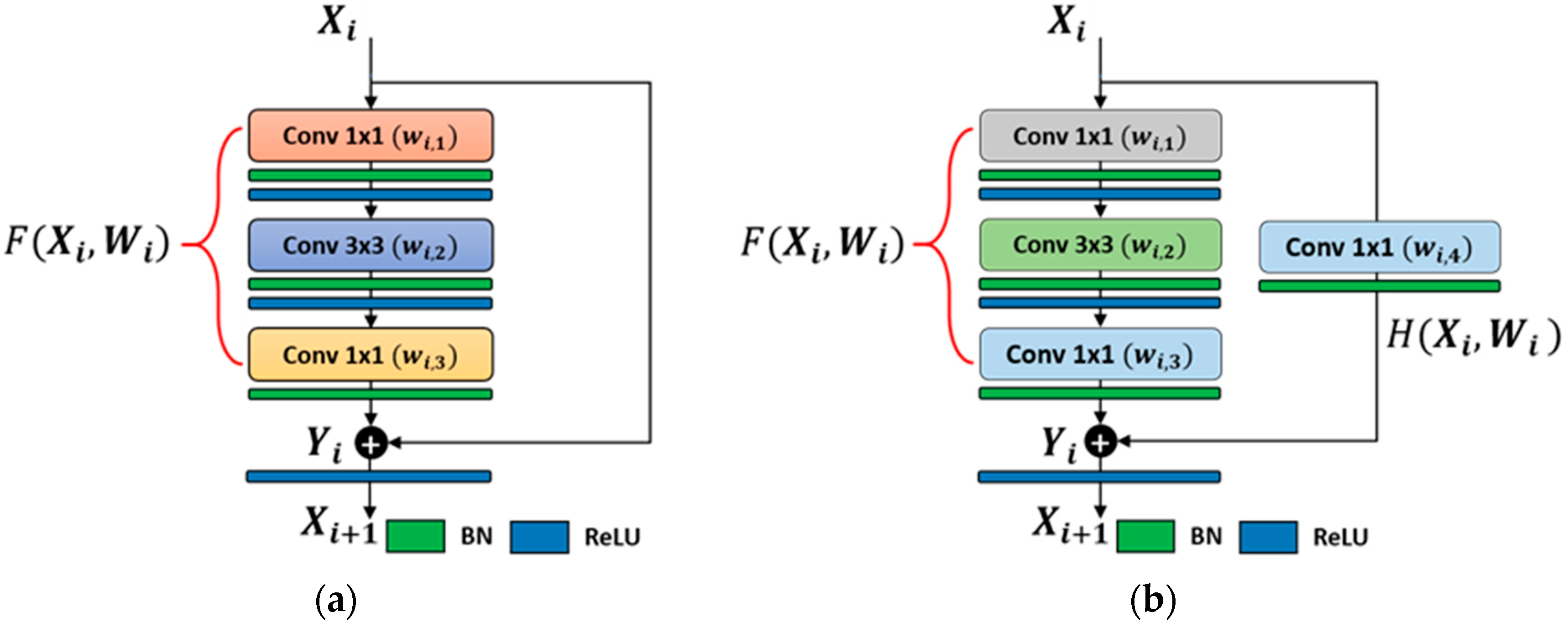
- In our proposed medical image classification and retrieval framework, we modified the conventional ResNet50 [42] CNN model by replacing its last 7 × 7 average pooling layer with a 7 × 7 × 2048 convolutional layer. Finally, the number of nodes in the last fully connected (FC) layer is also adjusted according to the number of classes in our dataset.
- -
- We deeply analyze the characteristics of various CNNs for multiclass medical images, and then check how a specific CNN structure can influence the classification performance of multiclass medical images.
- -
- We compare the performance of state-of-the-art CNN models, not only through fine-tuning and tuning from scratch but also against different handcrafted approaches. Our analysis is more detailed, in contrast to previous studies [10,28], which provided only a limited performance comparison for a small number of databases.
- -
- We analyze the performance of a CNN model based on feature selection from the different layers of the network.
- -
- We have made our trained model and image indices of experimental images publicly available through [43], so that other researchers can evaluate and compare its performance.
4. Proposed Method
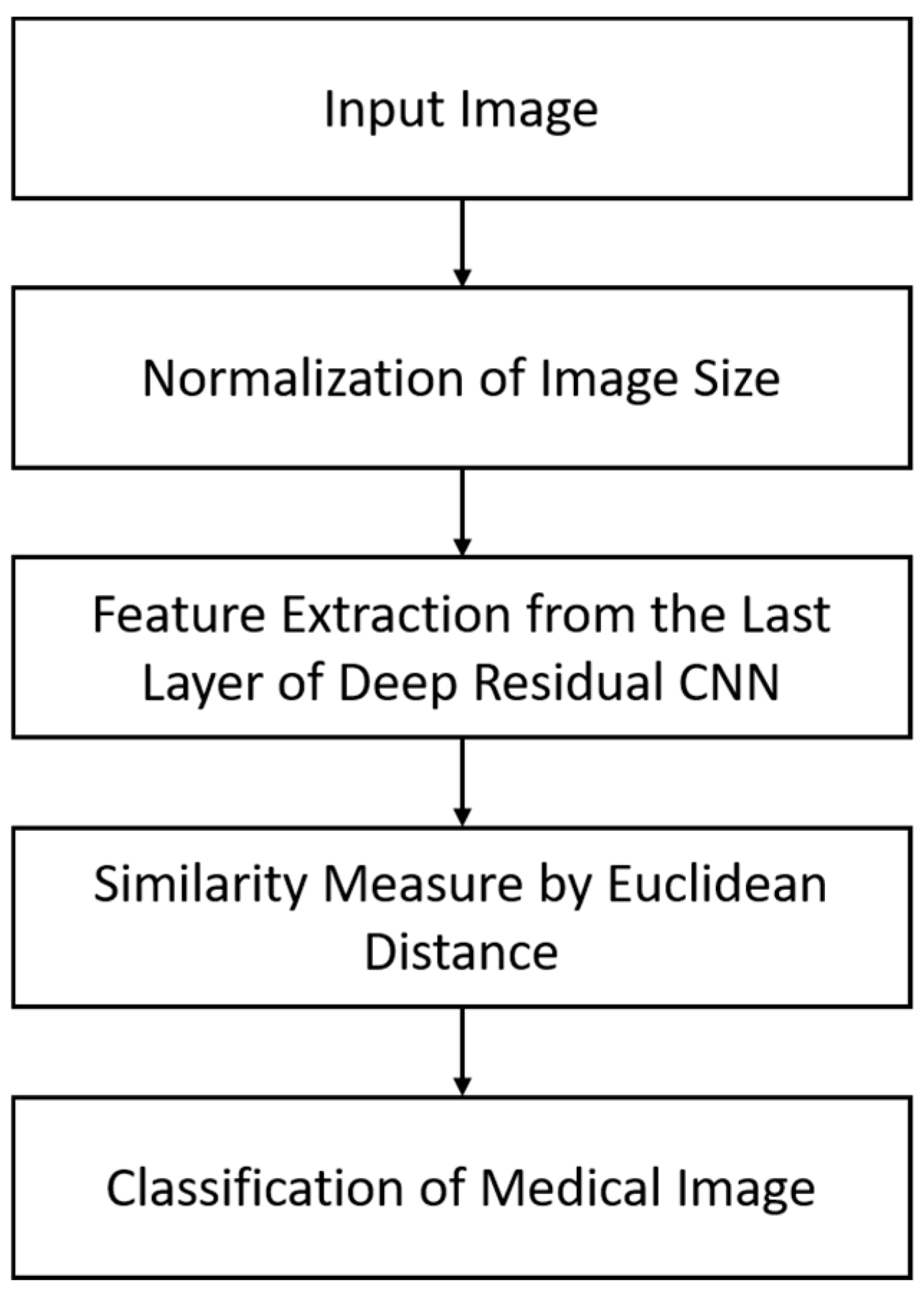
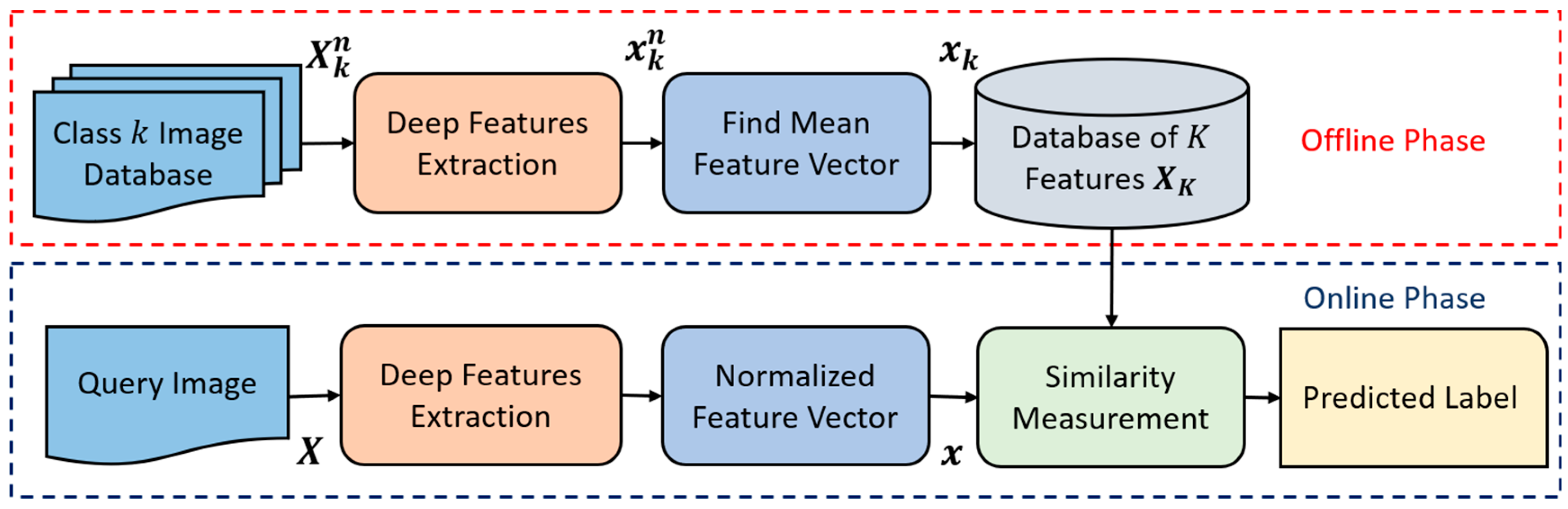
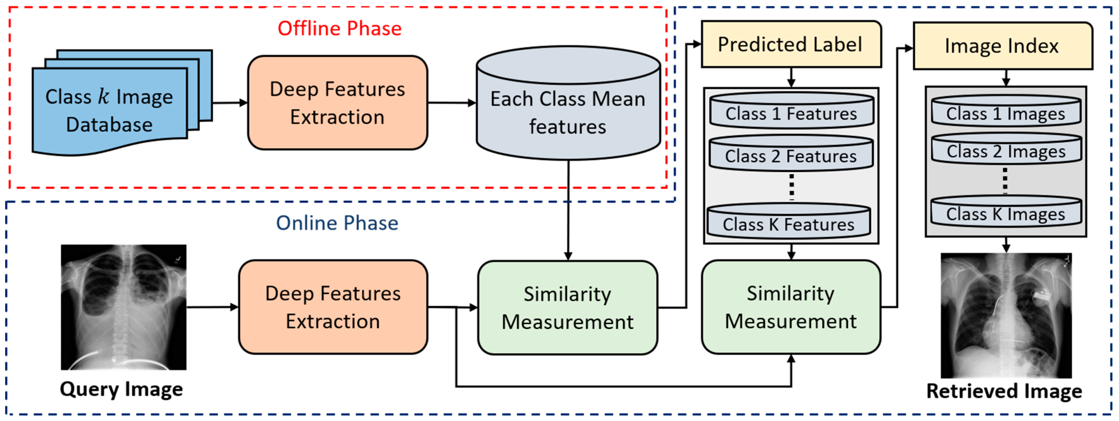
4.1. An Overview of the Proposed Approach
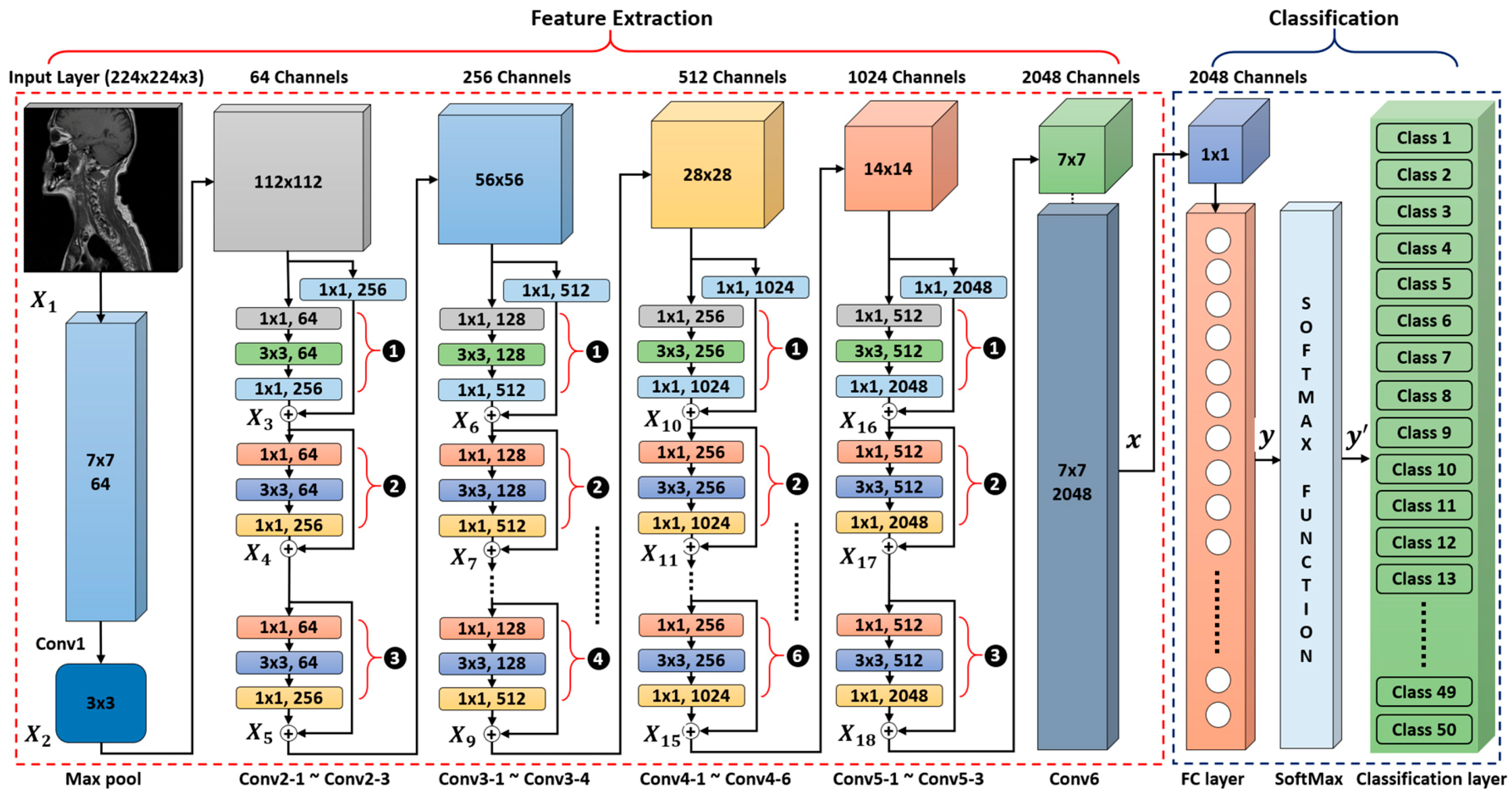
4.2. The Structure of our Modified Deep Residual CNN
4.2.1. Feature Extraction
4.2.2. Classification
5. Experimental Setup and Performance Analysis
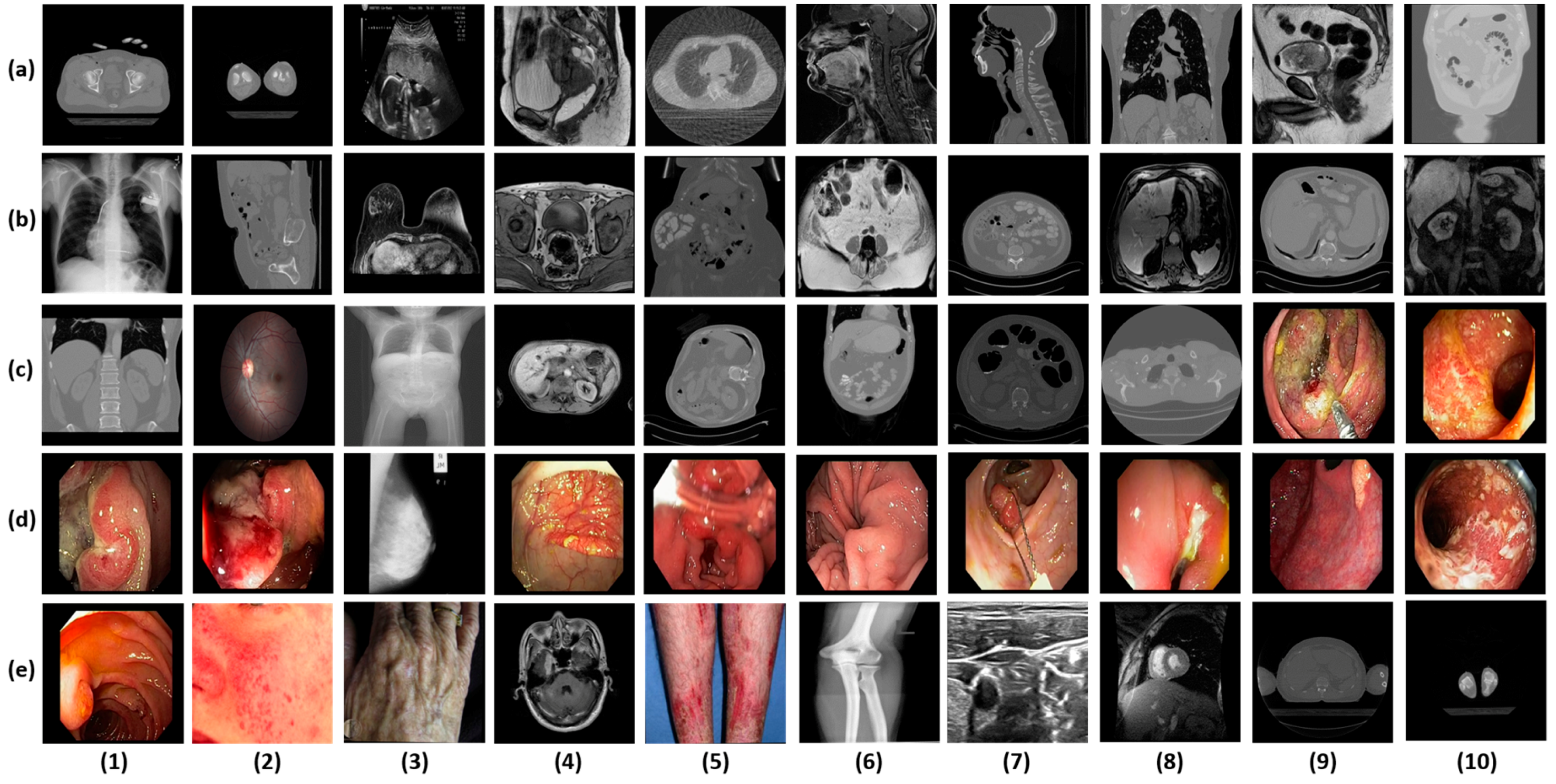
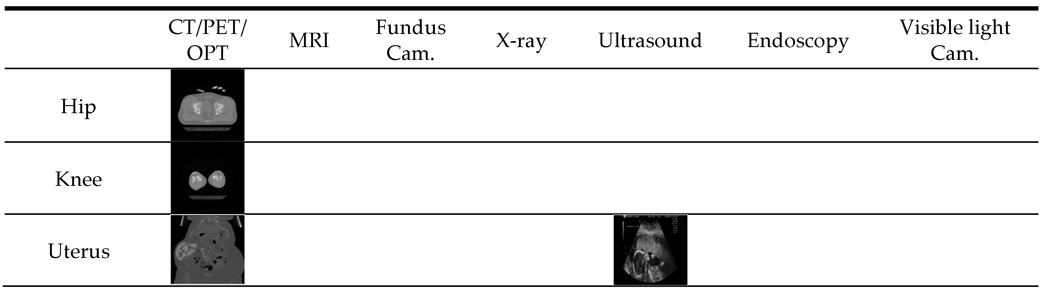
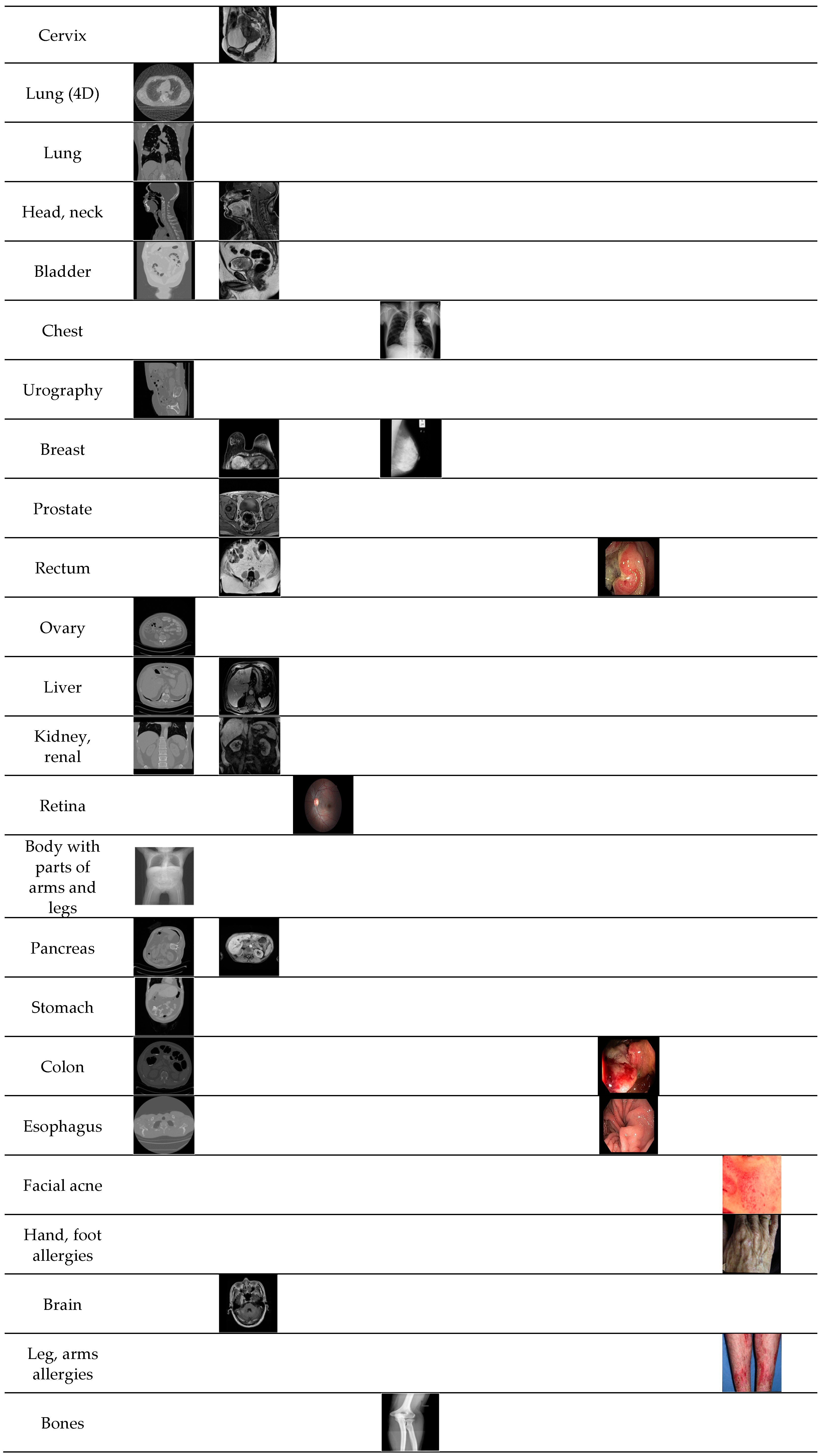
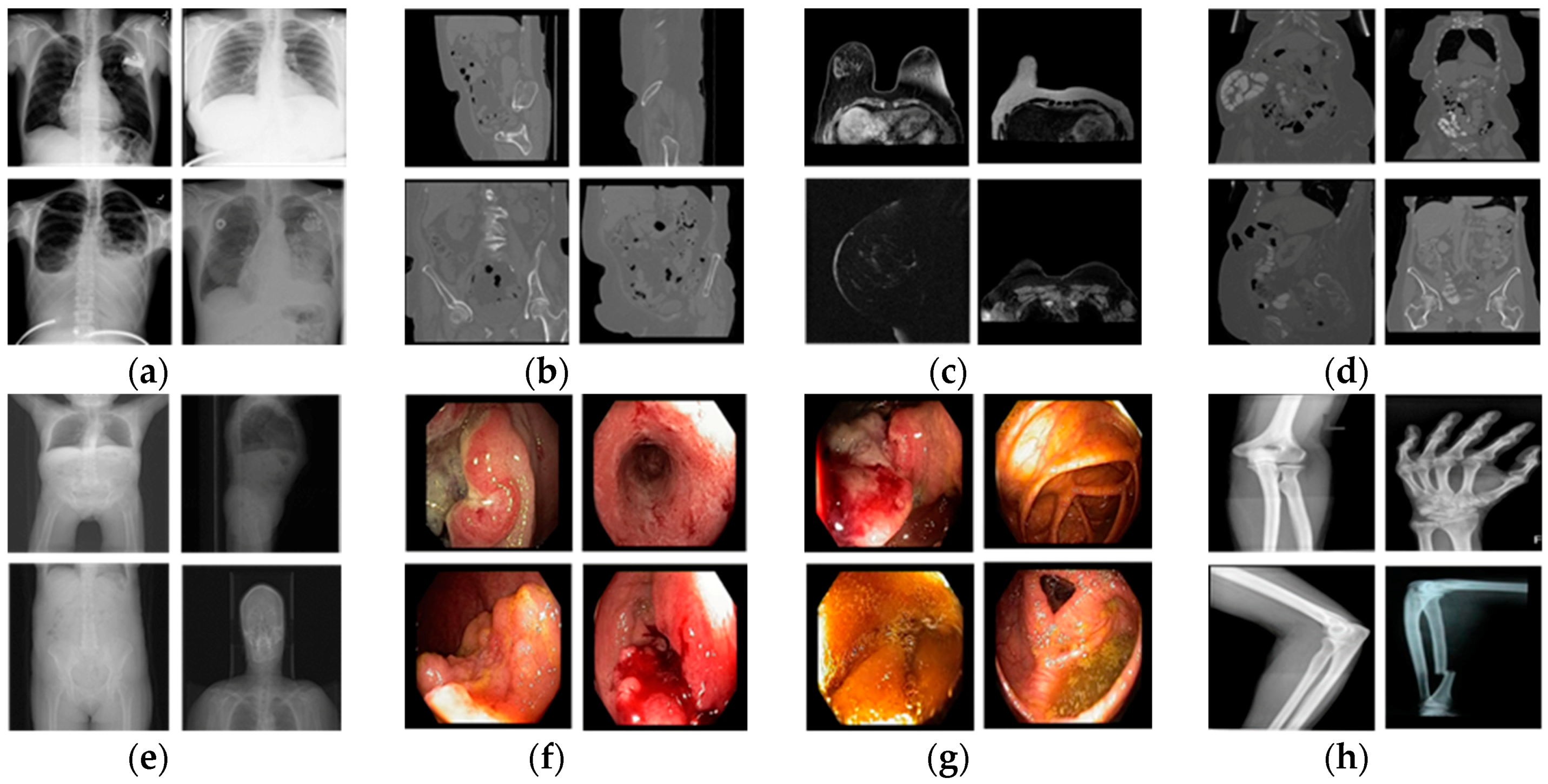
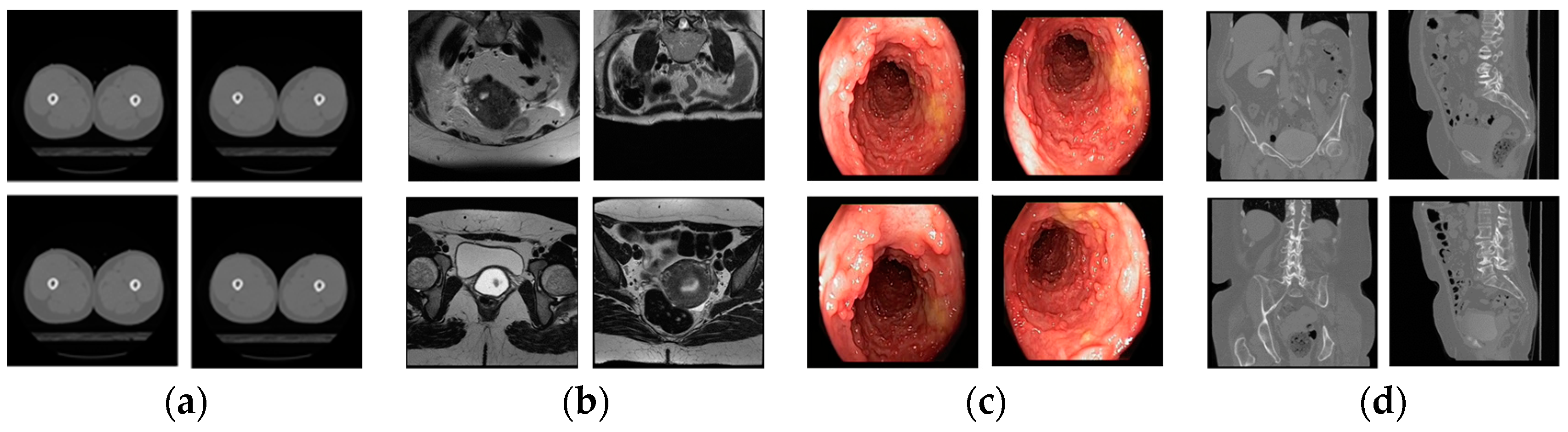
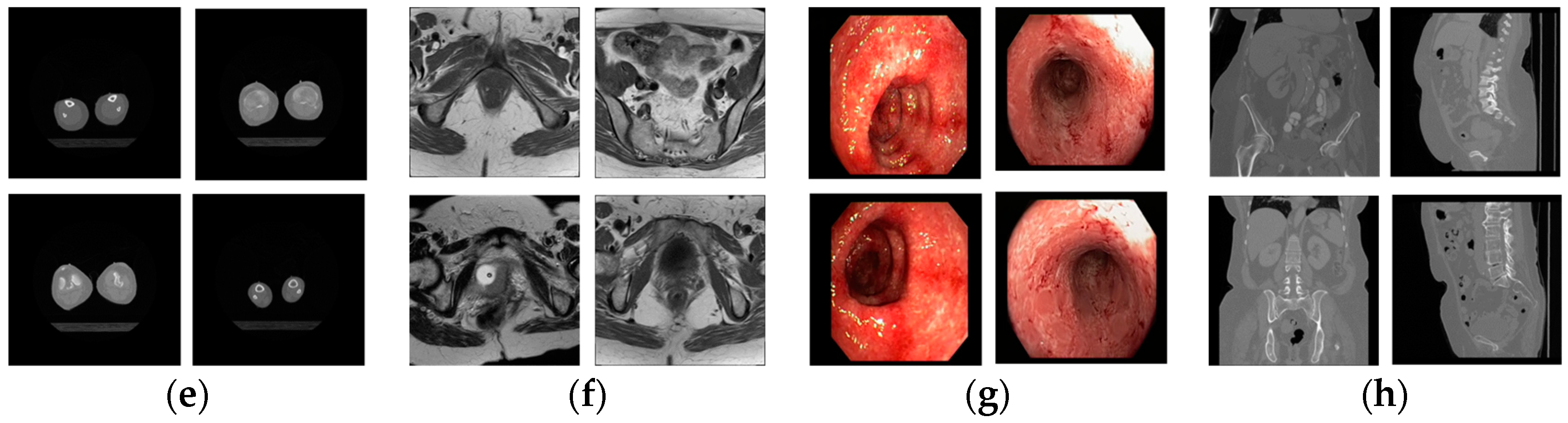
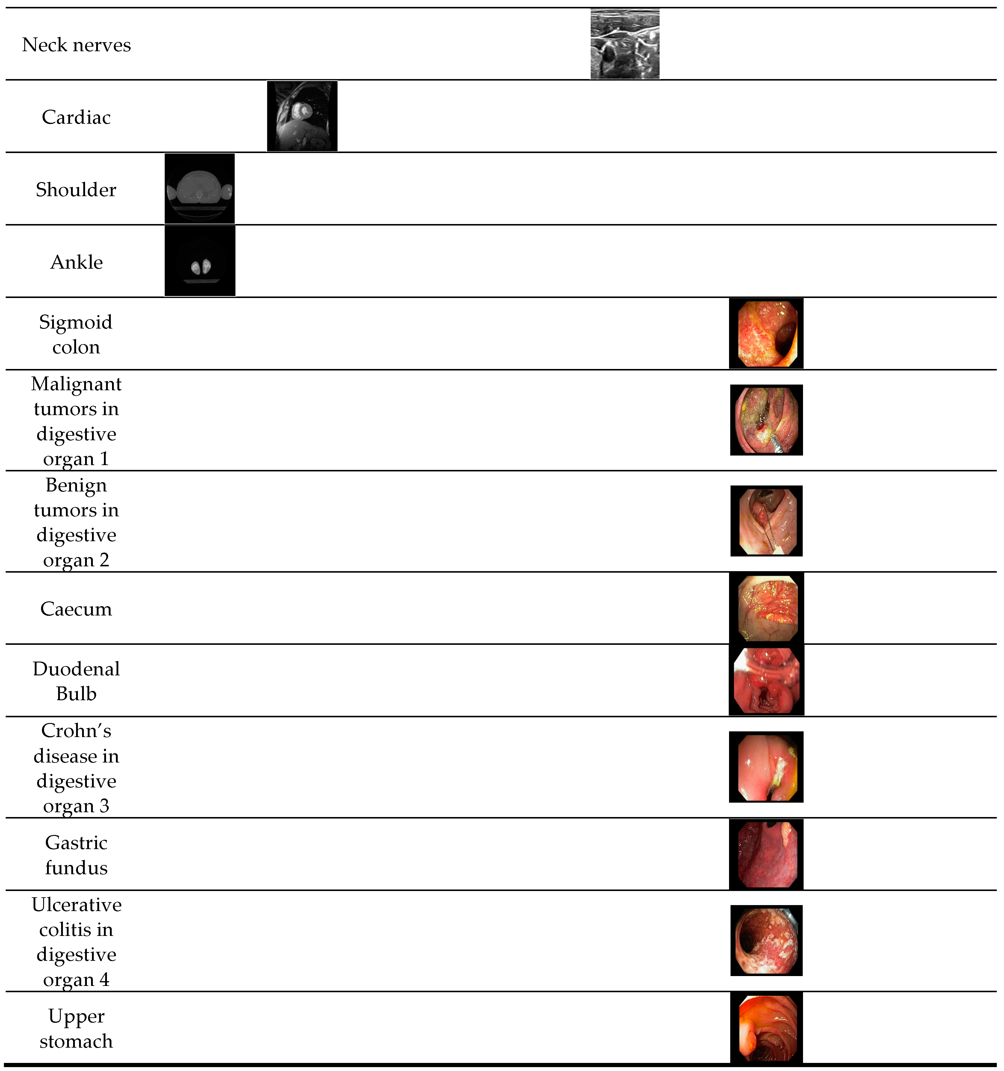
5.1. Dataset and Experimental Protocol
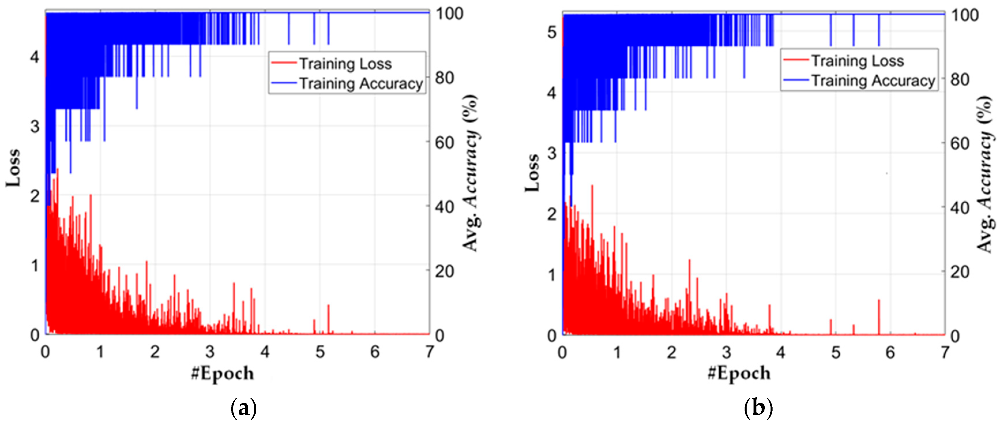
5.2. Training of CNN Model
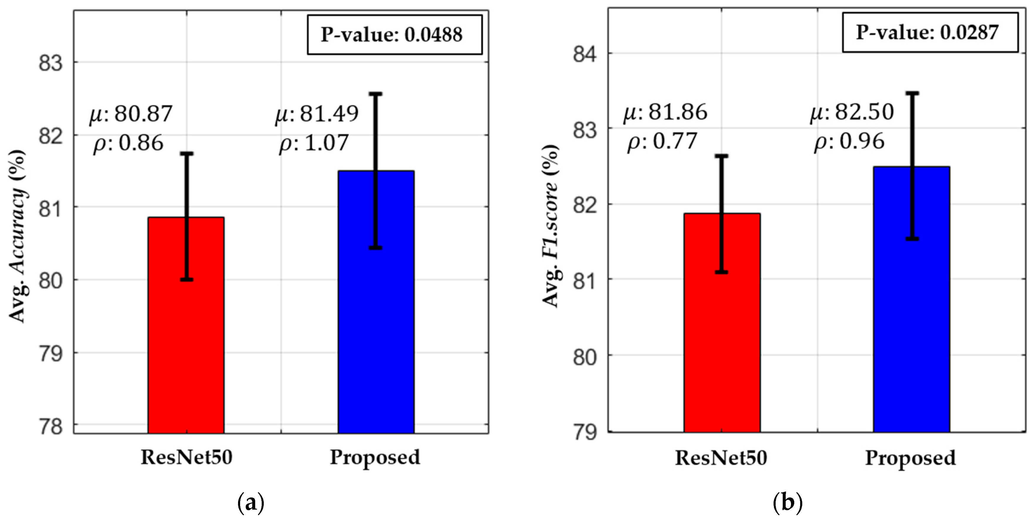
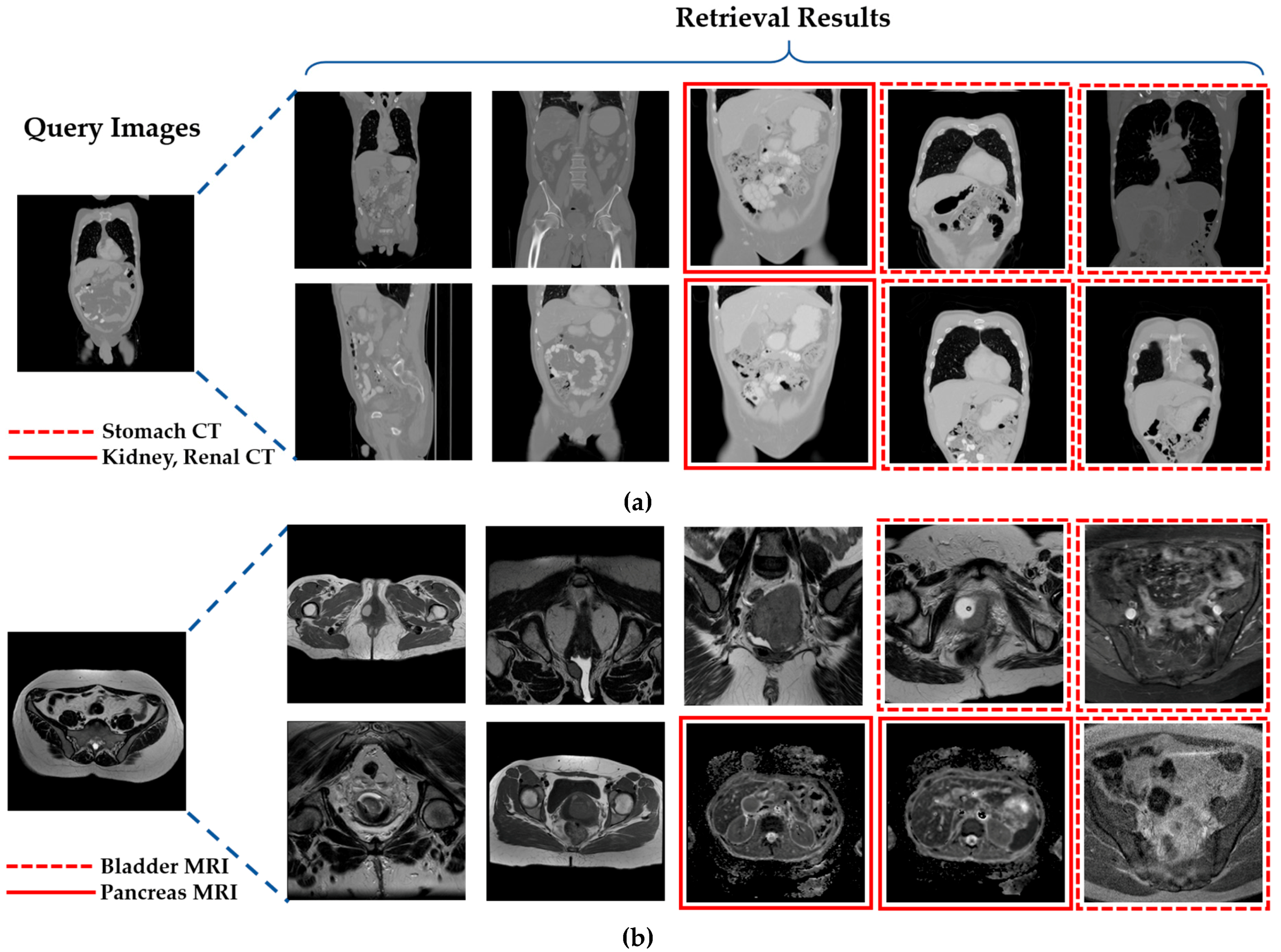
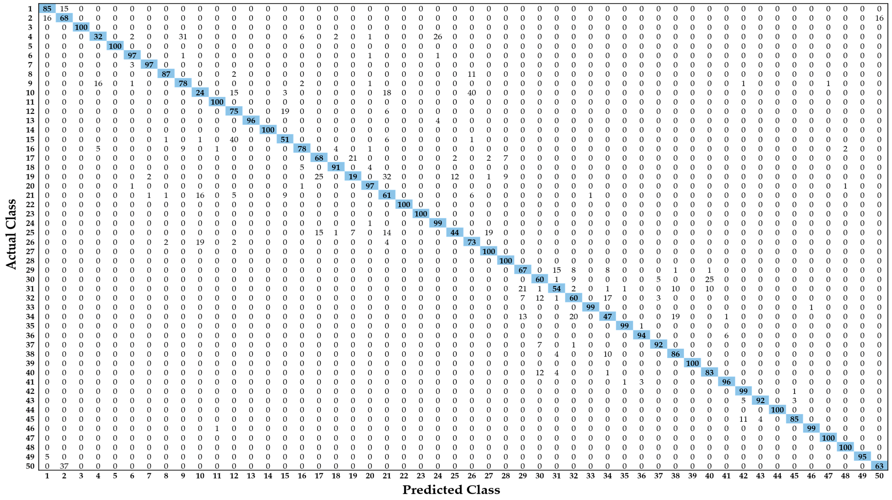
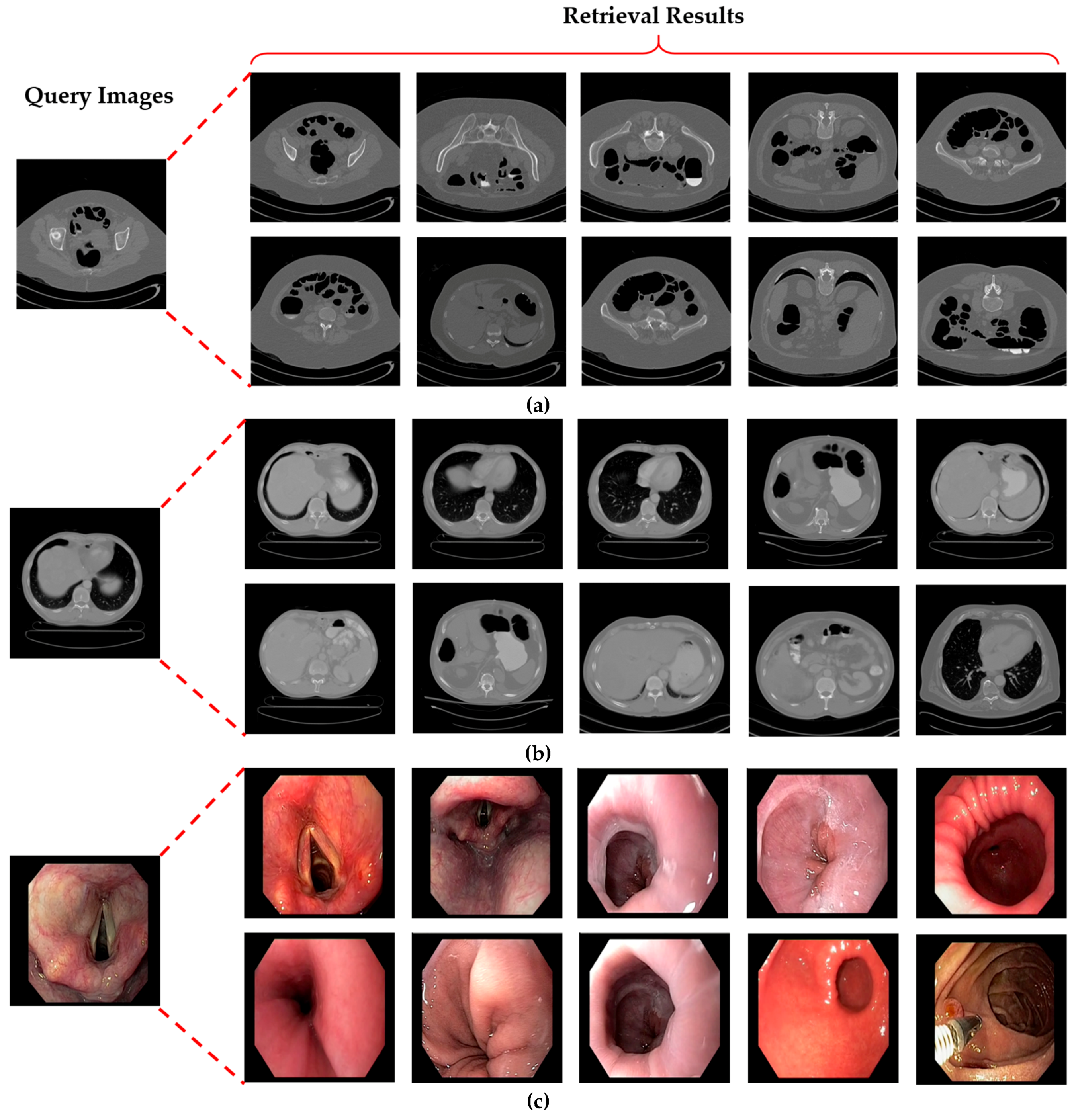
5.3. Testing and Performance Analysis
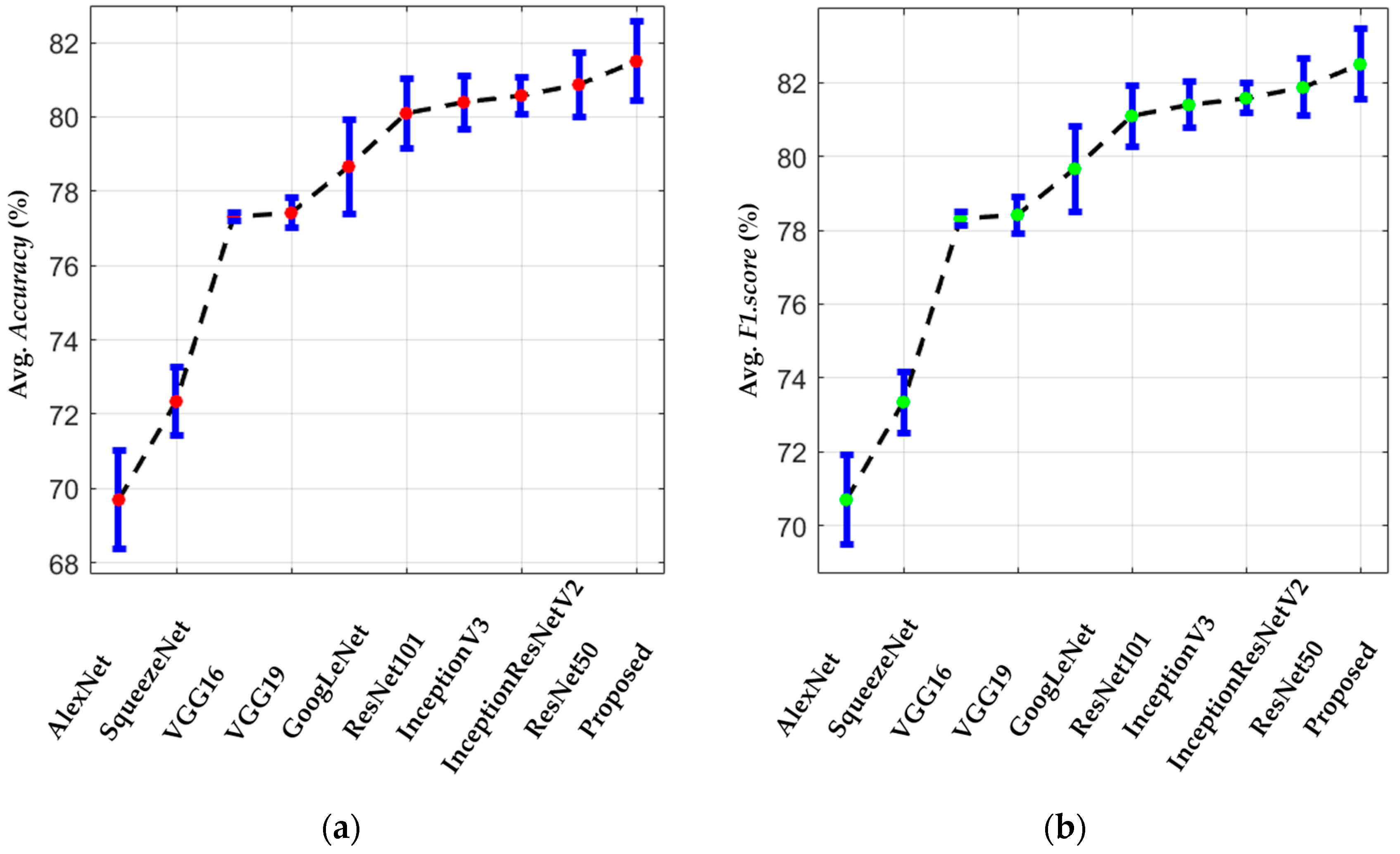
5.3.1. Comparisons of Classification Accuracies by Proposed Modified Residual CNN with Various CNN Models
5.3.2. Comparisons of Classification Accuracies according to the Features from Different Layers
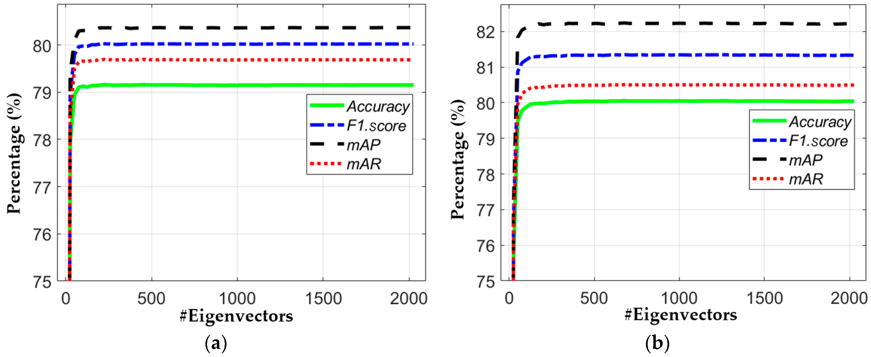
5.3.3. Comparisons of Classification Accuracies with or without Principal Component Analysis
5.3.4. Performance Comparison with Handcrafted Feature-Based Methods
5.3.5. Closed-World vs. Open-World vs. Mixed-World Configurations
6. Discussion
7. Conclusions
Author Contributions
Acknowledgments
Conflicts of Interest
References
- Cheng, C.-H.; Liu, W.-X. Identifying degenerative brain disease using rough set classifier based on wavelet packet method. J. Clin. Med. 2018, 7, 124. [Google Scholar] [CrossRef] [PubMed]
- Purcaru, M.A.P.; Repanovici, A.; Nedeloiu, T. Non-invasive assessment method using thoracic-abdominal profile image acquisition and mathematical modeling with Bezier curves. J. Clin. Med. 2019, 8, 65. [Google Scholar] [CrossRef]
- Tang, J.; Again, S.; Thompson, I. Guest editorial: Computer-aided detection or diagnosis (CAD) systems. IEEE Syst. J. 2014, 8, 907–909. [Google Scholar] [CrossRef]
- Miranda, E.; Aryuni, M.; Irwansyah, E. A survey of medical image classification techniques. In Proceedings of the IEEE International Conference on Information Management and Technology, Bandung, Indonesia, 16–18 November 2016; pp. 56–61. [Google Scholar]
- Wan, J.; Wang, D.; Hoi, S.C.H.; Wu, P.; Zhu, J.; Zhang, Y.; Li, J. Deep learning for content-based image retrieval: A comprehensive study. In Proceedings of the 22nd ACM International Conference on Multimedia, Orlando, FL, USA, 3–7 November 2014; pp. 157–166. [Google Scholar]
- Bengio, Y.; Courville, A.; Vincent, P. Unsupervised feature learning and deep learning: A review and new perspectives. arXiv 2012, arXiv:1206.5538v1. [Google Scholar]
- Yu, D.; Deng, L. Deep learning and its applications to signal and information processing. IEEE Signal Process. Mag. 2011, 28, 145–154. [Google Scholar] [CrossRef]
- Moccia, S.; De Momi, E.; El Hadji, S.; Mattos, L.S. Blood vessel segmentation algorithms—Review of methods, datasets and evaluation metrics. Comput. Meth. Programs Biomed. 2018, 158, 71–91. [Google Scholar] [CrossRef]
- Litjens, G.; Kooi, T.; Bejnordi, B.E.; Setio, A.A.A.; Ciompi, F.; Ghafoorian, M.; van der Laak, J.A.W.M.; van Ginneken, B.; Sánchez, C.I. A survey on deep learning in medical image analysis. Med. Image Anal. 2017, 42, 60–88. [Google Scholar] [CrossRef] [PubMed]
- Tajbakhsh, N.; Shin, J.Y.; Gurudu, S.R.; Hurst, R.T.; Kendall, C.B.; Gotway, M.B.; Liang, J. Convolutional neural networks for medical image analysis: Full training or fine tuning? IEEE Trans. Med. Imaging 2016, 35, 1299–1312. [Google Scholar] [CrossRef]
- Choplin, R.H.; Boehme, J.M., II; Maynard, C.D. Picture archiving and communication systems: An overview. Radiographics 1992, 12, 127–129. [Google Scholar] [CrossRef] [PubMed]
- Graham, R.N.J.; Perriss, R.W.; Scarsbrook, A.F. DICOM demystified: A review of digital file formats and their use in radiological practice. Clin. Radiol. 2005, 60, 1133–1140. [Google Scholar] [CrossRef]
- Avni, U.; Greenspan, H.; Konen, E.; Sharon, M.; Goldberger, J. X-ray categorization and retrieval on the organ and pathology level, using patch-based visual words. IEEE Trans. Med. Imaging 2011, 30, 733–746. [Google Scholar] [CrossRef] [PubMed]
- Orphanoudakis, S.C.; Chronaki, C.; Kostomanolakis, S. I2C: A system for the indexing, storage, and retrieval of medical images by content. Med. Inform. 1994, 19, 109–122. [Google Scholar] [CrossRef]
- Chu, W.W.; Hsu, C.-C.; Cardenas, A.F.; Taira, R.K. Knowledge-based image retrieval with spatial and temporal constructs. IEEE Trans. Knowl. Data Eng. 1998, 10, 872–888. [Google Scholar] [CrossRef]
- El-Kwae, E.A.; Xu, H.; Kabuka, M.R. Content-based retrieval in picture archiving and communication systems. J. Digit. Imaging 2000, 13, 70–81. [Google Scholar] [CrossRef] [PubMed]
- Muller, H.; Rosset, A.; Garcia, A.; Vallee, J.-P.; Geissbuhler, A. Benefits of content-based visual data access in radiology. Radiographics 2005, 25, 849–858. [Google Scholar] [CrossRef]
- Rahman, M.M.; Bhattacharya, P.; Desai, B.C. A framework for medical image retrieval using machine learning and statistical similarity matching techniques with relevance feedback. IEEE Trans. Inf. Technol. Biomed. 2007, 11, 58–69. [Google Scholar] [CrossRef]
- Rahman, M.M.; Bhattacharya, P.; Desai, B.C. A unified image retrieval framework on local visual and semantic concept-based feature spaces. J. Vis. Commun. Image Represent. 2009, 20, 450–462. [Google Scholar] [CrossRef]
- Rahman, M.M.; You, D.; Simpson, M.S.; Antani, S.K.; Demner-Fushman, D.; Thoma, G.R. Multimodal biomedical image retrieval using hierarchical classification and modality fusion. Int. J. Multimed. Inf. Retr. 2013, 2, 159–173. [Google Scholar] [CrossRef]
- Sudhakar, M.S.; Bagan, K.B. An effective biomedical image retrieval framework in a fuzzy feature space employing phase congruency and GeoSOM. Appl. Soft Comput. 2014, 22, 492–503. [Google Scholar] [CrossRef]
- Jyothi, B.; MadhaveeLatha, Y.; Mohan, P.G.K. An effective multiple visual features for content based medical image retrieval. In Proceedings of the IEEE 9th International Conference on Intelligent Systems and Control, Coimbatore, India, 9–10 January 2015; pp. 1–5. [Google Scholar]
- Ramamurthy, B.; Chandran, K.R. CBMIR: Content based medical image retrieval using multilevel hybrid approach. Int. J. Comput. Commun. Control 2015, 10, 382–389. [Google Scholar] [CrossRef]
- Bedo, M.V.N.; dos Santos, D.P.; Ponciano-Silva, M.; de Azevedo-Marques, P.M.; de Carvalho, A.P.D.L.F.; Traina, C., Jr. Endowing a content-based medical image retrieval system with perceptual similarity using ensemble strategy. J. Digit. Imaging 2016, 29, 22–37. [Google Scholar] [CrossRef]
- Malviya, N.; Choudhary, N.; Jain, K. Content based medical image retrieval and clustering based segmentation to diagnose lung cancer. Adv. Comput. Sci. Technol. 2017, 10, 1577–1594. [Google Scholar]
- Kumar, M.; Singh, K.M. Content based medical image retrieval system (CBMIRS) to diagnose hepatobiliary images. In Proceedings of the International Conference on Next Generation Computing Technologies, Dehradun, India, 30–31 October 2017; pp. 663–676. [Google Scholar]
- Kumar, K.K.; Gopal, T.V. A novel approach to self order feature reweighting in CBIR to reduce Semantic gap using relevance feedback. In Proceedings of the IEEE International Conference on Circuit, Power and Computing Technologies, Nagercoil, India, 20–21 March 2014; pp. 1437–1442. [Google Scholar]
- Qayyum, A.; Anwar, S.M.; Awais, M.; Majid, M. Medical image retrieval using deep convolutional neural network. Neurocomputing 2017, 266, 8–20. [Google Scholar] [CrossRef]
- Chowdhury, M.; Bulò, S.R.; Moreno, R.; Kundu, M.K.; Smedby, Ö. An efficient radiographic image retrieval system using convolutional neural network. In Proceedings of the IEEE 23rd International Conference on Patteren Recognition, Cancun, Mexico, 4–8 December 2016; pp. 3134–3139. [Google Scholar]
- Anthimopoulos, M.; Christodoulidis, S.; Ebner, L.; Christe, A.; Mougiakakou, S. Lung pattern classification for interstitial lung diseases using a deep convolutional neural network. IEEE Trans. Med. Imaging 2016, 35, 1207–1216. [Google Scholar] [CrossRef]
- Van Tulder, G.; de Bruijne, M. Combining generative and discriminative representation learning for lung CT analysis with convolutional restricted Boltzmann machines. IEEE Trans. Med. Imaging 2016, 35, 1262–1272. [Google Scholar] [CrossRef]
- Ciompi, F.; de Hoop, B.; van Riel, S.J.; Chung, K.; Scholten, E.T.; Oudkerk, M.; de Jong, P.A.; Prokop, M.; van Ginneken, B. Automatic classification of pulmonary peri-fissural nodules in computed tomography using an ensemble of 2D views and a convolutional neural network out-of-the-box. Med. Image Anal. 2015, 26, 195–202. [Google Scholar] [CrossRef]
- Yan, Z.; Zhan, Y.; Peng, Z.; Liao, S.; Shinagawa, Y.; Zhang, S.; Metaxas, D.N.; Zhou, X.S. Multi-instance deep learning: Discover discriminative local anatomies for bodypart recognition. IEEE Trans. Med. Imaging 2016, 35, 1332–1343. [Google Scholar] [CrossRef] [PubMed]
- Dou, Q.; Chen, H.; Yu, L.; Zhao, L.; Qin, J.; Wang, D.; Mok, V.C.; Shi, L.; Heng, P.-A. Automatic detection of cerebral microbleeds from MR images via 3D convolutional neural networks. IEEE Trans. Med. Imaging 2016, 35, 1182–1195. [Google Scholar] [CrossRef]
- Van Grinsven, M.J.J.P.; van Ginneken, B.; Hoyng, C.B.; Theelen, T.; Sánchez, C.I. Fast convolutional neural network training using selective data sampling: Application to hemorrhage detection in color fundus images. IEEE Trans. Med. Imaging 2016, 35, 1273–1284. [Google Scholar] [CrossRef] [PubMed]
- Setio, A.A.A.; Ciompi, F.; Litjens, G.; Gerke, P.; Jacobs, C.; van Riel, S.J.; Wille, M.M.W.; Naqibullah, M.; Sánchez, C.I.; van Ginneken, B. Pulmonary nodule detection in CT images: False positive reduction using multi-view convolutional networks. IEEE Trans. Med. Imaging 2016, 35, 1160–1169. [Google Scholar] [CrossRef]
- Shin, H.-C.; Roth, H.R.; Gao, M.; Lu, L.; Xu, Z.; Nogues, I.; Yao, J.; Mollura, D.; Summers, R.M. Deep convolutional neural networks for computer-aided detection: CNN architectures, dataset characteristics and transfer learning. IEEE Trans. Med. Imaging 2016, 35, 1285–1298. [Google Scholar] [CrossRef]
- Jiang, F.; Jiang, Y.; Zhi, H.; Dong, Y.; Li, H.; Ma, S.; Wang, Y.; Dong, Q.; Shen, H.; Wang, Y. Artificial intelligence in healthcare: Past, present and future. Stroke Vasc. Neurol. 2017, 2, 230–243. [Google Scholar] [CrossRef]
- Gupta, M.R.; Bengio, S.; Weston, J. Training highly multiclass classifiers. J. Mach. Learn. Res. 2014, 15, 1461–1492. [Google Scholar]
- Brucker, F.; Benites, F.; Sapozhnikova, E. Multi-label classification and extracting predicted class hierarchies. Pattern Recognit. 2011, 44, 724–738. [Google Scholar] [CrossRef]
- Silva-Palacios, D.; Ferri, C.; Ramirez-Quintana, M.J. Improving performance of multiclass classification by inducing class hierarchies. In Proceedings of the International Conference on Computational Science, Zurich, Switzerland, 12–14 June 2017; pp. 1692–1701. [Google Scholar]
- He, K.; Zhang, X.; Ren, S.; Sun, J. Deep residual learning for image recognition. In Proceedings of the IEEE Conference on Computer Vision and Pattern Recognition, Las Vegas, NV, USA, 26 June–1 July 2016; pp. 770–778. [Google Scholar]
- Dongguk CNN Model and Image Indices of Open Databases for CBMIR. Available online: http://dm.dgu.edu/link.html (accessed on 15 February 2019).
- He, K.; Zhang, X.; Ren, S.; Sun, J. Identity mappings in deep residual networks. In Proceedings of the European Conference on Computer Vision, Amsterdam, The Netherlands, 11–14 October 2016; pp. 630–645. [Google Scholar]
- Heaton, J. Artificial Intelligence for Humans; Deep learning and neural networks; Heaton Research Inc.: St. Louis, MO, USA, 2015; Volume 3. [Google Scholar]
- MICCAI Grand Challenges. Available online: https://grand-challenge.org/challenges/ (accessed on 29 March 2019).
- Chest X-rays Database. Available online: https://nihcc.app.box.com/v/ChestXray-NIHCC (accessed on 1 February 2019).
- Decenciere, E.; Zhang, X.; Cazuguel, G.; Lay, B.; Cochener, B.; Trone, C.; Gain, P.; Ordonez-Varela, J.-R.; Massin, P.; Erginay, A.; et al. Feedback on a publicly distributed image database: The Messidor database. Image Anal. Stereol. 2014, 33, 231–234. [Google Scholar] [CrossRef]
- Suckling, J.; Parker, J.; Dance, D.R.; Astley, S.; Hutt, I.; Boggis, C.; Ricketts, I.; Stamatakis, E.; Cerneaz, N.; Kok, S.L.; et al. The mammographic image analysis society digital mammogram database. In Proceedings of the 2nd International Workshop on Digital Mammography, York, UK, 10–12 July 1994; pp. 375–378. [Google Scholar]
- Brain Tumor Database. Available online: https://figshare.com/articles/brain_tumor_dataset /1512427 (accessed on 1 February 2019).
- Bones X-rays Database. Available online: https://sites.google.com/site/mianalysis16/ (accessed on 1 February 2019).
- Neck Nerve Structure Database. Available online: https://www.kaggle.com/c/ultrasound-nerve-segmentation/data (accessed on 1 February 2019).
- Radau, P.; Lu, Y.; Connelly, K.; Paul, G.; Dick, A.J.; Wright, G.A. Evaluation Framework for Algorithms Segmenting Short Axis Cardiac MRI. Available online: https://www.midasjournal.org/browse/publication/658 (accessed on 5 April 2019).
- Visible Human Project CT Datasets. Available online: https://mri.radiology.uiowa.edu/visible_human_datasets.html (accessed on 1 February 2019).
- Baby Ultrasound Videos. Available online: https://youtu.be/SrUoXkKoREE (accessed on 1 February 2019).
- Clark, K.; Vendt, B.; Smith, K.; Freymann, J.; Kirby, J.; Koppel, P.; Moore, S.; Phillips, S.; Maffitt, D.; Pringle, M.; et al. The cancer imaging archive (TCIA): Maintaining and operating a public information repository. J. Digit. Imaging 2013, 26, 1045–1057. [Google Scholar] [CrossRef] [PubMed]
- Endoscopy Videos. Available online: http://www.gastrolab.net/ni.htm (accessed on 1 February 2019).
- Skin’s Diseases Database. Available online: https://www.dermnetnz.org/image-licence/#use (accessed on 1 February 2019).
- Wong, S.C.; Gatt, A.; Stamatescu, V.; McDonnell, M.D. Understanding data augmentation for classification: When to warp? In Proceedings of the IEEE International Conference on Digital Image Computing: Techniques and Applications, Gold Coast, Australia, 30 November–2 December 2016; pp. 1–6. [Google Scholar]
- Intel® Core™ i7-3770K Processor. Available online: https://ark.intel.com/content/www/us/en/ark/products/65523/intel-core-i7-3770k-processor-8m-cache-up-to-3-90-ghz.html (accessed on 1 February 2019).
- GeForce GTX 1070. Available online: https://www.geforce.com/hardware/desktop-gpus/geforce-gtx-1070/specifications (accessed on 1 February 2019).
- MATLAB R2018b. Available online: https://ch.mathworks.com/products/new_products/latest_features.html (accessed on 1 February 2019).
- Bottou, L. Stochastic gradient descent tricks. In Neural Networks: Tricks of the Trade; Springer: Berlin, Germany, 2012; pp. 421–436. [Google Scholar]
- Training Options. Available online: http://kr.mathworks.com/help/nnet/ref/trainingoptions.html (accessed on 1 February 2019).
- Hossin, M.; Sulaiman, M.N. A review on evaluation metrics for data classification evaluations. Int. J. Data Min. Knowl. Manag. Process 2015, 5, 1–11. [Google Scholar]
- Takiyama, H.; Ozawa, T.; Ishihara, S.; Fujishiro, M.; Shichijo, S.; Nomura, S.; Miura, M.; Tada, T. Automatic anatomical classification of esophagogastroduodenoscopy images using deep convolutional neural networks. Sci. Rep. 2018, 8, 7497. [Google Scholar] [CrossRef] [PubMed]
- Iandola, F.N.; Han, S.; Moskewicz, M.W.; Ashraf, K.; Dally, W.J.; Keutzer, K. SqueezeNet: AlexNet-level accuracy with 50x fewer parameters and <0.5 MB model size. arXiv 2016, arXiv:1602.07360v4. [Google Scholar]
- Simonyan, K.; Zisserman, A. Very deep convolutional networks for large-scale image recognition. In Proceedings of the 3rd International Conference on Learning Representations, San Diego, CA, USA, 7–9 May 2015; pp. 1–14. [Google Scholar]
- Szegedy, C.; Liu, W.; Jia, Y.; Sermanet, P.; Reed, S.; Anguelov, D.; Erhan, D.; Vanhoucke, V.; Rabinovich, A. Going deeper with convolutions. In Proceedings of the IEEE Conference Computer Vision and Pattern Recognition, Boston, MA, USA, 7–12 June 2015; pp. 1–9. [Google Scholar]
- Szegedy, C.; Vanhoucke, V.; Ioffe, S.; Shlens, J.; Wojna, Z. Rethinking the inception architecture for computer vision. In Proceedings of the IEEE Conference on Computer Vision and Pattern Recognition, Las Vegas, NV, USA, 27–30 June 2016; pp. 2818–2826. [Google Scholar]
- Szegedy, C.; Ioffe, S.; Vanhoucke, V.; Alemi, A.A. Inception-v4, Inception-ResNet and the impact of residual connections on learning. In Proceedings of the 31st AAAI Conference on Artificial Intelligence, San Francisco, CA, USA, 4–9 February 2017; pp. 4278–4284. [Google Scholar]
- Deng, J.; Dong, W.; Socher, R.; Li, L.-J.; Li, K.; Fei-Fei, L. ImageNet: A large-scale hierarchical image database. In Proceedings of the IEEE Conference on Computer Vision and Pattern Recognition, Miami, FL, USA, 20–25 June 2009; pp. 248–255. [Google Scholar]
- Raychaudhuri, S. Introduction to Monte Carlo simulation. In Proceedings of the IEEE Winter Simulation Conference, Miami, FL, USA, 7–10 December 2008; pp. 91–100. [Google Scholar]
- Student’s t-Test. Available online: https://en.wikipedia.org/wiki/Student%27s_t-test (accessed on 1 February 2019).
- Ilin, A.; Raiko, T. Practical approaches to principal component analysis in the presence of missing values. J. Mach. Learn. Res. 2010, 11, 1957–2000. [Google Scholar]
- Subrahmanyam, M.; Maheshwari, R.P.; Balasubramanian, R. Local maximum edge binary patterns: A new descriptor for image retrieval and object tracking. Signal Process. 2012, 92, 1467–1479. [Google Scholar] [CrossRef]
- Velmurugan, K.; Baboo, L.D.S.S. Image retrieval using Harris corners and histogram of oriented gradients. Int. J. Comput. Appl. 2011, 24, 6–10. [Google Scholar]


| Imaging Modalities | Method | Number of Classes | Strength | Weakness | |
|---|---|---|---|---|---|
| Single modality | CT | Pre-trained CNN [32] | 2 | Classification performance reaches that of a human observer | Classify only lung cancer CT scan images rather than multiclass images |
| X-ray | CNN + edge histogram features are selected [29] | 31 | High classification performance | Limited dataset (i.e., 1550 images) related to 31 classes (i.e., 50 images in each class) and only 10 images per class are selected for calculating system performance | |
| CT | Deep CNN model [30] | 7 | High CAD sensitivity performance with less computation time | Only classify infected and non-infected lung CT scans | |
| CT | Two-stage multiple instance CNN [33] | 12 | High classification accuracy | Limited dataset and number of classes | |
| MRI | 3D CNN-based discrimination model [34] | 2 | High sensitivity | Only classify infected and non-infected brain MRI scans (only 2 classes) | |
| Fundus camera | CNN + selective sampling (SeS) [35] | 2 | High average classification accuracy | Uses the reference guide from a single expert | |
| CT | Restricted Boltzmann machine (RBM) [31] | 5 | High average classification accuracy | Suitable for smaller representations learning with smaller filters or hidden nodes | |
| CT | Multiview convolutional network (ConvNets) [36] | 2 | False positive error is reduced | The CAD sensitivity performance should be enhanced | |
| Multiple modalities | CT, MRI, fundus camera, PET, OPT | Content-based medical image retrieval system (CBMIR) by using CNN [28] | 24 | High classification accuracy | - A limited number of experimental images - Performance was measured only by closed-world configuration |
| CT, MRI, fundus camera, PET, OPT, X-ray, ultrasound, endoscopy, visible light camera | Proposed method | 50 | - High classification performance for multiple modalities data. - Number of classes is much larger than that in the previous work | Using deeper CNN requires more training time | |
| Layer Name | Feature Map Size | Number of Filters | Kernel Size | Stride | Number of Padding | Number of Iterations | |
|---|---|---|---|---|---|---|---|
| Image input layer | 224 × 224 × 3 | ||||||
| Conv1 | 112 × 112 × 64 | 64 | 7 × 7 × 3 | 2 | 3 | 1 | |
| Max pool | 56 × 56 × 64 | 1 | 3 × 3 | 2 | 0 | 1 | |
| Conv2 | Conv2-1 (1 × 1 Convolutional Mapping) | 56 × 56 × 64 | 64 | 1 × 1 × 64 | 1 | 0 | 1 |
| 56 × 56 × 64 | 64 | 3 × 3 × 64 | 1 | 1 | |||
| 56 × 56 × 256 | 256 | 1 × 1 × 64 | 1 | 0 | |||
| 56 × 56 × 256 | 256 | 1 × 1 × 64 | 1 | 0 | |||
| Conv2-2–Conv2-3 (Identity Mapping) | 56 × 56 × 64 | 64 | 1 × 1 × 256 | 1 | 0 | 2 | |
| 56 × 56 × 64 | 64 | 3 × 3 × 64 | 1 | 1 | |||
| 56 × 56 × 256 | 256 | 1 × 1 × 64 | 1 | 0 | |||
| Conv3 | Conv3-1 (1 × 1 Convolutional Mapping) | 28 × 28 × 128 | 128 | 1 × 1 × 256 | 2 | 0 | 1 |
| 28 × 28 × 128 | 128 | 3 × 3 × 128 | 1 | 1 | |||
| 28 × 28 × 512 | 512 | 1 × 1 × 128 | 1 | 0 | |||
| 28 × 28 × 512 | 512 | 1 × 1 × 256 | 2 | 0 | |||
| Conv3-2–Conv3-4 (Identity Mapping) | 28 × 28 × 128 | 128 | 1 × 1 × 512 | 1 | 0 | 3 | |
| 28 × 28 × 128 | 128 | 3 × 3 × 128 | 1 | 1 | |||
| 28 × 28 × 512 | 512 | 1 × 1 × 128 | 1 | 0 | |||
| Conv4 | Conv4-1 (1 × 1 Convolutional Mapping) | 14 × 14 × 256 | 256 | 1 × 1 × 512 | 2 | 0 | 1 |
| 14 × 14 × 256 | 256 | 3 × 3 × 256 | 1 | 1 | |||
| 14 × 14 × 1024 | 1024 | 1 × 1 × 256 | 1 | 0 | |||
| 14 × 14 × 1024 | 1024 | 1 × 1 × 512 | 2 | 0 | |||
| Conv4-2–Conv4-6 (Identity Mapping) | 14 × 14 × 256 | 256 | 1 × 1 × 1024 | 1 | 0 | 5 | |
| 14 × 14 × 256 | 256 | 3 × 3 × 256 | 1 | 1 | |||
| 14 × 14 × 1024 | 1024 | 1 × 1 × 256 | 1 | 0 | |||
| Conv5 | Conv5-1 (1 × 1 Convolutional Mapping) | 7 × 7 × 512 | 512 | 1 × 1 × 1024 | 2 | 0 | 1 |
| 7 × 7 × 512 | 512 | 3 × 3 × 512 | 1 | 1 | |||
| 7 × 7 × 2048 | 2048 | 1 × 1 × 512 | 1 | 0 | |||
| 7 × 7 × 2048 | 2048 | 1 × 1 × 1024 | 2 | 0 | |||
| Conv5-2–Conv5-3 (Identity Mapping) | 7 × 7 × 512 | 512 | 1 × 1 × 2048 | 1 | 0 | 2 | |
| 7 × 7 × 512 | 512 | 3 × 3 × 512 | 1 | 1 | |||
| 7 × 7 × 2048 | 2048 | 1 × 1 × 512 | 1 | 0 | |||
| Conv6 | 1 × 1 × 2048 | 2048 | 7 × 7 × 2048 | 1 | 0 | 1 | |
| FC layer | 50 | 1 | |||||
| SoftMax | 50 | 1 | |||||
| Classification layer | 50 | 1 | |||||
| Configurations | Validation | Training | Testing | Total | |
|---|---|---|---|---|---|
| Original | Augmented | ||||
| Closed-world | 1st fold | 22,732 | 2268 | 22,732 | 47,732 |
| 2nd fold | 22,732 | 2268 | 22,732 | 47,732 | |
| Open-world | 1st fold | 21,870 | 3130 | 23,594 | 48,594 |
| 2nd fold | 23,594 | 1406 | 21,870 | 46,870 | |
| Mixed-world | 1st fold | 18,435 | 1565 | 27,029 | 47,029 |
| 2nd fold | 18,435 | 1565 | 27,029 | 47,029 | |
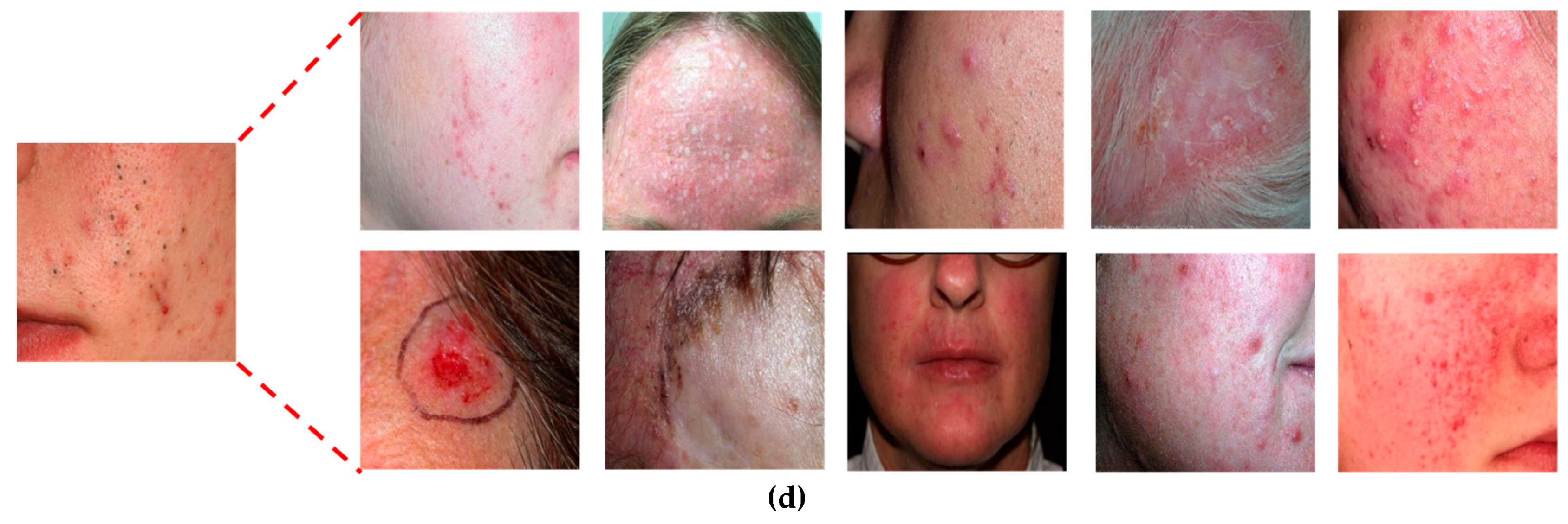
| Caption Detail as in Figure 5 | Class Name | Class Imbalance Details | |||
|---|---|---|---|---|---|
| Original | Augmented | Total | Imbalance Ratio (%) | ||
| d-3 | Breast mammogram | 161 | 339 | 500 | 67.8 |
| e-6 | Bones X-rays | 169 | 331 | 500 | 66.2 |
| e-9 | Shoulder CT | 455 | 45 | 500 | 9 |
| e-10 | Ankle CT | 75 | 425 | 500 | 85 |
| a-1 | Hip CT | 400 | 100 | 500 | 20 |
| a-2 | Knee CT | 175 | 325 | 500 | 65 |
| e-2 | Facial acne | 487 | 13 | 500 | 2.6 |
| e-3 | Hand, foot allergies | 238 | 262 | 500 | 52.4 |
| e-5 | Legs, arms allergies | 72 | 428 | 500 | 85.6 |
| CNN Model | Accuracy | F1.score | mAP | mAR | ||||||||
|---|---|---|---|---|---|---|---|---|---|---|---|---|
| Fold1 | Fold2 | Avg. | Fold1 | Fold2 | Avg. | Fold1 | Fold2 | Avg. | Fold1 | Fold2 | Avg. | |
| AlexNet [28] | 71.01 | 68.41 | 69.71 | 71.43 | 67.84 | 69.63 | 72.42 | 68.21 | 70.31 | 70.47 | 67.47 | 68.97 |
| SqueezeNet [66] | 73.21 | 71.43 | 72.32 | 74.45 | 73.79 | 74.12 | 76.64 | 75.50 | 76.07 | 72.37 | 72.16 | 72.27 |
| VGG16 [68] | 77.38 | 77.33 | 77.36 | 78.01 | 78.44 | 78.22 | 78.83 | 79.29 | 79.06 | 77.21 | 77.60 | 77.41 |
| VGG19 [68] | 77.10 | 77.82 | 77.46 | 77.98 | 78.53 | 78.25 | 79.01 | 79.14 | 79.08 | 76.97 | 77.92 | 77.45 |
| GoogLeNet [66,69] | 79.94 | 77.37 | 78.66 | 80.90 | 78.11 | 79.51 | 82.39 | 78.08 | 80.23 | 79.47 | 78.15 | 78.81 |
| ResNet101 [42] | 81.08 | 79.16 | 80.12 | 81.81 | 80.54 | 81.17 | 82.85 | 80.87 | 81.86 | 80.79 | 80.20 | 80.50 |
| ResNet50 [42] | 81.29 | 79.54 | 80.42 | 82.18 | 80.65 | 81.41 | 83.29 | 80.74 | 82.01 | 81.09 | 80.56 | 80.83 |
| InceptionV3 [70] | 81.17 | 79.69 | 80.43 | 82.24 | 81.02 | 81.63 | 82.98 | 81.28 | 82.13 | 81.53 | 80.76 | 81.14 |
| InceptionResNetV2 [71] | 81.11 | 80.05 | 80.58 | 82.28 | 81.25 | 81.77 | 83.46 | 81.42 | 82.44 | 81.13 | 81.09 | 81.11 |
| Proposed | 81.84 | 79.39 | 80.62 | 82.84 | 80.16 | 81.50 | 84.41 | 80.07 | 82.24 | 81.33 | 80.25 | 80.79 |
| CNN Model | Accuracy | F1.score | mAP | mAR | ||||||||
|---|---|---|---|---|---|---|---|---|---|---|---|---|
| Fold1 | Fold2 | Avg. | Fold1 | Fold2 | Avg. | Fold1 | Fold2 | Avg. | Fold1 | Fold2 | Avg. | |
| InceptionV3 [70] | 79.99 | 79.46 | 79.72 | 80.82 | 80.38 | 80.60 | 82.03 | 80.26 | 81.14 | 79.66 | 80.49 | 80.07 |
| InceptionResNetV2 [71] | 80.45 | 78.73 | 79.59 | 82.06 | 79.77 | 80.92 | 82.88 | 79.67 | 81.28 | 81.25 | 79.88 | 80.56 |
| ResNet50 [42] | 82.48 | 79.33 | 80.90 | 83.18 | 80.62 | 81.90 | 84.14 | 80.90 | 82.52 | 82.24 | 80.33 | 81.28 |
| Proposed | 82.60 | 80.42 | 81.51 | 83.60 | 81.24 | 82.42 | 85.10 | 81.20 | 83.15 | 82.15 | 81.27 | 81.71 |
| Layer Name | Feature Dim. | ResNet50 [42] | Proposed | ||||||
|---|---|---|---|---|---|---|---|---|---|
| Accuracy | F1.score | mAP | mAR | Accuracy | F1.score | mAP | mAR | ||
| Conv2-1 | 802816 | 57.92 | 58.94 | 59.39 | 58.52 | 57.92 | 58.95 | 59.40 | 58.52 |
| Conv3-1 | 401408 | 61.06 | 62.54 | 63.25 | 61.89 | 61.07 | 62.55 | 63.26 | 61.90 |
| Conv4-1 | 200704 | 68.70 | 69.98 | 70.61 | 69.36 | 68.69 | 69.97 | 70.60 | 69.36 |
| Conv5-1 | 100352 | 73.37 | 75.16 | 76.06 | 74.28 | 74.28 | 76.27 | 77.52 | 75.07 |
| AvgPool/* Conv6 | 2048 | 79.25 | 80.26 | 80.76 | 79.77 | 79.89 | 81.30 | 82.31 | 80.34 |
| FC layer | 50 | 80.17 | 81.21 | 81.80 | 80.63 | 81.26 | 82.43 | 83.33 | 81.55 |
| Classification layer | 50 | 80.90 | 81.90 | 82.52 | 81.28 | 81.51 | 82.42 | 83.15 | 81.71 |
| Option | ResNet50 (No. of Eigenvectors = 170) [42] | Proposed (No. of Eigenvectors = 160) | ||||||
|---|---|---|---|---|---|---|---|---|
| Accuracy | F1.score | mAP | mAR | Accuracy | F1.score | mAP | mAR | |
| With PCA | 79.14 | 79.92 | 80.14 | 79.71 | 80.01 | 81.32 | 82.24 | 80.45 |
| Without PCA | 80.90 | 81.90 | 82.52 | 81.28 | 81.51 | 82.42 | 83.15 | 81.71 |
| Method | Classifier | Accuracy | F1.score | mAP | mAR |
|---|---|---|---|---|---|
| LBP [76] | AdaBoostM2 | 35.94 | 35.97 | 36.02 | 35.91 |
| Multi-SVM | 45.62 | 45.48 | 45.38 | 45.58 | |
| RF | 61.36 | 61.28 | 61.52 | 61.05 | |
| KNN | 59.71 | 59.31 | 59.39 | 59.24 | |
| HOG [77] | AdaBoostM2 | 41.37 | 41.25 | 41.94 | 40.58 |
| Multi-SVM | 65.66 | 67.47 | 69.51 | 65.55 | |
| RF | 69.54 | 70.06 | 71.32 | 68.86 | |
| KNN | 70.84 | 70.98 | 71.69 | 70.28 | |
| Proposed | 81.51 | 82.42 | 83.15 | 81.71 | |
| Configuration Mode | ResNet50 [42] | Proposed | ||||||
|---|---|---|---|---|---|---|---|---|
| Accuracy | F1.score | mAP | mAR | Accuracy | F1.score | mAP | mAR | |
| Closed-World | 80.90 | 81.90 | 82.52 | 81.28 | 81.51 | 82.42 | 83.15 | 81.71 |
| Open-World | 78.56 | 78.95 | 79.33 | 78.56 | 82.98 | 83.31 | 83.63 | 82.98 |
| Mixed-World | 79.55 | 79.49 | 79.91 | 79.08 | 81.33 | 81.35 | 81.87 | 80.84 |
| CNN Model | Without Class Prediction | With Class Prediction | ||||||
|---|---|---|---|---|---|---|---|---|
| Accuracy | F1.score | mAP | mAR | Accuracy | F1.score | mAP | mAR | |
| ResNet50 [42] | 80.46 | 81.58 | 82.31 | 80.86 | 80.90 | 81.90 | 82.52 | 81.28 |
| Proposed | 80.90 | 81.87 | 82.60 | 81.17 | 81.51 | 82.42 | 83.15 | 81.71 |
© 2019 by the authors. Licensee MDPI, Basel, Switzerland. This article is an open access article distributed under the terms and conditions of the Creative Commons Attribution (CC BY) license (http://creativecommons.org/licenses/by/4.0/).
Share and Cite
Owais, M.; Arsalan, M.; Choi, J.; Park, K.R. Effective Diagnosis and Treatment through Content-Based Medical Image Retrieval (CBMIR) by Using Artificial Intelligence. J. Clin. Med. 2019, 8, 462. https://doi.org/10.3390/jcm8040462
Owais M, Arsalan M, Choi J, Park KR. Effective Diagnosis and Treatment through Content-Based Medical Image Retrieval (CBMIR) by Using Artificial Intelligence. Journal of Clinical Medicine. 2019; 8(4):462. https://doi.org/10.3390/jcm8040462
Chicago/Turabian StyleOwais, Muhammad, Muhammad Arsalan, Jiho Choi, and Kang Ryoung Park. 2019. "Effective Diagnosis and Treatment through Content-Based Medical Image Retrieval (CBMIR) by Using Artificial Intelligence" Journal of Clinical Medicine 8, no. 4: 462. https://doi.org/10.3390/jcm8040462
APA StyleOwais, M., Arsalan, M., Choi, J., & Park, K. R. (2019). Effective Diagnosis and Treatment through Content-Based Medical Image Retrieval (CBMIR) by Using Artificial Intelligence. Journal of Clinical Medicine, 8(4), 462. https://doi.org/10.3390/jcm8040462