Hollow Fiber Membrane Contactors for Post-Combustion Carbon Capture: A Review of Modeling Approaches


Abstract
1. Introduction
2. Fundamental Theory
2.1. Constitutive Laws
2.2. Governing Equations
3. One-Dimensional Modeling
3.1. Resistance-In-Series (RIS) Model
3.1.1. Modeling Chemical Reactions in RIS
3.1.2. Modeling Membrane Wetting in RIS
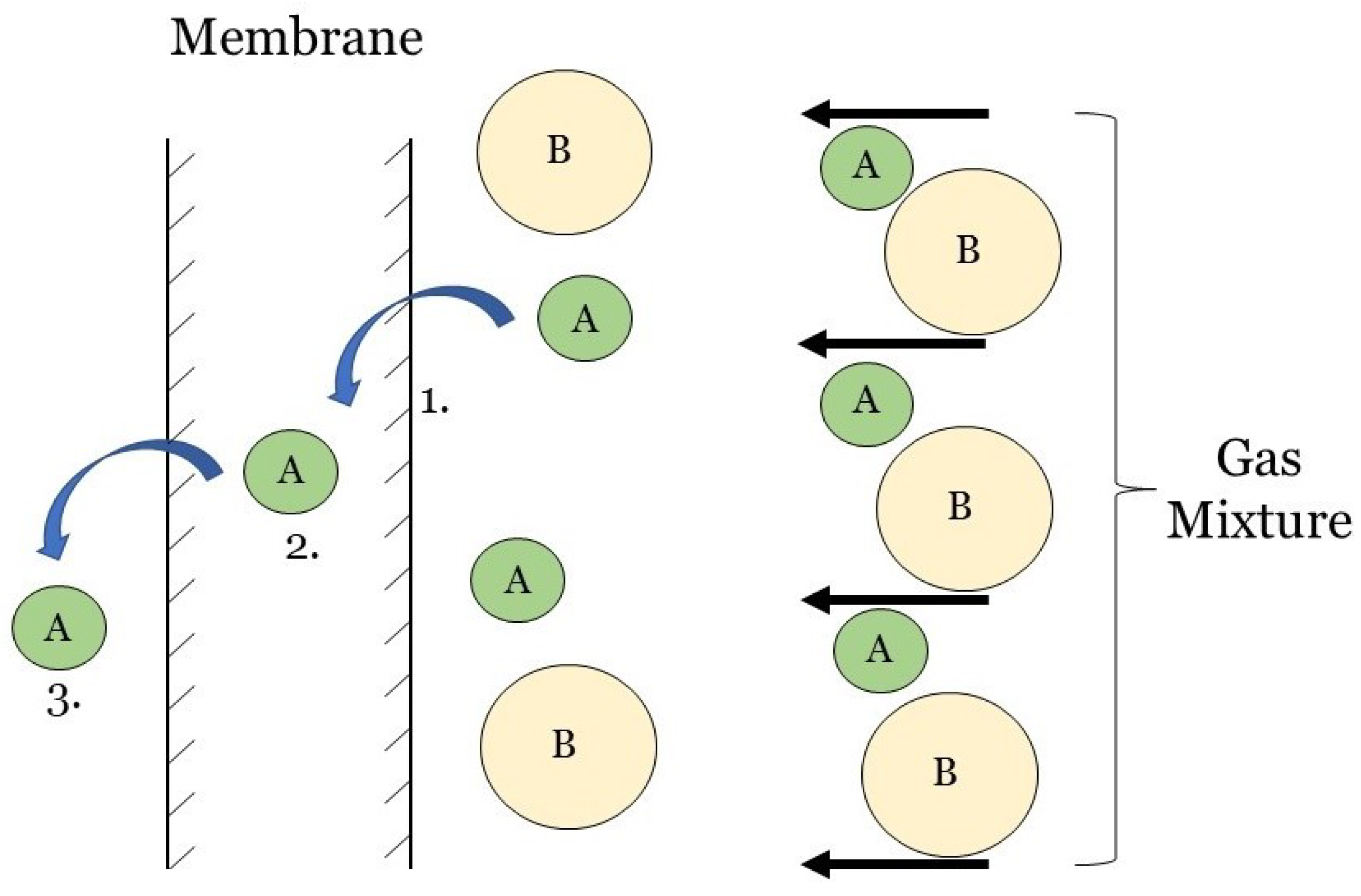
3.2. Solution-Diffusion Model
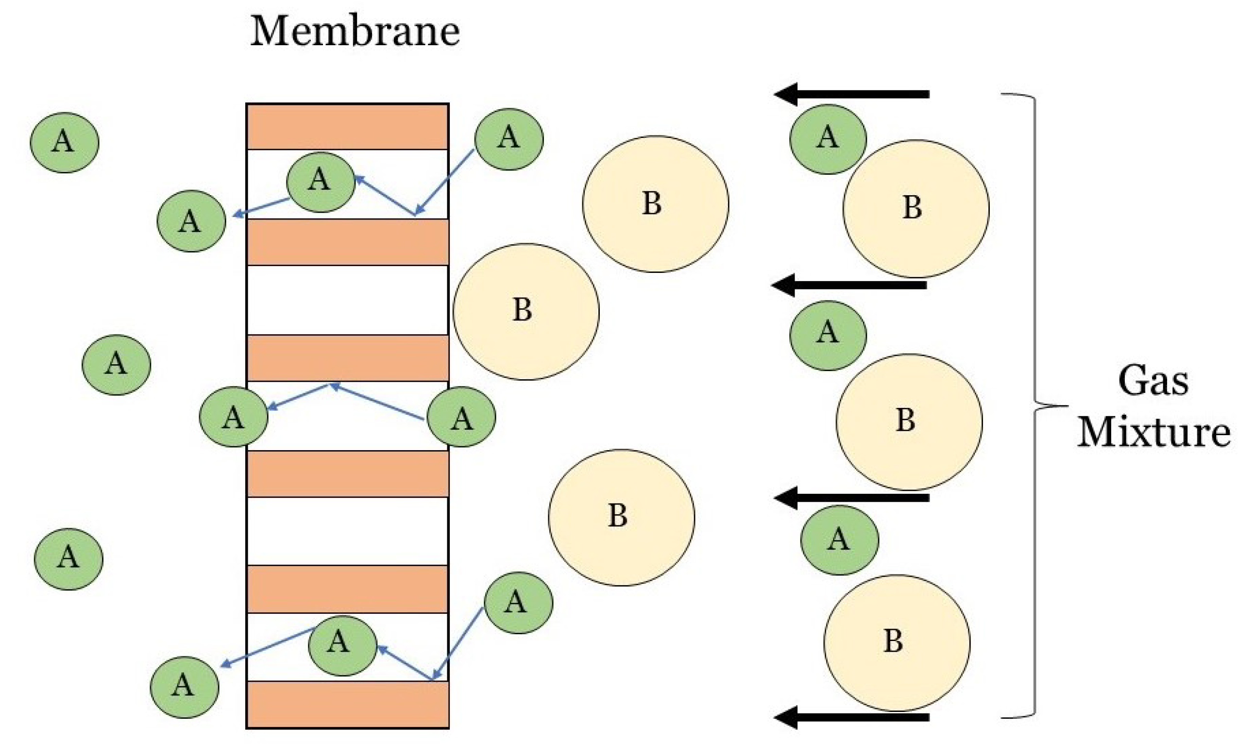
3.3. Pore Flow Model
4. Two-Dimensional Modeling
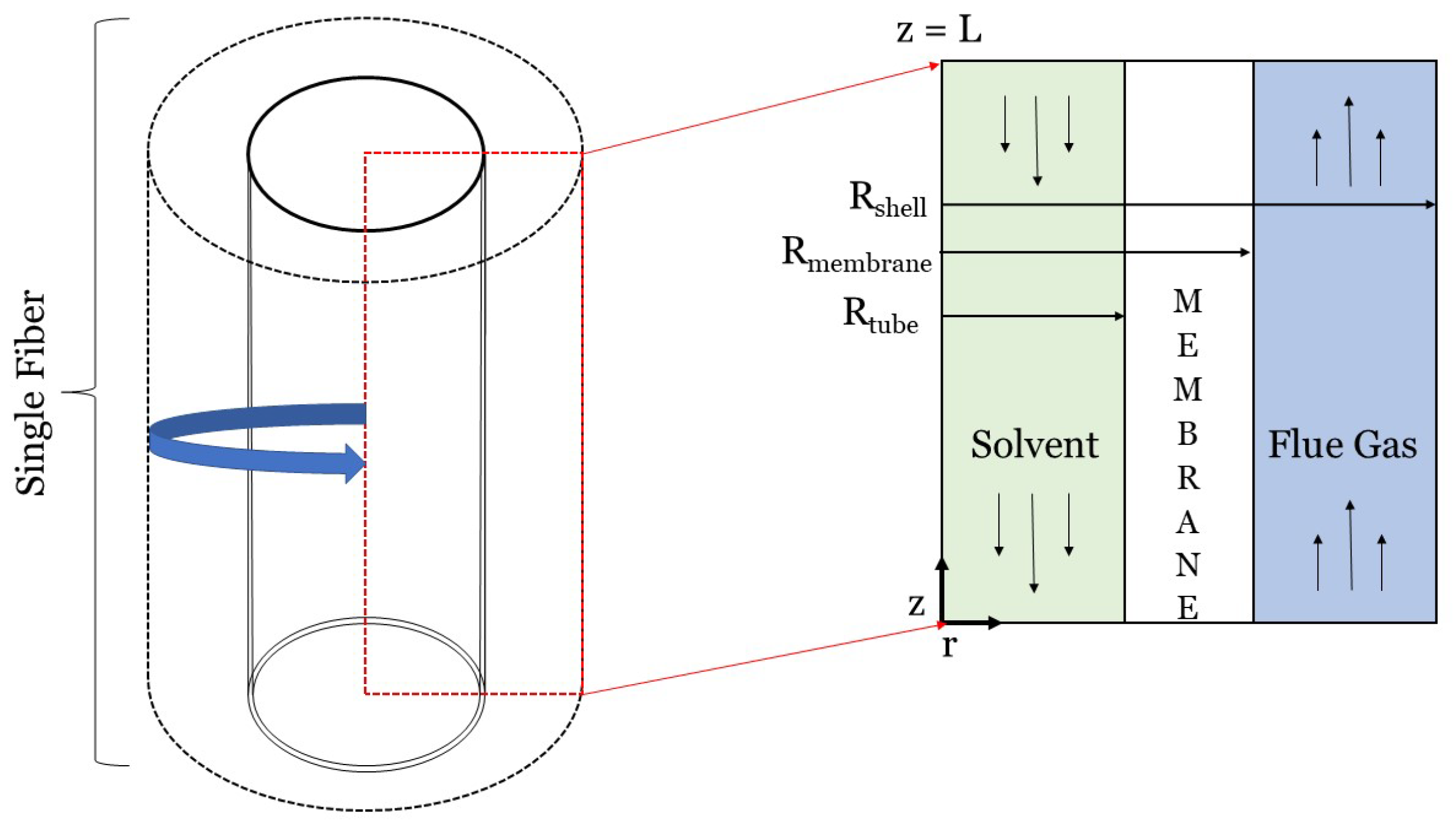
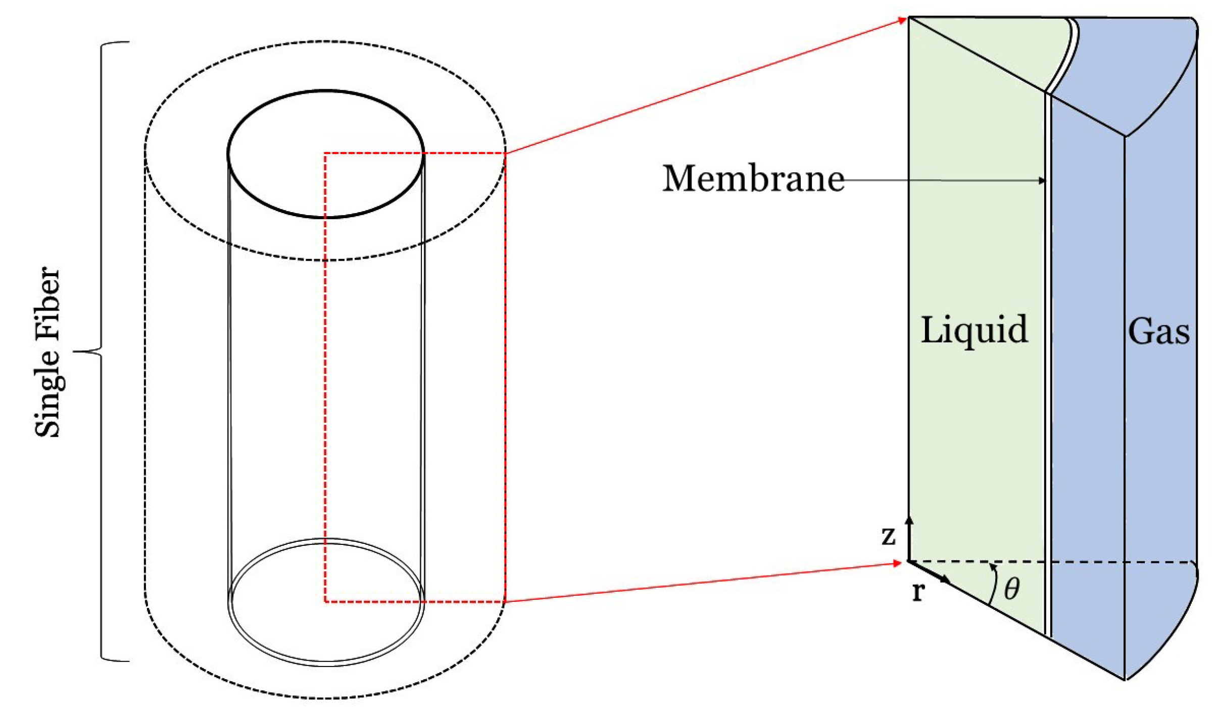
4.1. Governing Equations for a 2D-Axisymmetric HFMC Fiber
4.2. 2D Modeling of Membrane Wetting
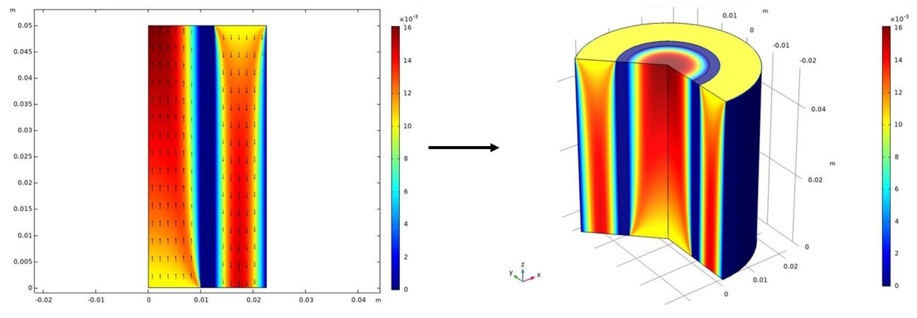
4.3. Benefits of 2D Axisymmetric Modeling
5. Three-Dimensional Modeling
6. Comparison of 1D, 2D, and 3D Modeling Approaches
- Steady-state, laminar, Newtonian, incompressible fluid, and plug flow with fully-developed velocity profiles.
- Ideal gas law (assumes the gas particles are (1) in continuous, rapid motion, (2) are so small that their volume is negligible, (3) do not interact, and (4) temperature is proportional to the average kinetic energy); and Henry’s law (assumes constant temperature and that the vapor phase behaves as an ideal gas).
- Fick’s law of diffusion (assumes constant diffusion coefficient) and thermal conductance through membrane, with adiabatic behavior.
- Rate-controlled reversible reaction.
- Heat and mass transfer are equal at the interface (condensation from the temperature difference occurs at the liquid-membrane interface).
- Uniform membrane properties (constant tortuosity and distribution of membrane pore size, wall thickness, non-wetting).
- Mass transfer between gas-liquid phases is a result of film diffusion.
- Curvature effect of the membrane surface on mass transfer is negligible.
- Happel’s free surface model (assumes the bundle’s porosity is equal to the fluid’s envelope porosity and assumes no friction on the shell-side).
- Initial zero CO concentration on the solvent side.
- Zero mass transfer at the two fiber ends.
- Constant volumetric flow rate.
- Large mass transfer rate between gas and liquid.
- Non-wetted operation in which the gas mixture fills the membrane pores.
- Ideal feed gas (fouling/pollution not accounted for).
- Fibers are rigid walls (no degradation study is needed).
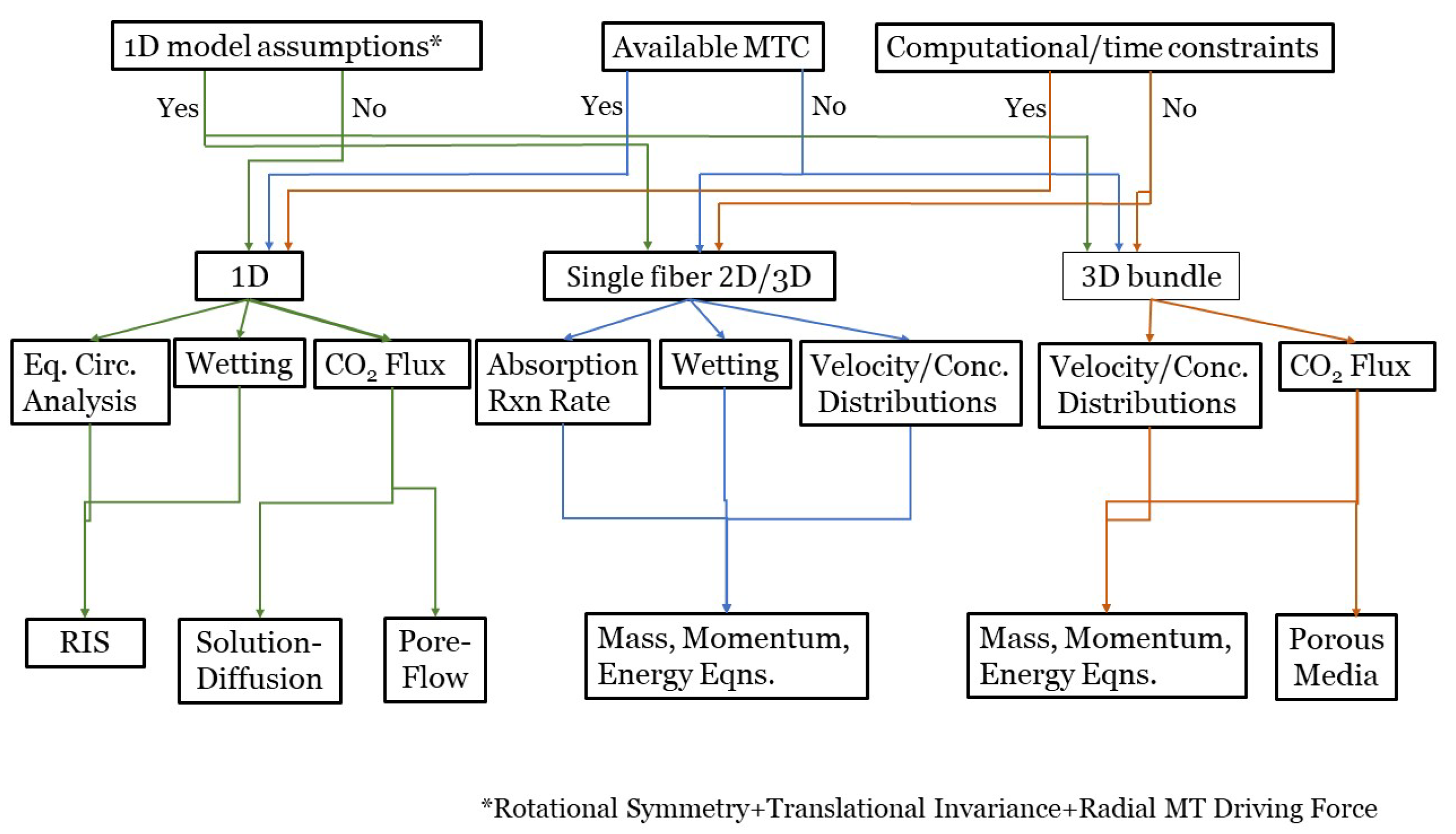
7. HFMC Modeling Road Map
8. Applications and Challenges
8.1. Applications of 1D Models
8.2. Applications of 2D Models
8.3. Applications of 3D Models
8.4. Software Implementations
8.5. Modeling Challenges
9. Scale-Up Modeling from Lab Scale to Commercial Scale
10. Conclusions and Recommended Future Work
Author Contributions
Funding
Acknowledgments
Conflicts of Interest
Nomenclature
| Subscripts | |
| l | liquid |
| m | membrane |
| g | gas |
| ov | overall |
| eff | effective |
| i | inner |
| o | outer |
| h | hydraulic |
| w | liquid pore |
| f | membrane pore |
| max | maximum |
| r | radial coordinate |
| CO | CO in a domain |
| tangential | |
| z | axial coordinate |
| avg | average |
| A | component |
| rxn | reaction |
| t | time |
| i | domain |
| th | thermal |
| j | species |
| Variables | |
| k | resistance |
| D | diffusion coefficient |
| porosity | |
| tortuosity | |
| thickness | |
| d | diameter |
| E | enhancement factor |
| L | length |
| C | concentration |
| R | fixed radius |
| r | reaction rate constant |
| volume fraction | |
| surface tension | |
| m | solubility of CO |
| V | volume |
| surface tension | |
| Darcy permeability | |
| inertial permeability | |
| wetting ratio | |
| velocity vector | |
| volumetric flow rate | |
| effective capture ratio | |
| a | interfacial area |
| H | Henry’s constant |
| P | partial pressure |
| B | pore geometry coefficient |
| T | temperature |
| contact angle | |
| n | number of fibers |
| density | |
| viscosity | |
| gravity | |
| molar flow rate | |
| ∂ | partial differential |
| ▵ | difference |
| body force vector | |
| gradient of velocity | |
| f | constitutive parameter |
| Acronyms | |
| HFM | Hollow fiber membrane |
| HFMC | HFM contactor |
| CC | Carbon capture |
| PCC | Post-combustion carbon capture |
| RIS | Resistance in series |
| MTC | Mass transfer coefficient |
| CFD | Computational Fluid Dynamics |
References
- Allen, M. Chapter 1 Framing and Context; Intergovernmental Panel on Climate Change: Geneva, Switzerland, 2018. [Google Scholar]
- Le Quéré, C.; Andrew, R.M.; Friedlingstein, P.; Sitch, S.; Hauck, J.; Pongratz, J.; Pickers, P.A.; Korsbakken, J.I.; Peters, G.P.; Canadell, J.G.; et al. Global carbon budget 2018. Earth Syst. Sci. Data 2018, 10, 2141–2194. [Google Scholar]
- Energy Information Administration. Monthly Energy Review Energy Information Administration. Total Energy 2020. Available online: https://www.eia.gov/totalenergy/data/monthly/ (accessed on 30 November 2020).
- Echevarria Huaman, R.N. A Review on: CO2 Capture Technology on Fossil Fuel Power Plant. J. Fundam. Renew. Energy Appl. 2015, 5, 3. [Google Scholar] [CrossRef]
- Zhang, Y.; Sunarso, J.; Liu, S.; Wang, R. Current status and development of membranes for CO2/CH4 separation: A review. Int. J. Greenh. Gas Control. 2013, 12, 84–107. [Google Scholar] [CrossRef]
- Drioli, E.; Criscuoli, A.; Curcio, E. Membrane Contactors: Fundamentals, Applications and Potentialities; Elsevier: Amsterdam, The Netherlands, 2011. [Google Scholar]
- Luis, P. Fundamental Modeling of Membrane Systems: Membrane and Process Performance; Elsevier: Amsterdam, The Netherlands, 2018. [Google Scholar]
- Bazhenov, S.; Bildyukevich, A.; Volkov, A. Gas-liquid hollow fiber membrane contactors for different applications. Fibers 2018, 6, 76. [Google Scholar] [CrossRef]
- He, X. A review of material development in the field of carbon capture and the application of membrane-based processes in power plants and energy-intensive industries. Energy Sustain. Soc. 2018, 8, 34. [Google Scholar] [CrossRef]
- Ze, Z.; Sx, J. Hollow fiber membrane contactor absorption of CO2 from the flue gas: review and perspective. Glob. Nest J. 2014, 16, 355–374. [Google Scholar]
- Ismail, A.F.; David, L. A review on the latest development of carbon membranes for gas separation. J. Membr. Sci. 2001, 193, 1–18. [Google Scholar] [CrossRef]
- He, X. The latest development on membrane materials and processes for post-combustion CO2 capture: A review. SF J. Material Chem. Eng. 2018, 1, 1009. [Google Scholar]
- Brunetti, A.; Scura, F.; Barbieri, G.; Drioli, E. Membrane technologies for CO2 separation. J. Membr. Sci. 2010, 359, 115–125. [Google Scholar] [CrossRef]
- Al-Marzouqi, M.H.; El-Naas, M.H.; Marzouk, S.A.; Al-Zarooni, M.A.; Abdullatif, N.; Faiz, R. Modeling of CO2 absorption in membrane contactors. Sep. Purif. Technol. 2008, 59, 286–293. [Google Scholar] [CrossRef]
- Faiz, R.; Al-Marzouqi, M. CO2 removal from natural gas at high pressure using membrane contactors: model validation and membrane parametric studies. J. Membr. Sci. 2010, 365, 232–241. [Google Scholar] [CrossRef]
- Boributh, S.; Assabumrungrat, S.; Laosiripojana, N.; Jiraratananon, R. A modeling study on the effects of membrane characteristics and operating parameters on physical absorption of CO2 by hollow fiber membrane contactor. J. Membr. Sci. 2011, 380, 21–33. [Google Scholar] [CrossRef]
- Boributh, S.; Jiraratananon, R.; Li, K. Analytical solutions for membrane wetting calculations based on log-normal and normal distribution functions for CO2 absorption by a hollow fiber membrane contactor. J. Membr. Sci. 2013, 429, 459–472. [Google Scholar] [CrossRef]
- Boributh, S.; Rongwong, W.; Assabumrungrat, S.; Laosiripojana, N.; Jiraratananon, R. Mathematical modeling and cascade design of hollow fiber membrane contactor for CO2 absorption by monoethanolamine. J. Membr. Sci. 2012, 401, 175–189. [Google Scholar] [CrossRef]
- Chabanon, E.; Roizard, D.; Favre, E. Modeling strategies of membrane contactors for post-combustion carbon capture: a critical comparative study. Chem. Eng. Sci. 2013, 87, 393–407. [Google Scholar] [CrossRef]
- Faiz, R.; El-Naas, M.H.; Al-Marzouqi, M. Significance of gas velocity change during the transport of CO2 through hollow fiber membrane contactors. Chem. Eng. J. 2011, 168, 593–603. [Google Scholar] [CrossRef]
- Khaisri, S.; de Montigny, D.; Tontiwachwuthikul, P.; Jiraratananon, R. A mathematical model for gas absorption membrane contactors that studies the effect of partially wetted membranes. J. Membr. Sci. 2010, 347, 228–239. [Google Scholar] [CrossRef]
- Faiz, R.; Al-Marzouqi, M. Mathematical modeling for the simultaneous absorption of CO2 and H2S using MEA in hollow fiber membrane contactors. J. Membr. Sci. 2009, 342, 269–278. [Google Scholar] [CrossRef]
- Sohrabi, M.R.; Marjani, A.; Moradi, S.; Davallo, M.; Shirazian, S. Mathematical modeling and numerical simulation of CO2 transport through hollow-fiber membranes. Appl. Math. Model. 2011, 35, 174–188. [Google Scholar] [CrossRef]
- Paul, S.; Ghoshal, A.K.; Mandal, B. Removal of CO2 by single and blended aqueous alkanolamine solvents in hollow-fiber membrane contactor: Modeling and simulation. Ind. Eng. Chem. Res. 2007, 46, 2576–2588. [Google Scholar] [CrossRef]
- Zhang, H.Y.; Wang, R.; Liang, D.T.; Tay, J.H. Theoretical and experimental studies of membrane wetting in the membrane gas–liquid contacting process for CO2 absorption. J. Membr. Sci. 2008, 308, 162–170. [Google Scholar] [CrossRef]
- Goyal, N.; Suman, S.; Gupta, S. Mathematical modeling of CO2 separation from gaseous-mixture using a Hollow-Fiber Membrane Module: Physical mechanism and influence of partial-wetting. J. Membr. Sci. 2015, 474, 64–82. [Google Scholar] [CrossRef]
- Wang, R.; Li, D.; Liang, D. Modeling of CO2 capture by three typical amine solutions in hollow fiber membrane contactors. Chem. Eng. Process. Process. Intensif. 2004, 43, 849–856. [Google Scholar] [CrossRef]
- Dindore, V.; Brilman, D.W.F.; Versteeg, G. Hollow fiber membrane contactor as a gas–liquid model contactor. Chem. Eng. Sci. 2005, 60, 467–479. [Google Scholar] [CrossRef]
- Mansourizadeh, A.; Ismail, A.; Matsuura, T. Effect of operating conditions on the physical and chemical CO2 absorption through the PVDF hollow fiber membrane contactor. J. Membr. Sci. 2010, 353, 192–200. [Google Scholar] [CrossRef]
- Rezakazemi, M.; Niazi, Z.; Mirfendereski, M.; Shirazian, S.; Mohammadi, T.; Pak, A. CFD simulation of natural gas sweetening in a gas–liquid hollow-fiber membrane contactor. Chem. Eng. J. 2011, 168, 1217–1226. [Google Scholar] [CrossRef]
- Shirazian, S.; Pishnamazi, M.; Rezakazemi, M.; Nouri, A.; Jafari, M.; Noroozi, S.; Marjani, A. Implementation of the finite element method for simulation of mass transfer in membrane contactors. Chem. Eng. Technol. 2012, 35, 1077–1084. [Google Scholar] [CrossRef]
- Hoff, K.A.; Juliussen, O.; Falk-Pedersen, O.; Svendsen, H.F. Modeling and experimental study of carbon dioxide absorption in aqueous alkanolamine solutions using a membrane contactor. Ind. Eng. Chem. Res. 2004, 43, 4908–4921. [Google Scholar] [CrossRef]
- Dindore, V.; Brilman, D.W.F.; Versteeg, G. Modelling of cross-flow membrane contactors: Mass transfer with chemical reactions. J. Membr. Sci. 2005, 255, 275–289. [Google Scholar] [CrossRef]
- Marzouk, S.A.; Al-Marzouqi, M.H.; El-Naas, M.H.; Abdullatif, N.; Ismail, Z.M. Removal of carbon dioxide from pressurized CO2–CH4 gas mixture using hollow fiber membrane contactors. J. Membr. Sci. 2010, 351, 21–27. [Google Scholar] [CrossRef]
- Farjami, M.; Moghadassi, A.; Vatanpour, V. Modeling and simulation of CO2 removal in a polyvinylidene fluoride hollow fiber membrane contactor with computational fluid dynamics. Chem. Eng. Process. Process. Intensif. 2015, 98, 41–51. [Google Scholar] [CrossRef]
- Mehdipourghazi, M.; Barati, S.; Varaminian, F. Mathematical modeling and simulation of carbon dioxide stripping from water using hollow fiber membrane contactors. Chem. Eng. Process. Process. Intensif. 2015, 95, 159–164. [Google Scholar] [CrossRef]
- DashtArzhandi, M.R.; Ismail, A.; Matsuura, T. Carbon dioxide stripping through water by porous PVDF/montmorillonite hollow fiber mixed matrix membranes in a membrane contactor. RSC Adv. 2015, 5, 21916–21924. [Google Scholar] [CrossRef]
- Dong, X.; Wu, H.C.; Lin, Y. CO2 permeation through asymmetric thin tubular ceramic-carbonate dual-phase membranes. J. Membr. Sci. 2018, 564, 73–81. [Google Scholar] [CrossRef]
- Han, Y.; Salim, W.; Chen, K.K.; Wu, D.; Ho, W.W. Field trial of spiral-wound facilitated transport membrane module for CO2 capture from flue gas. J. Membr. Sci. 2019, 575, 242–251. [Google Scholar] [CrossRef]
- Brinkmann, T.; Notzke, H.; Wolff, T.; Zhao, L.; Luhr, S.; Stolten, D. Characterization of a New Flat Sheet Membrane Module Type for Gas Permeation. Chem. Ing. Tech. 2019, 91, 30–37. [Google Scholar] [CrossRef]
- Mat, N.C.; Lou, Y.; Lipscomb, G.G. Hollow fiber membrane modules. Curr. Opin. Chem. Eng. 2014, 4, 18–24. [Google Scholar] [CrossRef]
- Wan, C.F.; Yang, T.; Lipscomb, G.G.; Stookey, D.J.; Chung, T.S. Design and fabrication of hollow fiber membrane modules. J. Membr. Sci. 2017, 538, 96–107. [Google Scholar] [CrossRef]
- Shirazian, S.; Moghadassi, A.; Moradi, S. Numerical simulation of mass transfer in gas–liquid hollow fiber membrane contactors for laminar flow conditions. Simul. Model. Pract. Theory 2009, 17, 708–718. [Google Scholar] [CrossRef]
- Zhao, S.; Feron, P.H.; Deng, L.; Favre, E.; Chabanon, E.; Yan, S.; Hou, J.; Chen, V.; Qi, H. Status and progress of membrane contactors in post-combustion carbon capture: A state-of-the-art review of new developments. J. Membr. Sci. 2016, 511, 180–206. [Google Scholar] [CrossRef]
- Gabelman, A.; Hwang, S.T. Hollow fiber membrane contactors. J. Membr. Sci. 1999, 159, 61–106. [Google Scholar] [CrossRef]
- Ji, G.; Zhao, M. Membrane separation technology in carbon capture. In Recent Advances in Carbon Capture and Storage; Yun, Y., Ed.; IntechOpen: London, UK, 2017; pp. 59–90. [Google Scholar]
- Wang, Y.; Zhao, L.; Otto, A.; Robinius, M.; Stolten, D. A Review of Post-combustion CO2 Capture Technologies from Coal-fired Power Plants. Energy Procedia 2017, 114, 650–665. [Google Scholar] [CrossRef]
- Pabby, A.K.; Sastre, A.M. State-of-the-art review on hollow fibre contactor technology and membrane-based extraction processes. J. Membr. Sci. 2013, 430, 263–303. [Google Scholar] [CrossRef]
- Mondal, M.K.; Balsora, H.K.; Varshney, P. Progress and trends in CO2 capture/separation technologies: A review. Energy 2012, 46, 431–441. [Google Scholar] [CrossRef]
- Li, B.; Duan, Y.; Luebke, D.; Morreale, B. Advances in CO2 capture technology: A patent review. Appl. Energy 2013, 102, 1439–1447. [Google Scholar] [CrossRef]
- Cui, Z.; de Montigny, D. Part 7: A review of CO2 capture using hollow fiber membrane contactors. Carbon Manag. 2013, 4, 69–89. [Google Scholar] [CrossRef]
- Khalilpour, R.; Mumford, K.; Zhai, H.; Abbas, A.; Stevens, G.; Rubin, E.S. Membrane-based carbon capture from flue gas: A review. J. Clean. Prod. 2015, 103, 286–300. [Google Scholar] [CrossRef]
- None, N. The National Carbon Capture Center at the Power Systems Development Facility; Technical Report; Southern Company Services Incorporated: Wilsonville, AL, USA, 2014. [Google Scholar]
- He, X.; Hägg, M.B. Hollow fiber carbon membranes: Investigations for CO2 capture. J. Membr. Sci. 2011, 378, 1–9. [Google Scholar] [CrossRef]
- Bird, R.B.; Stewart, W.E.; Lightfoot, E.N. Transport Phenomena, rev. 2nd ed.; J. Wiley: New York, NY, USA, 2007. [Google Scholar]
- Slattery, J.C. Advanced Transport Phenomena; Cambridge University Press: Cambridge, UK, 1999. [Google Scholar]
- Uguz, A.K.; Massoudi, M. Heat transfer and Couette flow of a chemically reacting non-linear fluid. Math. Methods Appl. Sci. 2010, 33, 1331–1341. [Google Scholar] [CrossRef]
- Massoudi, M.; Uguz, A. Chemically-reacting fluids with variable transport properties. Appl. Math. Comput. 2012, 219, 1761–1775. [Google Scholar] [CrossRef]
- Coker, D.; Allen, T.; Freeman, B.D.; Fleming, G. Nonisothermal model for gas separation hollow-fiber membranes. AIChE J. 1999, 45, 1451–1468. [Google Scholar] [CrossRef]
- Shirazian, S.; Ashrafizadeh, S. Mass transfer simulation of carbon dioxide absorption in a hollow-fiber membrane contactor. Sep. Sci. Technol. 2010, 45, 515–524. [Google Scholar] [CrossRef]
- Razavi, S.M.R.; Shirazian, S.; Nazemian, M. Numerical simulation of CO2 separation from gas mixtures in membrane modules: Effect of chemical absorbent. Arab. J. Chem. 2016, 9, 62–71. [Google Scholar] [CrossRef]
- Pahlavanzadeh, H.; Darabi, M.; Ghaleh, V.R.; Bakhtiari, O. CFD Modeling of CO2 Absorption in Membrane Contactors Using Aqueous Solutions of Monoethanolamine–Ionic Liquids. Ind. Eng. Chem. Res. 2020, 59, 18629–18639. [Google Scholar] [CrossRef]
- Qazi, S.; Gómez-Coma, L.; Albo, J.; Druon-Bocquet, S.; Irabien, A.; Sanchez-Marcano, J. CO2 capture in a hollow fiber membrane contactor coupled with ionic liquid: Influence of membrane wetting and process parameters. Sep. Purif. Technol. 2020, 233, 115986. [Google Scholar] [CrossRef]
- Abdolahi-Mansoorkhani, H.; Seddighi, S. CO2 capture by modified hollow fiber membrane contactor: Numerical study on membrane structure and membrane wettability. Fuel Process. Technol. 2020, 209, 106530. [Google Scholar] [CrossRef]
- Ghasem, N. Modeling and Simulation of the Simultaneous Absorption/Stripping of CO2 with Potassium Glycinate Solution in Membrane Contactor. Membranes 2020, 10, 72. [Google Scholar] [CrossRef]
- Bruus, H. Theoretical Microfluidics, rev. 2nd ed.; Oxford University Press Inc.: New York, NY, USA, 2009. [Google Scholar]
- Wickramasinghe, S.; Semmens, M.J.; Cussler, E. Mass-Transfer in Various Hollow Fiber Geometries. J. Membr. Sci. 1992, 69, 235–250. [Google Scholar] [CrossRef]
- Boributh, S.; Assabumrungrat, S.; Laosiripojana, N.; Jiraratananon, R. Effect of membrane module arrangement of gas–liquid membrane contacting process on CO2 absorption performance: A modeling study. J. Membr. Sci. 2011, 372, 75–86. [Google Scholar] [CrossRef]
- Henis, J.M.; Tripodi, M.K. Composite hollow fiber membranes for gas separation: The resistance model approach. J. Membr. Sci. 1981, 8, 233–246. [Google Scholar] [CrossRef]
- Baker, R.W. Membrane Technology and Applications; John Wiley & Sons: Hoboken, NJ, USA, 2012. [Google Scholar]
- Mavroudi, M.; Kaldis, S.; Sakellaropoulos, G. A study of mass transfer resistance in membrane gas–liquid contacting processes. J. Membr. Sci. 2006, 272, 103–115. [Google Scholar] [CrossRef]
- Saeed, M.; Deng, L. Post-combustion CO2 membrane absorption promoted by mimic enzyme. J. Membr. Sci. 2016, 499, 36–46. [Google Scholar] [CrossRef]
- Rode, S.; Nguyen, P.T.; Roizard, D.; Bounaceur, R.; Castel, C.; Favre, E. Evaluating the intensification potential of membrane contactors for gas absorption in a chemical solvent: A generic one-dimensional methodology and its application to CO2 absorption in monoethanolamine. J. Membr. Sci. 2012, 389, 1–16. [Google Scholar] [CrossRef]
- Mulder, M. Basic Principles of Membrane Technology; Springer Science & Business Media: Berlin/Heidelberg, Germany, 2012. [Google Scholar]
- Kreulen, H.; Smolders, C.; Versteeg, G.; Van Swaaij, W.P.M. Determination of mass transfer rates in wetted and non-wetted microporous membranes. Chem. Eng. Sci. 1993, 48, 2093–2102. [Google Scholar] [CrossRef]
- Yang, M.C.; Cussler, E. Designing hollow-fiber contactors. AIChE J. 1986, 32, 1910–1916. [Google Scholar] [CrossRef]
- Qi, Z.; Cussler, E. Microporous hollow fibers for gas absorption: I. Mass transfer in the liquid. J. Membr. Sci. 1985, 23, 321–332. [Google Scholar] [CrossRef]
- DeCoursey, W. Enhancement factors for gas absorption with reversible reaction. Chem. Eng. Sci. 1982, 37, 1483–1489. [Google Scholar] [CrossRef]
- Kumar, P.; Hogendoorn, J.; Feron, P.; Versteeg, G. Approximate solution to predict the enhancement factor for the reactive absorption of a gas in a liquid flowing through a microporous membrane hollow fiber. J. Membr. Sci. 2003, 213, 231–245. [Google Scholar] [CrossRef]
- Cussler, E.L.; Cussler, E.L. Diffusion: Mass Transfer in Fluid Systems; Cambridge University Press: Cambridge, UK, 2009. [Google Scholar]
- Gaspar, J.; Fosbøl, P.L. Practical enhancement factor model based on GM for multiple parallel reactions: Piperazine (PZ) CO2 capture. Chem. Eng. Sci. 2017, 158, 257–266. [Google Scholar] [CrossRef]
- Li, J.L.; Chen, B.H. Review of CO2 absorption using chemical solvents in hollow fiber membrane contactors. Sep. Purif. Technol. 2005, 41, 109–122. [Google Scholar] [CrossRef]
- Rongwong, W.; Jiraratananon, R.; Atchariyawut, S. Experimental study on membrane wetting in gas–liquid membrane contacting process for CO2 absorption by single and mixed absorbents. Sep. Purif. Technol. 2009, 69, 118–125. [Google Scholar] [CrossRef]
- Atchariyawut, S.; Feng, C.; Wang, R.; Jiraratananon, R.; Liang, D. Effect of membrane structure on mass-transfer in the membrane gas–liquid contacting process using microporous PVDF hollow fibers. J. Membr. Sci. 2006, 285, 272–281. [Google Scholar] [CrossRef]
- Li, Y.; Jin, P.; Song, X.; Zhan, X. Removal of carbon dioxide from pressurized landfill gas by physical absorbents using a hollow fiber membrane contactor. Chem. Eng. Process. Process. Intensif. 2017, 121, 149–161. [Google Scholar] [CrossRef]
- Mosadegh-Sedghi, S.; Rodrigue, D.; Brisson, J.; Iliuta, M.C. Wetting phenomenon in membrane contactors–causes and prevention. J. Membr. Sci. 2014, 452, 332–353. [Google Scholar] [CrossRef]
- Kreulen, H.; Smolders, C.; Versteeg, G.; van Swaaij, W.P.M. Microporous hollow fibre membrane modules as gas-liquid contactors Part 2. Mass transfer with chemical reaction. J. Membr. Sci. 1993, 78, 217–238. [Google Scholar] [CrossRef]
- Scholes, C.A.; Qader, A.; Stevens, G.W.; Kentish, S.E. Membrane gas-solvent contactor pilot plant trials of CO2 absorption from flue gas. Sep. Sci. Technol. 2014, 49, 2449–2458. [Google Scholar] [CrossRef]
- Rezaei, M.; Warsinger, D.M.; Duke, M.C.; Matsuura, T.; Samhaber, W.M. Wetting phenomena in membrane distillation: Mechanisms, reversal, and prevention. Water Res. 2018, 139, 329–352. [Google Scholar] [CrossRef]
- Franken, A.; Nolten, J.; Mulder, M.; Bargeman, D.; Smolders, C. Wetting criteria for the applicability of membrane distillation. J. Membr. Sci. 1987, 33, 315–328. [Google Scholar] [CrossRef]
- Khalilpour, R.; Abbas, A.; Lai, Z.; Pinnau, I. Modeling and parametric analysis of hollow fiber membrane system for carbon capture from multicomponent flue gas. AIChE J. 2012, 58, 1550–1561. [Google Scholar] [CrossRef]
- Ismail, A.F.; Kusworo, T.; Mustafa, A.; Hasbulla, H. Understanding the solution-diffusion mechanism in gas separation membrane for engineering students. In Proceedings of the Regional Conference on Engineering Education RCEE, Johor, Malaysia, 2005; Volume 20052005. [Google Scholar]
- Alkhouzaam, A.; Khraisheh, M.; Atilhan, M.; Al-Muhtaseb, S.A.; Qi, L.; Rooney, D. High-pressure CO2/N2 and CO2/CH4 separation using dense polysulfone-supported ionic liquid membranes. J. Nat. Gas Sci. Eng. 2016, 36, 472–485. [Google Scholar] [CrossRef]
- Wijmans, J.G.; Baker, R.W. The Solution-Diffusion Model: A Review. J. Memb. Sci. 1995, 107, 1–21. [Google Scholar] [CrossRef]
- Mauviel, G.; Berthiaud, J.; Vallieres, C.; Roizard, D.; Favre, E. Dense membrane permeation: From the limitations of the permeability concept back to the solution-diffusion model. J. Membr. Sci. 2005, 266, 62–67. [Google Scholar] [CrossRef]
- Chu, Y.; Lindbråthen, A.; Lei, L.; He, X.; Hillestad, M. Mathematical modeling and process parametric study of CO2 removal from natural gas by hollow fiber membranes. Chem. Eng. Res. Des. 2019, 148, 45–55. [Google Scholar] [CrossRef]
- Zaidiza, D.A.; Belaissaoui, B.; Rode, S.; Neveux, T.; Makhloufi, C.; Castel, C.; Roizard, D.; Favre, E. Adiabatic modelling of CO2 capture by amine solvents using membrane contactors. J. Membr. Sci. 2015, 493, 106–119. [Google Scholar] [CrossRef]
- Bottino, A.; Capannelli, G.; Comite, A.; Di Felice, R.; Firpo, R. CO2 removal from a gas stream by membrane contactor. Sep. Purif. Technol. 2008, 59, 85–90. [Google Scholar] [CrossRef]
- Villeneuve, K.; Zaidiza, D.A.; Roizard, D.; Rode, S. Modeling and simulation of CO2 capture in aqueous ammonia with hollow fiber composite membrane contactors using a selective dense layer. Chem. Eng. Sci. 2018, 190, 345–360. [Google Scholar] [CrossRef]
- Leiknes, T. Theory of Transport in Membrane. Ph.D. Thesis, King Abdullah University of Science and Technology, Thuwal, Saudi Arabia; pp. 1–17.
- Zaidiza, D.A.; Billaud, J.; Belaissaoui, B.; Rode, S.; Roizard, D.; Favre, E. Modeling of CO2 post-combustion capture using membrane contactors, comparison between one-and two-dimensional approaches. J. Membr. Sci. 2014, 455, 64–74. [Google Scholar] [CrossRef]
- Haddadi, B.; Jordan, C.; Miltner, M.; Harasek, M. Membrane modeling using CFD: Combined evaluation of mass transfer and geometrical influences in 1D and 3D. J. Membr. Sci. 2018, 563, 199–209. [Google Scholar] [CrossRef]
- Zhang, H.Y.; Wang, R.; Liang, D.T.; Tay, J.H. Modeling and experimental study of CO2 absorption in a hollow fiber membrane contactor. J. Membr. Sci. 2006, 279, 301–310. [Google Scholar] [CrossRef]
- Nakhjiri, A.T.; Heydarinasab, A.; Bakhtiari, O.; Mohammadi, T. Numerical simulation of CO2/H2S simultaneous removal from natural gas using potassium carbonate aqueous solution in hollow fiber membrane contactor. J. Environ. Chem. Eng. 2020, 8, 104130. [Google Scholar] [CrossRef]
- Marjani, A.; Nakhjiri, A.T.; Taleghani, A.S.; Shirazian, S. Mass transfer modeling absorption using nanofluids in porous polymeric membranes. J. Mol. Liq. 2020, 318, 114115. [Google Scholar] [CrossRef]
- Hoff, K.A. Modeling and Experimental Study of Carbon Dioxide Absorption in a Membrane Contactor. Available online: https://www.semanticscholar.org/paper/Modeling-and-Experimental-Study-of-Carbon-Dioxide-a-Hoff/c1bddaf9d881b7550a13843db8e321f1710c7172 (accessed on 30 November 2020).
- Fox, R.W.; McDonald, A.T.; Mitchell, J.W. Fox and McDonald’s Introduction to Fluid Mechanics; John Wiley & Sons: Hoboken, NJ, USA, 2020. [Google Scholar]
- Happel, J. Viscous flow relative to arrays of cylinders. AIChE J. 1959, 5, 174–177. [Google Scholar] [CrossRef]
- Cao, F.; Gao, H.; Ling, H.; Huang, Y.; Liang, Z. Theoretical modeling of the mass transfer performance of CO2 absorption into DEAB solution in hollow fiber membrane contactor. J. Membr. Sci. 2020, 593, 117439. [Google Scholar] [CrossRef]
- Shirazian, S.; Taghvaie Nakhjiri, A.; Heydarinasab, A.; Ghadiri, M. Theoretical investigations on the effect of absorbent type on carbon dioxide capture in hollow-fiber membrane contactors. PLoS ONE 2020, 15, e0236367. [Google Scholar] [CrossRef]
- Ghasem, N.; Al-Marsouqi, M.; Rahim, N.A. Simulation of Gas/Liquid Membrane Contactor via COMSOL Multiphysics®. Available online: https://cn.comsol.com/paper/download/181505/ghasem_paper.pdf (accessed on 30 November 2020).
- Nakhjiri, A.T.; Heydarinasab, A. CFD Analysis of CO2 Sequestration Applying Different Absorbents Inside the Microporous PVDF Hollow Fiber Membrane Contactor. Period. Polytech. Chem. Eng. 2020, 64, 135–145. [Google Scholar] [CrossRef]
- Qazi, S.; Gómez-Coma, L.; Albo, J.; Druon-Bocquet, S.; Irabien, A.; Younas, M.; Sanchez-Marcano, J. Mathematical modeling of CO2 absorption with ionic liquids in a membrane contactor, study of absorption kinetics and influence of temperature. J. Chem. Technol. Biotechnol. 2020, 95, 1844–1857. [Google Scholar] [CrossRef]
- Hosseinzadeh, A.; Hosseinzadeh, M.; Vatani, A.; Mohammadi, T. Mathematical modeling for the simultaneous absorption of CO2 and SO2 using MEA in hollow fiber membrane contactors. Chem. Eng. Process. Process. Intensif. 2017, 111, 35–45. [Google Scholar] [CrossRef]
- Ibrahim, M.H.; El-Naas, M.H.; Zhang, Z.; Van der Bruggen, B. CO2 capture using hollow fiber membranes: A review of membrane wetting. Energy Fuels 2018, 32, 963–978. [Google Scholar] [CrossRef]
- Malek, A.; Li, K.; Teo, W. Modeling of microporous hollow fiber membrane modules operated under partially wetted conditions. Ind. Eng. Chem. Res. 1997, 36, 784–793. [Google Scholar] [CrossRef]
- Lu, J.G.; Zheng, Y.F.; Cheng, M.D. Wetting mechanism in mass transfer process of hydrophobic membrane gas absorption. J. Membr. Sci. 2008, 308, 180–190. [Google Scholar] [CrossRef]
- Bahlake, A.; Farivar, F.; Dabir, B. New 3-dimensional CFD modeling of CO2 and H2S simultaneous stripping from water within PVDF hollow fiber membrane contactor. Heat Mass Transf. 2016, 52, 1295–1304. [Google Scholar] [CrossRef]
- Boucif, N.; Corriou, J.P.; Roizard, D.; Favre, E. Carbon dioxide absorption by monoethanolamine in hollow fiber membrane contactors: A parametric investigation. AIChE J. 2012, 58, 2843–2855. [Google Scholar] [CrossRef]
- Boucif, N.; Roizard, D.; Corriou, J.P.; Favre, E. To What Extent Does Temperature Affect Absorption in Gas-Liquid Hollow Fiber Membrane Contactors? Sep. Sci. Technol. 2015, 50, 1331–1343. [Google Scholar] [CrossRef]
- Usta, M.; Morabito, M.; Alrehili, M.; Hakim, A.; Oztekin, A. Steady three-dimensional flows past hollow fiber membrane arrays–cross flow arrangement. Can. J. Phys. 2018, 96, 1272–1287. [Google Scholar] [CrossRef]
- Zhang, J.; Nolan, T.D.; Zhang, T.; Griffith, B.P.; Wu, Z.J. Characterization of membrane blood oxygenation devices using computational fluid dynamics. J. Membr. Sci. 2007, 288, 268–279. [Google Scholar] [CrossRef]
- Saidi, M.; Hajaligol, M.; Mhaisekar, A.; Subbiah, M. A 3D modeling of static and forward smoldering combustion in a packed bed of materials. Appl. Math. Model. 2007, 31, 1970–1996. [Google Scholar] [CrossRef]
- Motlagh, A.A.; Hashemabadi, S. 3D CFD simulation and experimental validation of particle-to-fluid heat transfer in a randomly packed bed of cylindrical particles. Int. Commun. Heat Mass Transf. 2008, 35, 1183–1189. [Google Scholar] [CrossRef]
- Yang, W.; Wang, Y.; Chen, J.; Fei, W. Computational fluid dynamic simulation of fluid flow in a rotating packed bed. Chem. Eng. J. 2010, 156, 582–587. [Google Scholar] [CrossRef]
- Ergun, S.; Orning, A.A. Fluid flow through randomly packed columns and fluidized beds. Ind. Eng. Chem. 1949, 41, 1179–1184. [Google Scholar] [CrossRef]
- Lim, S.; Liang, Y.; Weihs, G.F.; Wiley, D.; Fletcher, D. A CFD study on the effect of membrane permeance on permeate flux enhancement generated by unsteady slip velocity. J. Membr. Sci. 2018, 556, 138–145. [Google Scholar] [CrossRef]
- Taherinejad, M.; Gorman, J.; Sparrow, E.; Derakhshan, S. Porous medium model of a hollow-fiber water filtration system. J. Membr. Sci. 2018, 563, 210–220. [Google Scholar] [CrossRef]
- Fill, B.J.; Gartner, M.J.; Johnson, G.; Ma, J.; Horner, M. Porous media technique for computational modeling of a novel pump-oxygenator. Asaio J. 2006, 52, 28A. [Google Scholar] [CrossRef]
- Svitek, R.; Federspiel, W. A mathematical model to predict CO2 removal in hollow fiber membrane oxygenators. Ann. Biomed. Eng. 2008, 36, 992–1003. [Google Scholar] [CrossRef] [PubMed]
- Zaidiza, D.A.; Wilson, S.G.; Belaissaoui, B.; Rode, S.; Castel, C.; Roizard, D.; Favre, E. Rigorous modelling of adiabatic multicomponent CO2 post-combustion capture using hollow fibre membrane contactors. Chem. Eng. Sci. 2016, 145, 45–58. [Google Scholar] [CrossRef]
- Bao, L.; Lipscomb, G. Mass transfer in axial flows through randomly packed fiber bundles. In Membrane Science and Technology; Elsevier: Amsterdam, The Netherlands, 2003; Volume 8, pp. 5–26. [Google Scholar]
- Cai, J.J.; Hawboldt, K.; Abdi, M.A. Analysis of the effect of module design on gas absorption in cross flow hollow membrane contactors via computational fluid dynamics (CFD) analysis. J. Membr. Sci. 2016, 520, 415–424. [Google Scholar] [CrossRef]
- Mazaheri, A.R.; Ahmadi, G. Uniformity of the fluid flow velocities within hollow fiber membranes of blood oxygenation devices. Artif. Organs 2006, 30, 10–15. [Google Scholar] [CrossRef]
- Zaidiza, D.A.; Belaissaoui, B.; Rode, S.; Favre, E. Intensification potential of hollow fiber membrane contactors for CO2 chemical absorption and stripping using monoethanolamine solutions. Sep. Purif. Technol. 2017, 188, 38–51. [Google Scholar] [CrossRef]
- Pozzobon, V.; Perré, P. Mass transfer in hollow fiber membrane contactor: Computational fluid dynamics determination of the shell side resistance. Sep. Purif. Technol. 2020, 241, 116674. [Google Scholar] [CrossRef]
- Villeneuve, K.; Roizard, D.; Remigy, J.C.; Iacono, M.; Rode, S. CO2 capture by aqueous ammonia with hollow fiber membrane contactors: Gas phase reactions and performance stability. Sep. Purif. Technol. 2018, 199, 189–197. [Google Scholar] [CrossRef]
- Whitaker, S. Forced convection heat transfer correlations for flow in pipes, past flat plates, single cylinders, single spheres, and for flow in packed beds and tube bundles. AIChE J. 1972, 18, 361–371. [Google Scholar] [CrossRef]
- Fougerit, V.; Pozzobon, V.; Pareau, D.; Théoleyre, M.A.; Stambouli, M. Gas-liquid absorption in industrial cross-flow membrane contactors: Experimental and numerical investigation of the influence of transmembrane pressure on partial wetting. Chem. Eng. Sci. 2017, 170, 561–573. [Google Scholar] [CrossRef]
- Fougerit, V.; Pozzobon, V.; Pareau, D.; Théoleyre, M.A.; Stambouli, M. Experimental and numerical investigation binary mixture mass transfer in a gas–Liquid membrane contactor. J. Membr. Sci. 2019, 572, 1–11. [Google Scholar] [CrossRef]
- Belaissaoui, B.; Favre, E. Novel dense skin hollow fiber membrane contactor based process for CO2 removal from raw biogas using water as absorbent. Sep. Purif. Technol. 2018, 193, 112–126. [Google Scholar] [CrossRef]
- Ahmad, F.; Lau, K.K.; Lock, S.S.M.; Rafiq, S.; Khan, A.U.; Lee, M. Hollow fiber membrane model for gas separation: Process simulation, experimental validation and module characteristics study. J. Ind. Eng. Chem. 2015, 21, 1246–1257. [Google Scholar] [CrossRef]
- Vogt, M.; Goldschmidt, R.; Bathen, D.; Epp, B.; Fahlenkamp, H. Comparison of membrane contactor and structured packings for CO2 absorption. Energy Procedia 2011, 4, 1471–1477. [Google Scholar] [CrossRef]
- Scholes, C.A.; Simioni, M.; Qader, A.; Stevens, G.W.; Kentish, S.E. Membrane gas–solvent contactor trials of CO2 absorption from syngas. Chem. Eng. J. 2012, 195, 188–197. [Google Scholar] [CrossRef]
- Max, S.P.; Klaus, D.T.; Ronald, E.W. Plant Design and Economics for Chemical Engineers; McGraw-Hill Companies: New York, NY, USA, 2003. [Google Scholar]
- Ahmad, F.; Lau, K.; Shariff, A.M.; Yeong, Y.F. Temperature and pressure dependence of membrane permeance and its effect on process economics of hollow fiber gas separation system. J. Membr. Sci. 2013, 430, 44–55. [Google Scholar] [CrossRef]
- Biyanto, T.R.; Tanjung, A.; Priantama, D.B.; Anggrea, T.O.; Dienanta, G.P.; Bethiana, T.N.; Irawan, S. Selected Topics on Improved Oil Recovery; Springer: Berlin/Heidelberg, Germany, 2018; pp. 45–58. [Google Scholar]
- Changla, M.; McKee, R.; Neshan, H.; Pathak, V.; Quinlan, M.; Strickland, J. Evaluation of natural gas processing technologies. Topical Report to the Gas Research Institute; GRI: Des Plaines, IL, USA, 1990. [Google Scholar]
- Hao, J.; Rice, P.; Stern, S. Upgrading low-quality natural gas with H2S-and CO2-selective polymer membranes: Part II. Process design, economics, and sensitivity study of membrane stages with recycle streams. J. Membr. Sci. 2008, 320, 108–122. [Google Scholar] [CrossRef]
- Hao, J.; Rice, P.; Stern, S. Upgrading low-quality natural gas with H2S-and CO2-selective polymer membranes: Part I. Process design and economics of membrane stages without recycle streams. J. Membr. Sci. 2002, 209, 177–206. [Google Scholar] [CrossRef]
- Hussain, A.; Hägg, M.B. A feasibility study of CO2 capture from flue gas by a facilitated transport membrane. J. Membr. Sci. 2010, 359, 140–148. [Google Scholar] [CrossRef]
- Lock, S.S.M.; Lau, K.K.; Ahmad, F.; Shariff, A. Modeling, simulation and economic analysis of CO2 capture from natural gas using cocurrent, countercurrent and radial crossflow hollow fiber membrane. Int. J. Greenh. Gas Control 2015, 36, 114–134. [Google Scholar] [CrossRef]
- Chabanon, E.; Kimball, E.; Favre, E.; Lorain, O.; Goetheer, E.; Ferre, D.; Gomez, A.; Broutin, P. Hollow fiber membrane contactors for post-combustion CO2 capture: A scale-up study from laboratory to pilot plant. Oil Gas Sci. -Technol. -Rev. D’Ifp Energies Nouv. 2014, 69, 1035–1045. [Google Scholar] [CrossRef][Green Version]
- Zhai, H.; Rubin, E.S. Techno-economic assessment of polymer membrane systems for postcombustion carbon capture at coal-fired power plants. Environ. Sci. Technol. 2013, 47, 3006–3014. [Google Scholar] [CrossRef] [PubMed]
- Ding, Y. Perspective on Gas Separation Membrane Materials from Process Economics Point of View. Ind. Eng. Chem. Res. 2019, 59, 556–568. [Google Scholar] [CrossRef]
- Roussanaly, S.; Anantharaman, R.; Lindqvist, K.; Zhai, H.; Rubin, E. Membrane properties required for post-combustion CO2 capture at coal-fired power plants. J. Membr. Sci. 2016, 511, 250–264. [Google Scholar] [CrossRef]
- Wong, S.; Gunter, W.; Mavor, M. Economics of CO2 sequestration in coalbed methane reservoirs. In SPE/CERI Gas Technology Symposium; Society of Petroleum Engineers: Richardson, TX, USA, 2000. [Google Scholar]
- Kimball, E.; Al-Azki, A.; Gomez, A.; Goetheer, E.; Booth, N.; Adams, D.; Ferre, D. Hollow fiber membrane contactors for CO2 capture: modeling and up-scaling to CO2 capture for an 800 MWe coal power station. Oil Gas Sci. Technol. Rev. D’Ifp Energies Nouv. 2014, 69, 1047–1058. [Google Scholar] [CrossRef]


| Water (HO) | [14,15,16,17] |
| Monoethanolamine (MEA) | [15,17,18,19,20,21,22,23,24] |
| Diethanolamine (DEA) | [24,25,26,27] |
| Sodium Hydroxide (NaOH) | [28,29] |
| Methyldiethanolamine (MDEA) | [30,31,32] |
| Polypropylene () | [14,22,25,26,33] |
| Polytetrafluoroethylene () | [15,21,34] |
| Polyvinylidene fluoride () | [19,22,25,29,35,36,37] |
| Polymethylpentene () | [19] |
| Position | Tube | Membrane | Shell |
|---|---|---|---|
| z = 0 | , | ||
| z = L | |||
| r = 0 | |||
| r = R | , | ||
| r = R | |||
| r = R |
| Position | Gas-Membrane | Liquid-Membrane |
|---|---|---|
| r = R | ||
| r = R | , | |
| r = R |
| Dimension | References | Assumptions | |||||||||||||||
|---|---|---|---|---|---|---|---|---|---|---|---|---|---|---|---|---|---|
| 1 | 2 | 3 | 4 | 5 | 6 | 7 | 8 | 9 | 10 | 11 | 12 | 13 | 14 | 15 | 16 | ||
| 1D | Boributh et al. [16] | ✓ | ✓ | ✓ | ✓ | ✓ | |||||||||||
| Zaidiza et al. [135] | ✓ | ✓ | ✓ | ✓ | ✓ | ✓ | ✓ | ||||||||||
| Khaisri et al. [21] | ✓ | ✓ | ✓ | ✓ | ✓ | ||||||||||||
| Boributh et al. [68] | ✓ | ✓ | ✓ | ✓ | ✓ | ✓ | |||||||||||
| Boributh et al. [18] | ✓ | ✓ | ✓ | ✓ | ✓ | ✓ | |||||||||||
| Rode et al. [73] | ✓ | ✓ | ✓ | ✓ | ✓ | ||||||||||||
| Zaidiza et al. [97] | ✓ | ✓ | ✓ | ✓ | ✓ | ✓ | |||||||||||
| Villeneuve et al. [99] | ✓ | ✓ | ✓ | ✓ | ✓ | ✓ | ✓ | ✓ | |||||||||
| Li et al. [82] | ✓ | ✓ | ✓ | ✓ | ✓ | ✓ | |||||||||||
| Chu et al. [96] | ✓ | ✓ | ✓ | ✓ | ✓ | ||||||||||||
| Haddadi et al. [102] | ✓ | ✓ | ✓ | ✓ | ✓ | ✓ | ✓ | ||||||||||
| Cui et al. [51] | ✓ | ✓ | ✓ | ✓ | ✓ | ✓ | ✓ | ✓ | ✓ | ||||||||
| Saeed et al. [72] | ✓ | ✓ | ✓ | ✓ | ✓ | ✓ | |||||||||||
| 2D | Al et al. [14] | ✓ | ✓ | ✓ | ✓ | ✓ | ✓ | ✓ | ✓ | ✓ | ✓ | ✓ | |||||
| Shirazian et al. [43] | ✓ | ✓ | ✓ | ✓ | ✓ | ✓ | ✓ | ✓ | ✓ | ✓ | ✓ | ||||||
| Rezakazemi et al. [30] | ✓ | ✓ | ✓ | ✓ | ✓ | ✓ | ✓ | ✓ | ✓ | ✓ | ✓ | ||||||
| Shirazian et al. [31] | ✓ | ✓ | ✓ | ✓ | ✓ | ✓ | ✓ | ✓ | ✓ | ✓ | ✓ | ||||||
| Shirazian et al. [60] | ✓ | ✓ | ✓ | ✓ | ✓ | ✓ | ✓ | ✓ | ✓ | ✓ | ✓ | ||||||
| Hosseinzadeh et al. [114] | ✓ | ✓ | ✓ | ✓ | ✓ | ✓ | ✓ | ✓ | ✓ | ✓ | ✓ | ||||||
| Faiz et al. [15] | ✓ | ✓ | ✓ | ✓ | ✓ | ✓ | ✓ | ✓ | ✓ | ||||||||
| Ghasem et al. [111] | ✓ | ✓ | ✓ | ✓ | ✓ | ✓ | ✓ | ✓ | |||||||||
| Goyal et al. [26] | ✓ | ✓ | ✓ | ✓ | ✓ | ✓ | |||||||||||
| Li et al. [85] | ✓ | ✓ | ✓ | ✓ | ✓ | ✓ | ✓ | ||||||||||
| Cao et al. [109] | ✓ | ✓ | ✓ | ✓ | ✓ | ✓ | ✓ | ||||||||||
| Shirazian et al. [110] | ✓ | ✓ | ✓ | ✓ | ✓ | ✓ | ✓ | ✓ | |||||||||
| Nakhjiri et al. [112] | ✓ | ✓ | ✓ | ✓ | ✓ | ✓ | ✓ | ✓ | |||||||||
| Qazi et al. [63] | ✓ | ✓ | ✓ | ✓ | ✓ | ✓ | ✓ | ||||||||||
| Abdolahi et al. [64] | ✓ | ✓ | ✓ | ✓ | ✓ | ✓ | ✓ | ||||||||||
| Ghasem et al. [65] | ✓ | ✓ | ✓ | ✓ | ✓ | ✓ | ✓ | ✓ | |||||||||
| Qazi et al. [113] | ✓ | ✓ | ✓ | ✓ | ✓ | ✓ | ✓ | ✓ | |||||||||
| 3D | Boucif et al. [119] | ✓ | ✓ | ✓ | ✓ | ✓ | ✓ | ✓ | ✓ | ✓ | |||||||
| Boucif et al. [120] | ✓ | ✓ | ✓ | ✓ | ✓ | ✓ | ✓ | ✓ | |||||||||
| Usta et al. [121] | ✓ | ✓ | ✓ | ✓ | ✓ | ||||||||||||
| Cai et al. [133] | ✓ | ✓ | ✓ | ✓ | ✓ | ✓ | |||||||||||
| Pozzobon et al. [136] | ✓ | ✓ | ✓ | ✓ | ✓ | ✓ | |||||||||||
Publisher’s Note: MDPI stays neutral with regard to jurisdictional claims in published maps and institutional affiliations. |
© 2020 by the authors. Licensee MDPI, Basel, Switzerland. This article is an open access article distributed under the terms and conditions of the Creative Commons Attribution (CC BY) license (http://creativecommons.org/licenses/by/4.0/).
Share and Cite
Rivero, J.R.; Panagakos, G.; Lieber, A.; Hornbostel, K. Hollow Fiber Membrane Contactors for Post-Combustion Carbon Capture: A Review of Modeling Approaches. Membranes 2020, 10, 382. https://doi.org/10.3390/membranes10120382
Rivero JR, Panagakos G, Lieber A, Hornbostel K. Hollow Fiber Membrane Contactors for Post-Combustion Carbon Capture: A Review of Modeling Approaches. Membranes. 2020; 10(12):382. https://doi.org/10.3390/membranes10120382
Chicago/Turabian StyleRivero, Joanna R., Grigorios Panagakos, Austin Lieber, and Katherine Hornbostel. 2020. "Hollow Fiber Membrane Contactors for Post-Combustion Carbon Capture: A Review of Modeling Approaches" Membranes 10, no. 12: 382. https://doi.org/10.3390/membranes10120382
APA StyleRivero, J. R., Panagakos, G., Lieber, A., & Hornbostel, K. (2020). Hollow Fiber Membrane Contactors for Post-Combustion Carbon Capture: A Review of Modeling Approaches. Membranes, 10(12), 382. https://doi.org/10.3390/membranes10120382