3.1. Classification Accuracy
We evaluate the proposed model using two EEG-based classification tasks: a binary task and a quaternary task. The model is constructed utilizing the TensorFlow framework [
15] and runs on the NVIDIA Tesla K40c platform. For the training configuration, the learning rate is set at 1 × 10
−3 in conjunction with the Adam Optimizer, the dropout retention probability is 0.5, and both the training and testing batch sizes are 240. A 10-fold cross-validation approach is adopted to gauge the model’s performance.
In the data preprocessing phase for a single trial signal (32 × 8064 dimensions), the baseline signal segment (32 × 384 dimensions) is first divided into three subsegments. These three baseline subsegments are used to calculate the mean value, generating a single 32 × 128 baseline mean. Additionally, the EEG data excluding the baseline is split into 60 subsegments (each 32 × 128 dimensions), and the previously computed baseline mean is subtracted from each of these subsegments. This process yields a preprocessed signal of 32 × 7680 dimensions.
The binary classification task includes the following two subtasks: low/high arousal (LA/HA) classification and low/high valence (LV/HV) classification. These subtasks are categorized according to arousal and valence values, using 5 as the threshold for distinction (≤5 for low, >5 for high). This threshold selection aligns with common practices in DEAP-based emotion recognition research to ensure comparability with existing literature [
5,
10,
11]. Notably, retaining ratings of 4 and 5 in the low category (≤5) is critical for preserving sample size, as follows: excluding these middle ratings would reduce the number of samples by 40% for both binary subtasks (arousal: from 76,800 to 45,480 instances; valence: from 76,800 to 46,080 instances).
The quaternary classification task, in contrast, consists of the following four categories: low arousal low valence (LALV), high arousal low valence (HALV), low arousal high valence (LAHV), and high arousal high valence (HAHV), using the same threshold of 5 for arousal and valence. Excluding ratings of 4 and 5 would result in a more drastic 60% reduction in sample size (from 76,800 to 29,460 instances) and lead to substantial class imbalance. Therefore, these ratings are retained to ensure sufficient data volume and balanced class distribution.
The instance counts for each category in the DEAP dataset (with the current thresholding strategy) are detailed in
Table 2.
The 10-fold cross-validation method is utilized to evaluate the model’s performance. The outcomes of each cross-validation iteration are detailed in
Table 3, and the final result for each task is determined by taking the average accuracy across all 10 validation folds.
3.2. Visualization Using Grad-CAM
To illustrate the discriminative patterns learned by the proposed CNN model, we applied Grad-CAM to generate class-specific heatmaps for EEG trials. Specifically, we aim to identify which EEG channels (electrodes) and time segments are most influential in determining the output class. This enables us to gain insight into the underlying physiological patterns captured by the model and assess whether its decisions are based on meaningful neural activity.
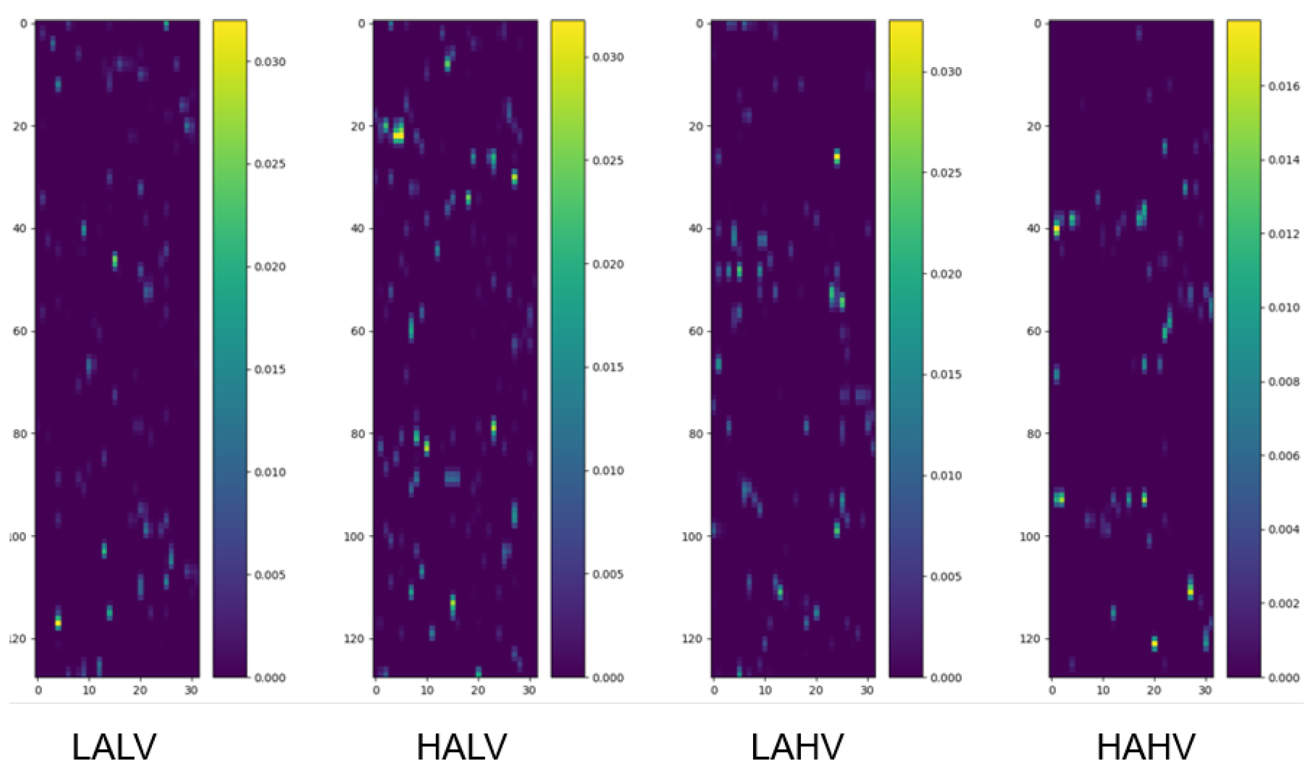
We randomly selected four samples from the pooled dataset (encompassing all participants) corresponding to the four categories under the quaternary classification task and drew their class activation maps, as shown in
Figure 2.
We randomly selected two samples from the pooled dataset (encompassing all participants) corresponding to the two categories under the binary classification task (Arousal and Valence, respectively) and drew their class activation maps, as shown in
Figure 3.
The results of the class activation maps indicate that different channels have different contributions to the classification results, and the prediction of classification results does not rely on all channels. Therefore, we use category activation thermal maps to screen out channels that contribute significantly to the classification results, optimize the model, reduce the number of electrodes in the data acquisition process, reduce the difficulty of signal acquisition, and improve the comfort of the signal acquisition process.
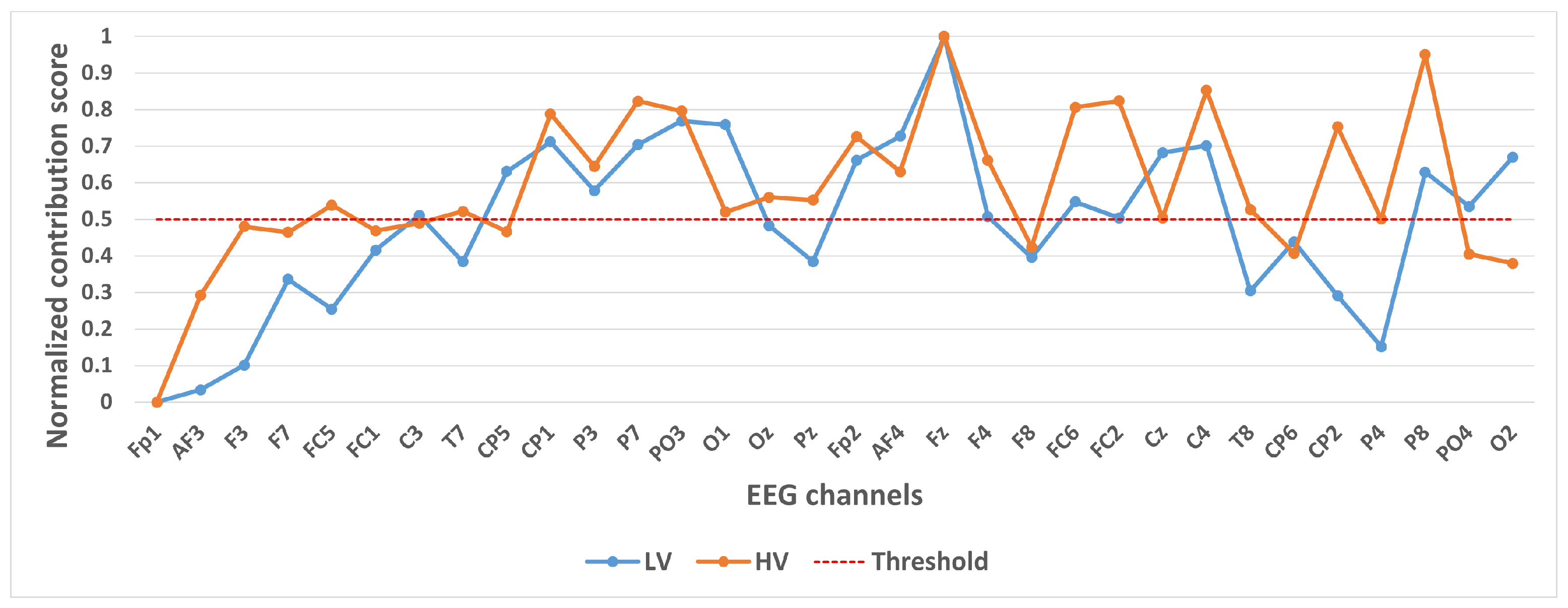
We took 14,000 samples under each category separately and plotted their category activation heat map. In order to analyze the contribution of different channels to the classification results, we take the mean value of each channel of the category activation heat map for each sample, and finally take the mean value of all the samples according to different categories and normalize them. These values were normalized to a 0–1 range to generate a Normalized Contribution Score, which reflects the relative importance of each channel in distinguishing emotional states. The results are shown in
Figure 4,
Figure 5 and
Figure 6. The y-axis in these figures is labeled “Normalized Contribution Score”, where higher values indicate greater influence of the corresponding channel on the model’s classification decisions. This normalization ensures consistency across categories and tasks, facilitating the direct comparison of channel importance across different emotional classification scenarios.
In selecting electrodes with significant contributions, the determination of thresholds was based on the distribution characteristics of channel contribution scores and the principle of spatial continuity of brain regions. For the quaternary classification task, the contribution values of the 32 channels showed a natural boundary at 0.5 (most low-contribution electrodes had values < 0.5, while most high-contribution electrodes had values > 0.5). Using 0.5 as the threshold retained 13 electrodes, covering continuous brain regions in the frontal and parietal lobes, and avoided the disruption of spatial continuity caused by excessively high thresholds (e.g., 0.6). For the binary Valence task, the 14 electrodes selected by the 0.5 threshold formed a complete “prefrontal-parietal” collaborative network, whereas increasing the threshold to 0.6 would break the connectivity of this network. For the binary Arousal task, high-contribution electrodes were highly concentrated in the central-parietal cluster. A threshold of 0.6 precisely retained 10 core electrodes, excluded low-contribution redundant channels (e.g., marginal electrodes with contribution values < 0.6), and maintained the spatial continuity of electrodes within the cluster. The above threshold selection balances the retention of key information and optimization of electrode quantity, which is consistent with the neurobiological mechanisms of emotional processing.
Figure 4 shows the contribution of different channels to the classification results under the quaternary classification task. It is easy to notice that 13 channels, CP5, CP1, P3, P7, PO3, O1, Oz, F4, F8, FC6, FC2, Cz, and C4, contribute more to the classification.
Figure 5 shows the contribution of different channels to the classification results under the binary classification task (Arousal). It is easy to notice that the 10 channels CP1, P3, P7, PO3, O1, Oz, Pz, F4, F8, FC6 contribute more to the classification.
Figure 6 shows the contribution of different channels to the classification results under the binary classification task (Valence). It is easy to notice that 14 channels, CP1, P3, P7, PO3, O1, Fp2, AF4, Fz, F4, FC6, FC2, Cz, C4, P8, contribute more to the classification.
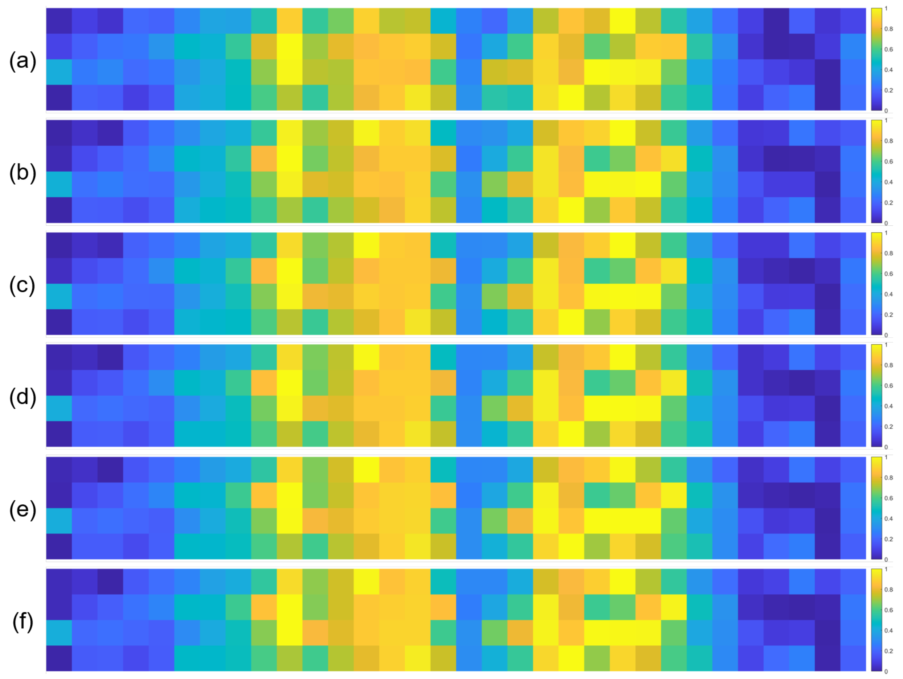
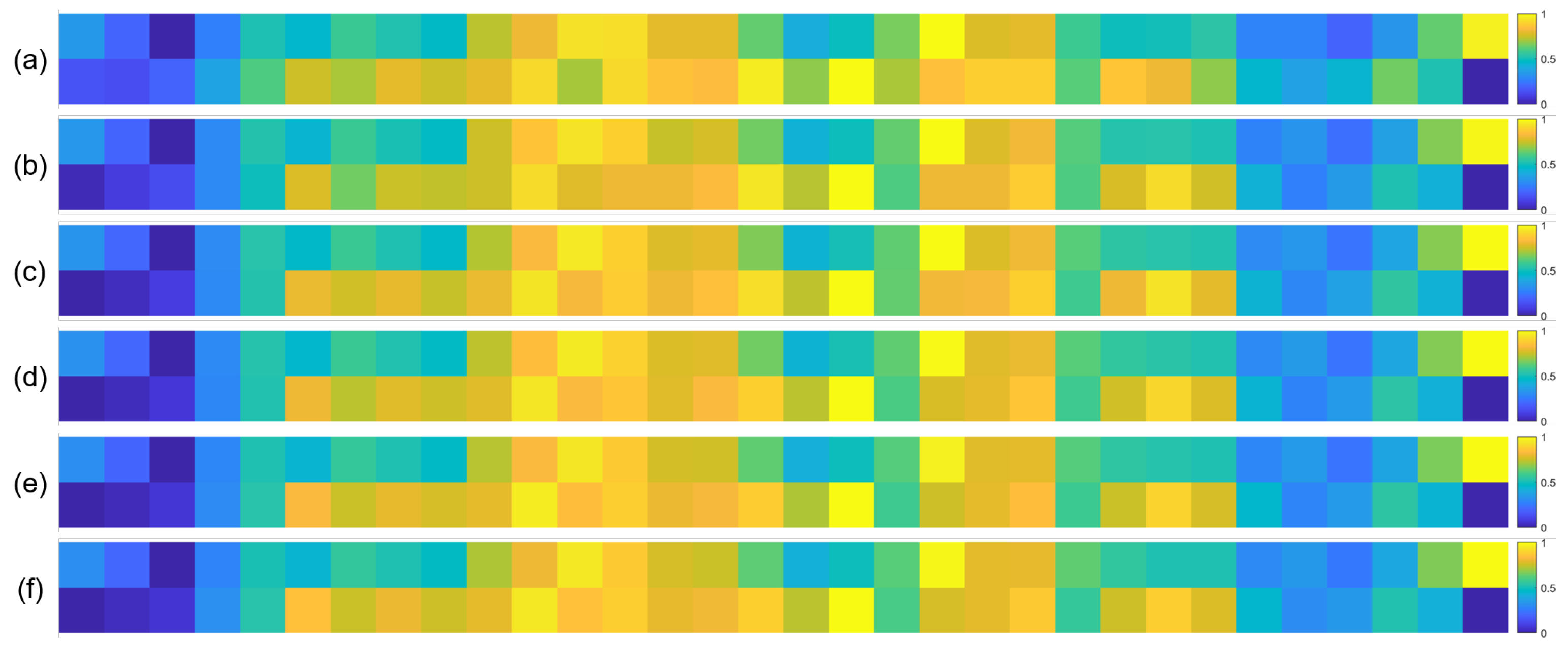
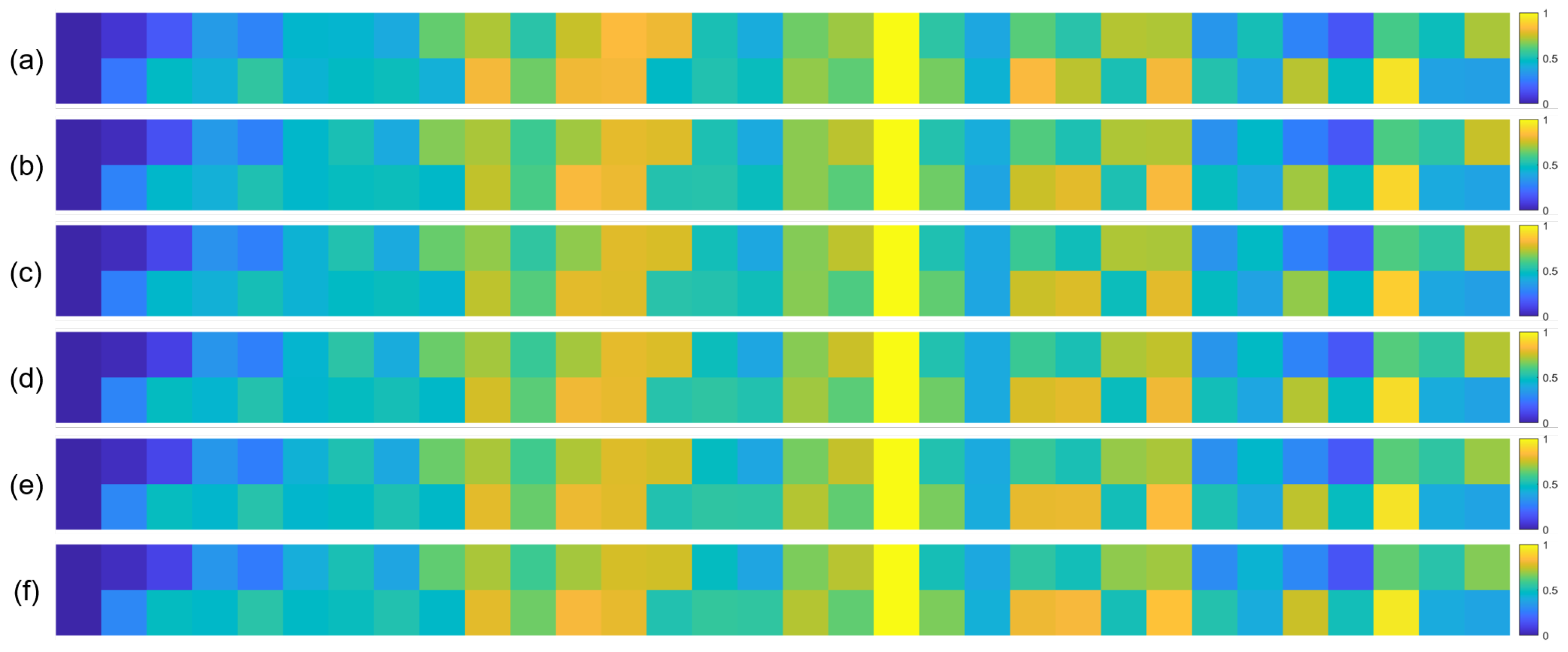
To further validate the robustness of the identified important EEG channels across varying sample sizes, we conducted a systematic analysis by randomly extracting subsets of 1000, 3000, 5000, 7000, and 10,000 samples from the full dataset (14,000 samples). For each subset, we recalculated the normalized contribution scores of the 32 EEG channels and visualized their distribution through heatmaps, with separate analyses performed for the quaternary classification task (
Figure 7), binary arousal classification (
Figure 8), and binary valence classification (
Figure 9).
A visual inspection of these heatmaps reveals striking consistency in the spatial patterns of channel contributions across all subset sizes. In each subplot, the warmer color clusters—indicating higher contribution—are concentrated in overlapping regions, regardless of sample size. For instance, in the quaternary classification task (
Figure 7), the right frontal channels (F4, F8, FC6) and left parietal channels (CP5, P3, P7) consistently exhibit elevated contributions across all subsets, mirroring the activation pattern observed in the full 14,000-sample dataset. This visual coherence directly supports the stability of the model’s interpretive focus, as the key channels driving classification decisions remain unchanged even when the sample size is reduced by nearly 93% (from 14,000 to 1000).
To quantify this consistency, we performed statistical analyses by comparing the channel contribution vectors of each subset with those of the full dataset, using Pearson correlation coefficients (PCC) as the metric. The results, summarized in
Table 4,
Table 5 and
Table 6, further confirm the robustness of our findings. In the quaternary task, all subsets achieved a PCC of 0.94 or higher, with most reaching a perfect correlation of 1.00, indicating near-identical contribution patterns. Similarly, the binary Arousal task yielded PCC values ranging from 0.87 to 1.00, while the valence task showed correlations between 0.81 and 1.00. These high correlation coefficients demonstrate that the relative importance of each channel is statistically consistent across different sample sizes.
Moreover, the tables explicitly list the high-contribution channels for each subset, revealing a remarkable overlap in the core set of electrodes. For example, in the valence classification task (
Table 6), channels such as CP1, P3, P7, and F4 appear in all subsets, with only minor variations in peripheral channels (e.g., occasional inclusion or exclusion of Oz or Cz). This consistency in the core channel set reinforces the conclusion that the model’s interpretive insights are not artifacts of specific data partitions but reflect genuine neurophysiological markers associated with emotion recognition.
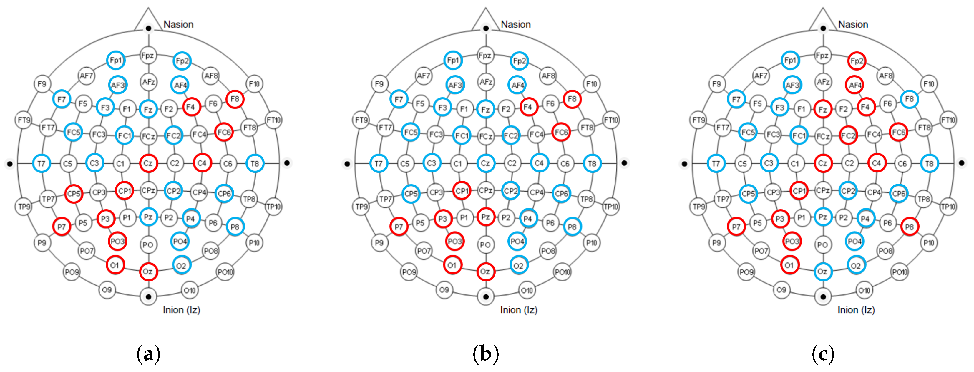
The International 10–20 System is an internationally recognized method for describing and applying the position of scalp electrodes in electroencephalography or polysomnography.
Figure 10 shows the electrodes used in the dataset collection process under the 10–20 system, and we mark the electrode positions that contribute significantly to the classification in red. It can be observed that in our proposed model, the electrodes that contribute significantly to classification are mainly distributed on the right side of the frontal lobe, the left side of the parietal lobe, and some intermediate regions. Furthermore, it showed similar results in all tasks. This result is consistent with biological discoveries [
16,
17].
3.3. Performance Comparison with Existing Models
For the two-class classification task, the proposed 2D-CNN model demonstrates superior performance, achieving 95.21% and 94.59% accuracy in arousal and valence classification, respectively.
Table 7 presents a comparative analysis of our model against previous studies, primarily evaluated using 10-fold cross-validation on the DEAP dataset.
Compared to traditional machine learning approaches, such as the HOS+LSTM method proposed by Sharma et al. [
1] and the EEG-GCN model by Gao et al. [
3], our model outperforms them by approximately 10% and 13% in arousal classification and 10.43% and 12.82% in valence classification, respectively. Similarly, the deep learning-based methods from Yin et al. [
2] and Cheng et al. [
6], which incorporate graph convolutional and transformer-based architectures, achieve high classification performance, but our approach surpasses them by notable margins, with improvements of 9.94% in arousal and up to 14.33% in valence classification.
When compared with advanced deep learning architectures, such as the EWT-3D-CNN-BiLSTM-GRU-AT model by Celebi et al. [
9] and the 2D-CNN-LSTM framework by Wang et al. [
7], our method still achieves higher accuracy, improving arousal classification by 4.62% and 3.31%, and valence classification by 4.02% and 2.29%, respectively. While the CADD-DCCNN model from Li et al. [
18] reaches competitive performance with 92.42% and 90.97% accuracy, our model still provides an advantage of approximately 2.79% and 3.62% in arousal and valence classification.
Table 7.
The comparison of our model with previous studies in the binary classification task.
Table 7.
The comparison of our model with previous studies in the binary classification task.
| Research | Method | Accuracy | % Below Our Model | Year |
|---|
|
Arousal
|
Valence
|
Arousal
|
Valence
|
|---|
| Sharma et al. [1] | HOS+LSTM | 85.21 | 84.16 | 10 | 10.43 | 2020 |
| Yin et al. [2] | GCNN-LSTM | 85.27 | 84.81 | 9.94 | 9.78 | 2021 |
| Gao et al. [3] | EEG-GCN | 81.95 | 81.77 | 13.26 | 12.82 | 2022 |
| Ghosh et al. [19] | Gradient Ascent | 88.67 | 86.95 | 6.54 | 7.64 | 2023 |
| Cheng et al. [6] | R2G-STLT | 86.22 | 80.26 | 8.99 | 14.33 | 2024 |
| Houssein et al. [8] | HcF+eCOA+MLPNN | 85.17 | 91.99 | 10.04 | 2.6 | 2024 |
| Celebi et al. [9] | EWT-3D-CNN-BiLSTM-GRU-AT | 90.59 | 90.57 | 4.62 | 4.02 | 2024 |
| Wang et al. [7] | 2D-CNN-LSTM | 91.9 | 92.3 | 3.31 | 2.29 | 2024 |
| Li et al. [18] | CADD-DCCNN | 92.42 | 90.97 | 2.79 | 3.62 | 2024 |
| Our Model | 2D-CNN | 95.21 | 94.59 | - | - | 2025 |
For the quaternary classification task, our 2D-CNN model achieves 93.01% accuracy on the DEAP dataset, outperforming previous approaches (
Table 8). Compared to traditional methods like Gupta et al. [
20] and Soroush et al. [
21], our model improves accuracy by over 21% and 11%, respectively. It also surpasses deep learning models such as those of Sharma et al. [
1] and Houssein et al. [
8], with gains of up to 11% and 3.48%.

