
EEG-Based Seizure Detection Using Dual-Branch CNN-ViT Network Integrating Phase and Power Spectrograms

 , and
, and
Abstract
1. Introduction
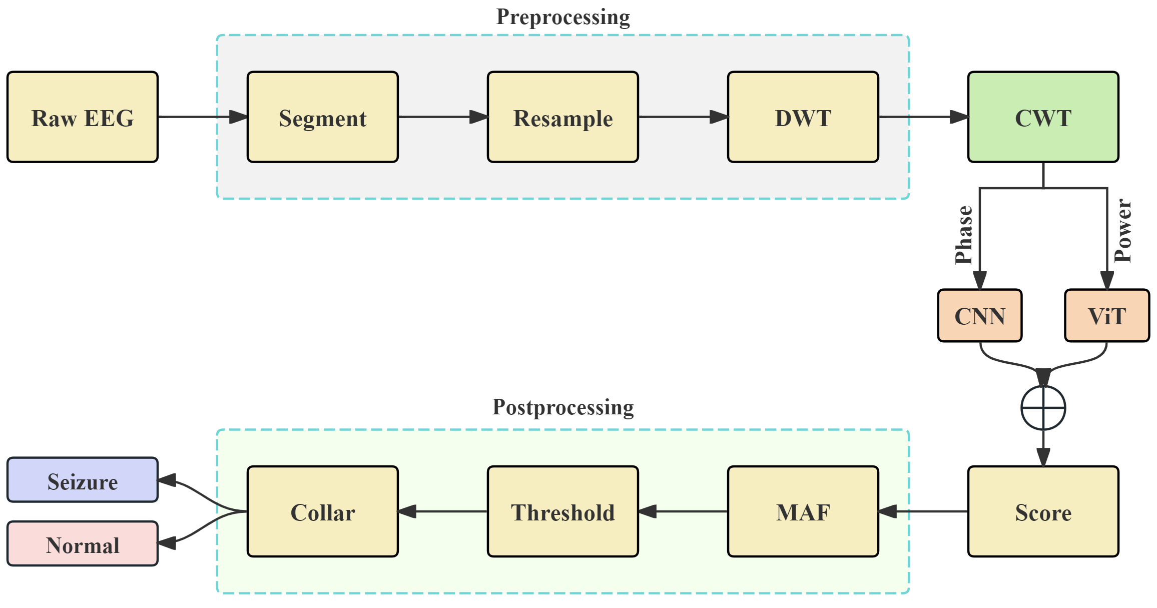
- We propose a dual-branch CNN-ViT hybrid network based on the phase and power spectrogram derived from CWT, enabling the complementary representation of time–frequency features and resulting in a significant improvement in seizure detection performance.
- We systematically reveal the sensitivity of CNN to the phase spectrogram and the modeling advantages of ViT for the power spectrogram, demonstrating the rationality of the network design.
- We evaluate the proposed network on the public CHB-MIT database and our clinically collected SH-SDU database. The proposed seizure detection framework demonstrates excellent performance in terms of sensitivity, specificity, and accuracy, showing its clinical generalization potential.
2. EEG Database
2.1. CHB-MIT Database
2.2. SH-SDU Database
3. Method
3.1. Preprocessing
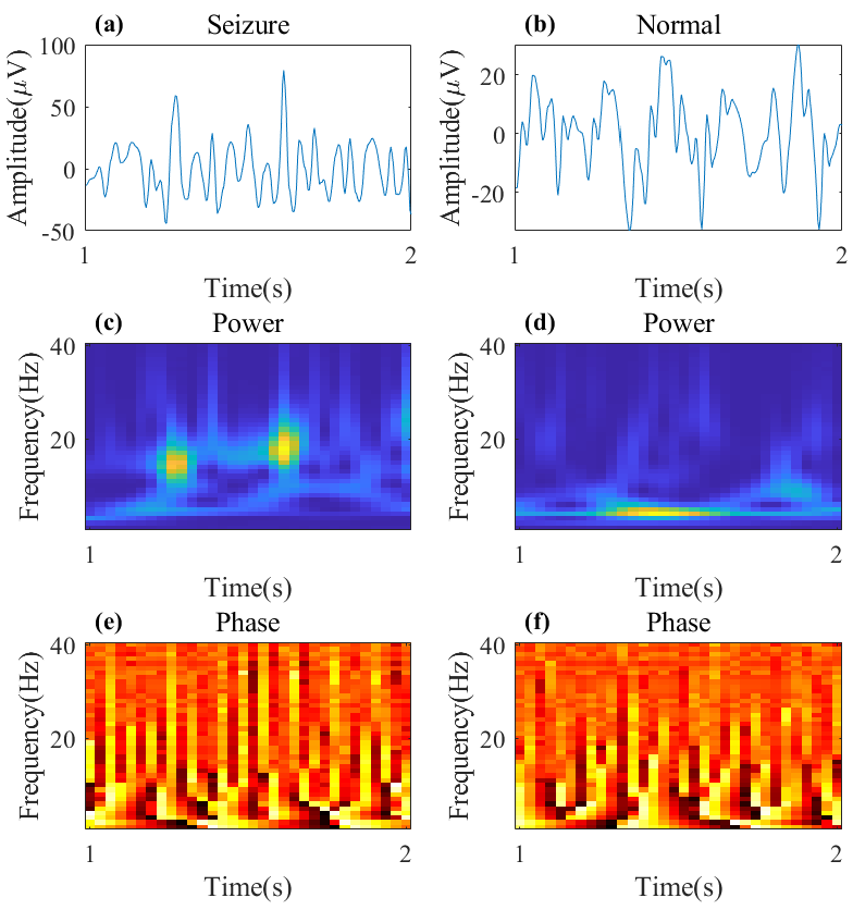
3.2. CWT with Complex Morlet Wavelet
3.3. Hybrid CNN-ViT Architecture for Seizure Detection
3.3.1. CNN with Shortcut Based on Phase Spectrogram
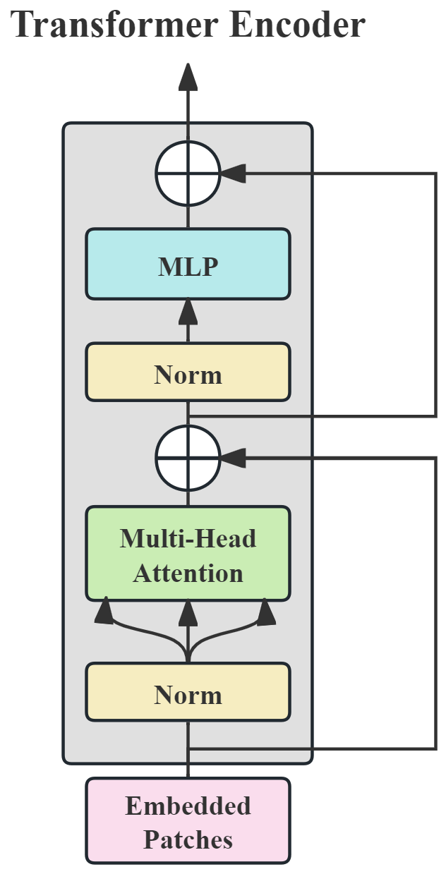
3.3.2. ViT Based on Power Spectrogram
3.4. Model Training
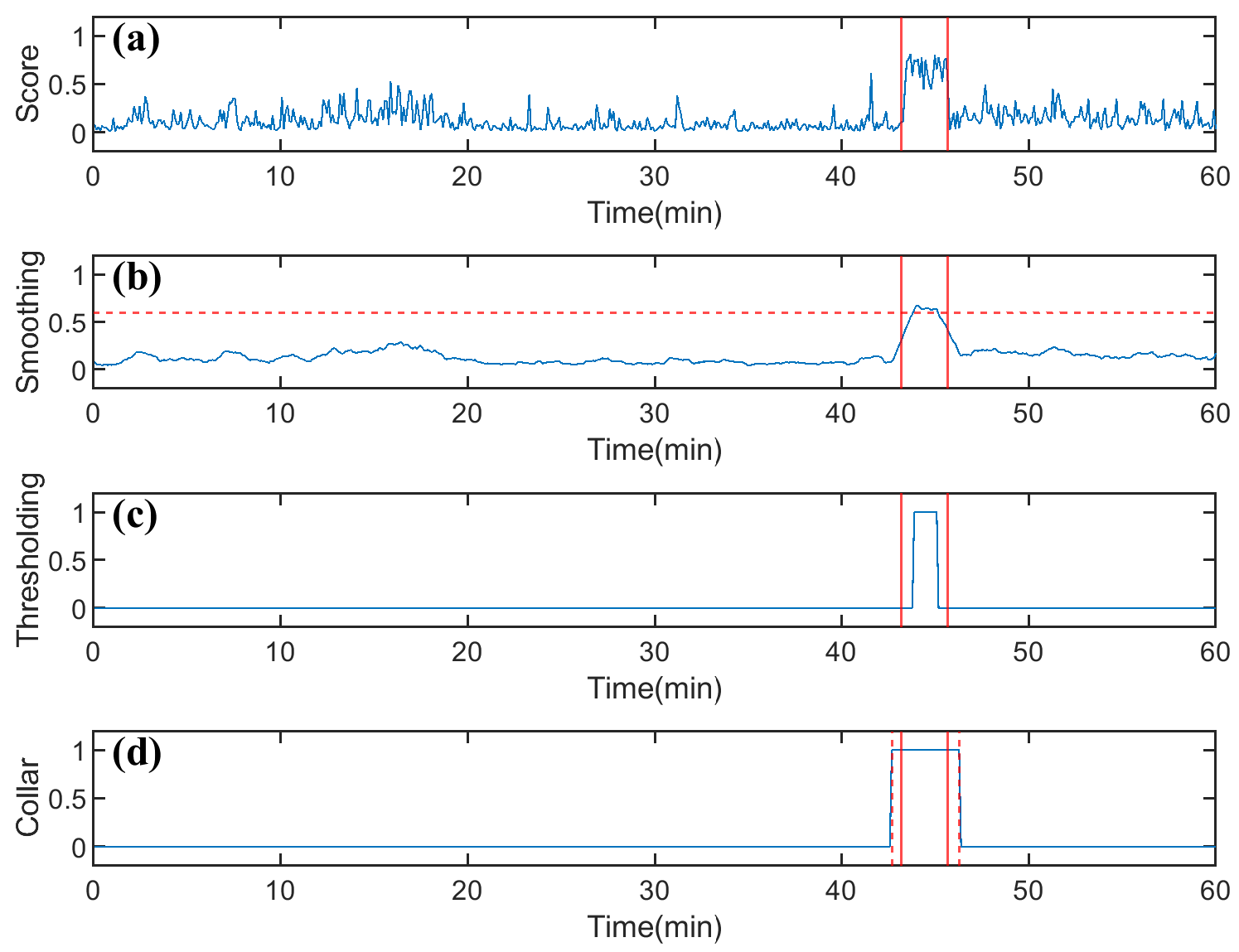
3.5. Postprocessing
3.6. Performance Metrics and Evaluation Setup
4. Results
4.1. Results on CHB-MIT Database
4.2. Result on SH-SDU Database
5. Discussion
5.1. Ablation Study
5.1.1. Effect of Network Structure
5.1.2. Effect of Time–Frequency Methods
5.1.3. Effect of CWT Wavelet Parameters
5.1.4. Effect of ViT Branch Depths
5.1.5. Effect of Threshold Settings
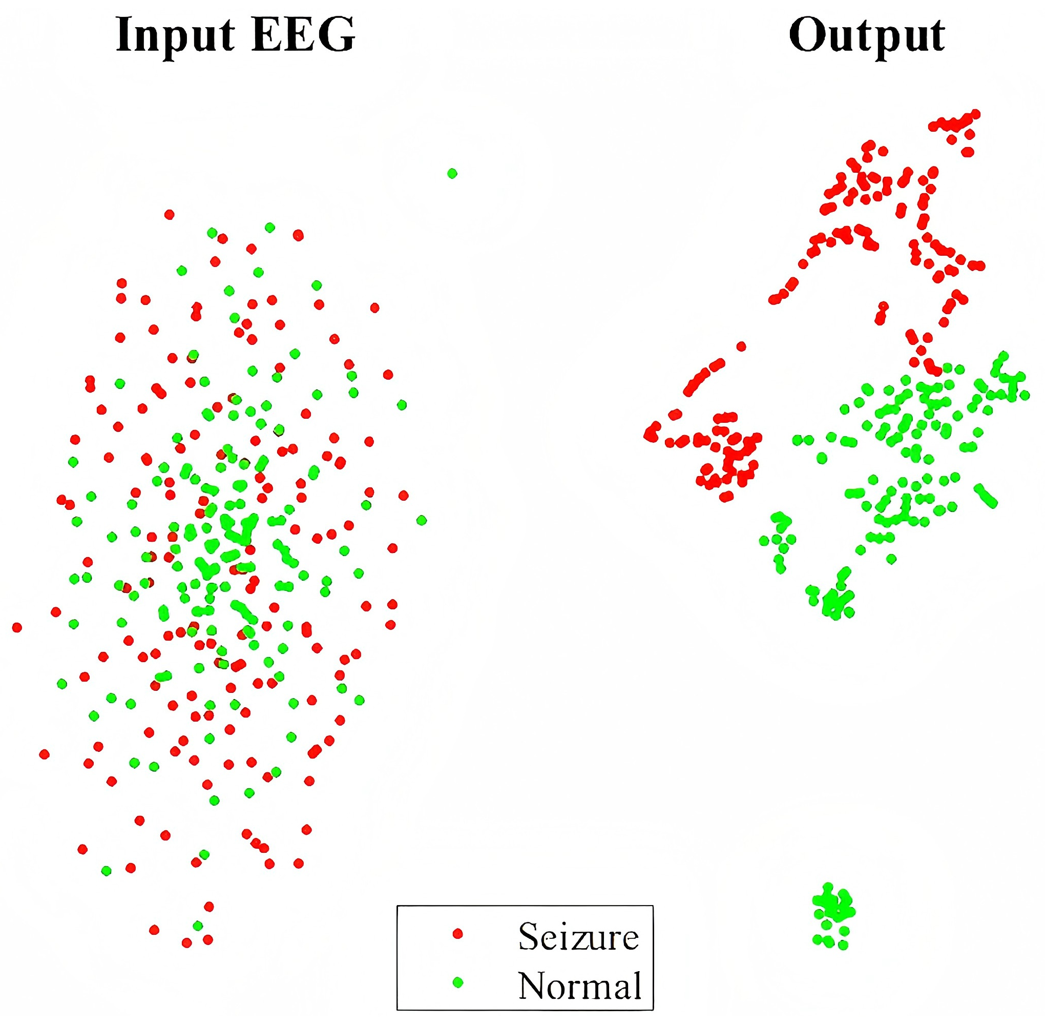
5.2. Visualization with t-SNE
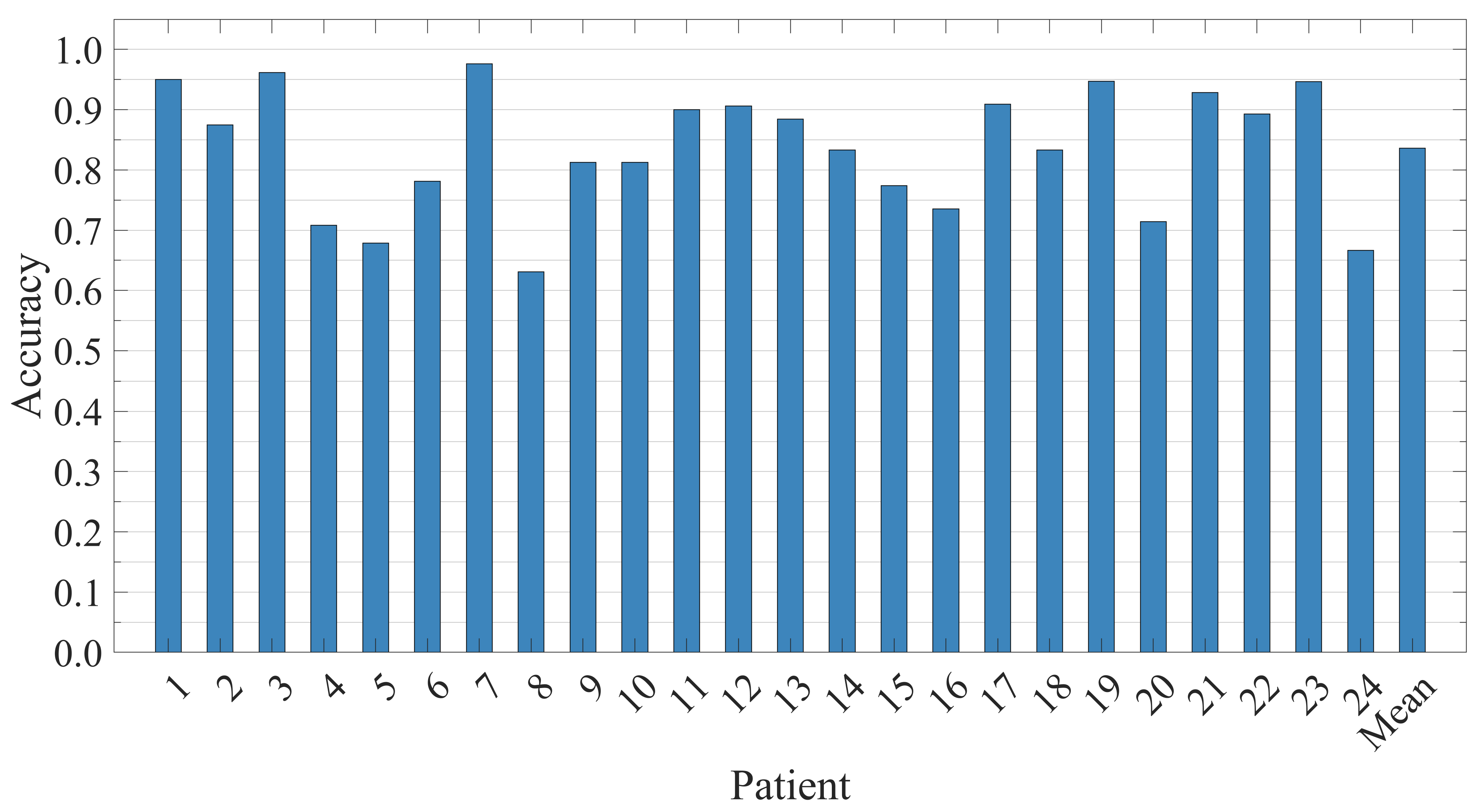
5.3. Patient-Independent Performance Evaluation
5.4. Compared with Existing Methods
6. Conclusions
Author Contributions
Funding
Institutional Review Board Statement
Informed Consent Statement
Data Availability Statement
Conflicts of Interest
References
- World Health Organization. Epilepsy. 2020. Available online: https://www.who.int/news-room/fact-sheets/detail/epilepsy (accessed on 7 July 2020).
- Fiest, K.M.; Sauro, K.M.; Wiebe, S.; Patten, S.B.; Kwon, C.S.; Dykeman, J.; Pringsheim, T.; Lorenzetti, D.L.; Jetté, N. Prevalence and incidence of epilepsy. Neurology 2017, 88, 296–303. [Google Scholar] [CrossRef]
- Bernhardt, B.C.; Worsley, K.J.; Besson, P.; Concha, L.; Lerch, J.P.; Evans, A.C.; Bernasconi, N. Mapping limbic network organization in temporal lobe epilepsy using morphometric correlations: Insights on the relation between mesiotemporal connectivity and cortical atrophy. NeuroImage 2008, 42, 515–524. [Google Scholar] [CrossRef]
- Kanner, A.M. Depression and epilepsy: A bidirectional relation? Epilepsia 2011, 52, 21–27. [Google Scholar] [CrossRef]
- Hesdorffer, D.C.; Ishihara, L.; Mynepalli, L.; Webb, D.J.; Weil, J.; Hauser, W.A. Epilepsy, suicidality, and psychiatric disorders: A bidirectional association. Ann. Neurol. 2012, 72, 184–191. [Google Scholar] [CrossRef] [PubMed]
- Whitney, R.; Sharma, S.; Jones, K.C.; RamachandranNair, R. Genetics and SUDEP: Challenges and Future Directions. Seizure Eur. J. Epilepsy 2023, 110, 188–193. [Google Scholar] [CrossRef]
- Gu, J.; Shao, W.; Liu, L.; Wang, Y.; Yang, Y.; Zhang, Z.; Wu, Y.; Xu, Q.; Gu, L.; Zhang, Y.; et al. Challenges and future directions of SUDEP models. Lab Anim 2024, 53, 226–243. [Google Scholar] [CrossRef]
- Tautan, A.M.; Andrei, A.G.; Smeralda, C.L.; Vatti, G.; Rossi, S.; Ionescu, B. Unsupervised learning from EEG data for epilepsy: A systematic literature review. Artif. Intell. Med. 2025, 162, 103095. [Google Scholar] [CrossRef] [PubMed]
- Glauser, T.A.; Cnaan, A.; Shinnar, S.; Hirtz, D.G.; Dlugos, D.; Masur, D.; Clark, P.O.; Capparelli, E.V.; Adamson, P.C. Ethosuximide, Valproic Acid, and Lamotrigine in Childhood Absence Epilepsy. N. Engl. J. Med. 2010, 362, 790–799. [Google Scholar] [CrossRef] [PubMed]
- Scheffer, I.E.; Berkovic, S.; Capovilla, G.; Connolly, M.B.; French, J.; Guilhoto, L.; Hirsch, E.; Jain, S.; Mathern, G.W.; Moshé, S.L.; et al. ILAE classification of the epilepsies: Position paper of the ILAE Commission for Classification and Terminology. Epilepsia 2017, 58, 512–521. [Google Scholar] [CrossRef]
- Noorlag, L.; Van Klink, N.E.; Kobayashi, K.; Gotman, J.; Braun, K.P.; Zijlmans, M. High-frequency oscillations in scalp EEG: A systematic review of methodological choices and clinical findings. Clin. Neurophysiol. 2022, 137, 46–58. [Google Scholar] [CrossRef]
- Jing, J.; Herlopian, A.; Karakis, I.; Ng, M.; Halford, J.J.; Lam, A.; Maus, D.; Chan, F.; Dolatshahi, M.; Muniz, C.F.; et al. Interrater Reliability of Experts in Identifying Interictal Epileptiform Discharges in Electroencephalograms. JAMA Neurol. 2020, 77, 49. [Google Scholar] [CrossRef]
- Gotman, J. Automatic recognition of epileptic seizures in the EEG. Electroencephalogr. Clin. Neurophysiol. 1982, 54, 530–540. [Google Scholar] [CrossRef]
- Zhou, W.; Liu, Y.; Yuan, Q.; Li, X. Epileptic Seizure Detection Using Lacunarity and Bayesian Linear Discriminant Analysis in Intracranial EEG. IEEE Trans. Biomed. Eng. 2013, 60, 3375–3381. [Google Scholar] [CrossRef] [PubMed]
- Kuhlmann, L.; Karoly, P.; Freestone, D.R.; Brinkmann, B.H.; Temko, A.; Barachant, A.; Li, F.; Titericz, G.; Lang, B.W.; Lavery, D.; et al. Epilepsyecosystem.org: Crowd-sourcing reproducible seizure prediction with long-term human intracranial EEG. Brain 2018, 141, 2619–2630. [Google Scholar] [CrossRef]
- Karoly, P.J.; Ung, H.; Grayden, D.B.; Kuhlmann, L.; Leyde, K.; Cook, M.J.; Freestone, D.R. The circadian profile of epilepsy improves seizure forecasting. Brain 2017, 140, 2169–2182. [Google Scholar] [CrossRef]
- Saggio, M.L.; Crisp, D.; Scott, J.M.; Karoly, P.; Kuhlmann, L.; Nakatani, M.; Murai, T.; Dümpelmann, M.; Schulze-Bonhage, A.; Ikeda, A.; et al. A taxonomy of seizure dynamotypes. eLife 2020, 9, e55632. [Google Scholar] [CrossRef] [PubMed]
- Shayeste, H.; Asl, B.M. Automatic seizure detection based on Gray Level Co-occurrence Matrix of STFT imaged-EEG. Biomed. Signal Process. Control. 2023, 79, 104109. [Google Scholar] [CrossRef]
- Shen, M.; Yang, F.; Wen, P.; Song, B.; Li, Y. A real-time epilepsy seizure detection approach based on EEG using short-time Fourier transform and Google-Net convolutional neural network. Heliyon 2024, 10, e31827. [Google Scholar] [CrossRef]
- Liu, G.; Zhou, W.; Geng, M. Automatic Seizure Detection Based on S-Transform and Deep Convolutional Neural Network. Int. J. Neur. Syst. 2020, 30, 1950024. [Google Scholar] [CrossRef]
- Liu, Y.; Liu, G.; Wu, S.; Tin, C. Phase spectrogram of EEG from S-transform Enhances epileptic seizure detection. Expert Syst. Appl. 2025, 262, 125621. [Google Scholar] [CrossRef]
- Ozdemir, M.A.; Cura, O.K.; Akan, A. Epileptic EEG Classification by Using Time-Frequency Images for Deep Learning. Int. J. Neur. Syst. 2021, 31, 2150026. [Google Scholar] [CrossRef] [PubMed]
- Cura, O.K.; Akan, A. Classification of Epileptic EEG Signals Using Synchrosqueezing Transform and Machine Learning. Int. J. Neur. Syst. 2021, 31, 2150005. [Google Scholar] [CrossRef] [PubMed]
- Leon, C. Time-Frequency Analysis: Theory and Applications; Pnentice Hall: Upper Saddle River, NJ, USA, 1995. [Google Scholar]
- Grossmann, A.; Morlet, J. Decomposition of Hardy Functions into Square Integrable Wavelets of Constant Shape. SIAM J. Math. Anal. 1984, 15, 723–736. [Google Scholar] [CrossRef]
- Mallat, S. A Wavelet Tour of Signal Processing; Elsevier: Amsterdam, The Netherlands, 1999. [Google Scholar]
- Jiang, G.; Wang, J.; Wang, L.; Xie, P.; Li, Y.; Li, X. An interpretable convolutional neural network with multi-wavelet kernel fusion for intelligent fault diagnosis. J. Manuf. Syst. 2023, 70, 18–30. [Google Scholar] [CrossRef]
- Park, H.S.; Yoo, S.H.; Oh, B.K. A dynamic strain prediction method for malfunction of sensors in buildings subjected to seismic loads using CWT and CNN. Sci. Rep. 2024, 14, 28156. [Google Scholar] [CrossRef] [PubMed]
- Fu, G. A robust bearing fault diagnosis method based on ensemble learning with adaptive weight selection. Expert Syst. Appl. 2025, 269, 126420. [Google Scholar] [CrossRef]
- Vaswani, A.; Shazeer, N.; Parmar, N.; Uszkoreit, J.; Jones, L.; Gomez, A.N.; Kaiser, L.; Polosukhin, I. Attention Is All You Need. arXiv 2023, arXiv:1706.03762. [Google Scholar] [CrossRef]
- Dosovitskiy, A.; Beyer, L.; Kolesnikov, A.; Weissenborn, D.; Zhai, X.; Unterthiner, T.; Dehghani, M.; Minderer, M.; Heigold, G.; Gelly, S.; et al. An Image is Worth 16x16 Words: Transformers for Image Recognition at Scale. arXiv 2021, arXiv:2010.11929. [Google Scholar]
- Krizhevsky, A.; Sutskever, I.; Hinton, G.E. ImageNet classification with deep convolutional neural networks. Commun. ACM 2017, 60, 84–90. [Google Scholar] [CrossRef]
- Ronneberger, O.; Fischer, P.; Brox, T. U-Net: Convolutional Networks for Biomedical Image Segmentation. arXiv 2015, arXiv:1505.04597. [Google Scholar] [CrossRef]
- Zhu, Z.; Wang, Z.; Qi, G.; Mazur, N.; Yang, P.; Liu, Y. Brain tumor segmentation in MRI with multi-modality spatial information enhancement and boundary shape correction. Pattern Recognit. 2024, 153, 110553. [Google Scholar] [CrossRef]
- Shoeb, A.H. Application of machine learning to epileptic seizure onset detection and treatment. Ph.D. Thesis, Massachusetts Institute of Technology, Cambridge, MA, USA, 2009. [Google Scholar]
- Faust, O.; Acharya, U.R.; Adeli, H.; Adeli, A. Wavelet-based EEG processing for computer-aided seizure detection and epilepsy diagnosis. Seizure 2015, 26, 56–64. [Google Scholar] [CrossRef] [PubMed]
- Fıçıcı, C.; Telatar, Z.; Eroğul, O. Automated temporal lobe epilepsy and psychogenic nonepileptic seizure patient discrimination from multichannel EEG recordings using DWT based analysis. Biomed. Signal Process. Control. 2022, 77, 103755. [Google Scholar] [CrossRef]
- Dissanayake, T.; Fernando, T.; Denman, S.; Sridharan, S.; Fookes, C. Patient-independent Epileptic Seizure Prediction using Deep Learning Models. arXiv 2020, arXiv:2011.09581. [Google Scholar] [CrossRef]
- Torrence, C.; Compo, G.P. A Practical Guide to Wavelet Analysis. Bull. Amer. Meteor. Soc. 1998, 79, 61–78. [Google Scholar] [CrossRef]
- Srivastava, N.; Hinton, G.; Krizhevsky, A.; Sutskever, I.; Salakhutdinov, R. Dropout: A Simple Way to Prevent Neural Networks from Overfitting. JMLR 2014, 15, 1929–1958. [Google Scholar]
- Hendrycks, D.; Gimpel, K. Gaussian Error Linear Units (GELUs). arXiv 2023, arXiv:1606.08415. [Google Scholar] [CrossRef]
- Ba, J.L.; Kiros, J.R.; Hinton, G.E. Layer Normalization. arXiv 2016, arXiv:1607.06450. [Google Scholar] [CrossRef]
- Kingma, D.P.; Ba, J. Adam: A Method for Stochastic Optimization. arXiv 2017, arXiv:1412.6980. [Google Scholar] [CrossRef]
- Smith, L.N. Cyclical Learning Rates for Training Neural Networks. In Proceedings of the 2017 IEEE Winter Conference on Applications of Computer Vision (WACV), Santa Rosa, CA, USA, 24–31 March 2017; pp. 464–472. [Google Scholar] [CrossRef]
- Masters, D.; Luschi, C. Revisiting Small Batch Training for Deep Neural Networks. arXiv 2018, arXiv:1804.07612. [Google Scholar] [CrossRef]
- Temko, A.; Thomas, E.; Marnane, W.; Lightbody, G.; Boylan, G. EEG-based neonatal seizure detection with Support Vector Machines. Clin. Neurophysiol. 2011, 122, 464–473. [Google Scholar] [CrossRef]
- Hanley, J.A.; McNeil, B.J. The meaning and use of the area under a receiver operating characteristic (ROC) curve. Radiology 1982, 143, 29–36. [Google Scholar] [CrossRef] [PubMed]
- Bradley, A.P. The use of the area under the ROC curve in the evaluation of machine learning algorithms. Pattern Recognit. 1997, 30, 1145–1159. [Google Scholar] [CrossRef]
- Stam, C.J.; Nolte, G.; Daffertshofer, A. Phase lag index: Assessment of functional connectivity from multi channel EEG and MEG with diminished bias from common sources. Hum. Brain Mapp. 2007, 28, 1178–1193. [Google Scholar] [CrossRef] [PubMed]
- Subasi, A. EEG signal classification using wavelet feature extraction and a mixture of expert model. Expert Syst. Appl. 2007, 32, 1084–1093. [Google Scholar] [CrossRef]
- Stockwell, R. Why use the S-transform. Pseudo-Differ. Oper. Partial. Differ. Equ.-Time-Freq. Anal. 2007, 52, 279–309. [Google Scholar]
- Zhang, Z.G.; Hung, Y.S.; Chan, S.C. Local Polynomial Modeling of Time-Varying Autoregressive Models with Application to Time–Frequency Analysis of Event-Related EEG. IEEE Trans. Biomed. Eng. 2011, 58, 557–566. [Google Scholar] [CrossRef]
- Teolis, A. Computational Signal Processing with Wavelets, 1st ed.; Birkhäuser Basel: Basel, Switzerland, 2012. [Google Scholar]
- van der Maaten, L.; Hinton, G.E. Visualizing Data using t-SNE. J. Mach. Learn. Res. 2008, 9, 2579–2605. [Google Scholar]
- Li, C.; Zhou, W.; Liu, G.; Zhang, Y.; Geng, M.; Liu, Z.; Wang, S.; Shang, W. Seizure Onset Detection Using Empirical Mode Decomposition and Common Spatial Pattern. IEEE Trans. Neural Syst. Rehabil. Eng. 2021, 29, 458–467. [Google Scholar] [CrossRef]
- Cimr, D.; Fujita, H.; Tomaskova, H.; Cimler, R.; Selamat, A. Automatic seizure detection by convolutional neural networks with computational complexity analysis. Comput. Methods Programs Biomed. 2023, 229, 107277. [Google Scholar] [CrossRef]
- Zhao, Y.; Chu, D.; He, J.; Xue, M.; Jia, W.; Xu, F.; Zheng, Y. Interactive local and global feature coupling for EEG-based epileptic seizure detection. Biomed. Signal Process. Control. 2023, 81, 104441. [Google Scholar] [CrossRef]
- Liu, C.; Chen, W.; Zhang, T. Wavelet-Hilbert transform based bidirectional least squares grey transform and modified binary grey wolf optimization for the identification of epileptic EEGs. Biocybern. Biomed. Eng. 2023, 43, 442–462. [Google Scholar] [CrossRef]
- Liu, G.; Tian, L.; Wen, Y.; Yu, W.; Zhou, W. Cosine convolutional neural network and its application for seizure detection. Neural Netw. 2024, 174, 106267. [Google Scholar] [CrossRef]
- Li, H. End-to-end model for automatic seizure detection using supervised contrastive learning. Eng. Appl. Artif. Intell. 2024, 13, 108665. [Google Scholar] [CrossRef]
- Cao, X.; Zheng, S.; Zhang, J.; Chen, W.; Du, G. A hybrid CNN-Bi-LSTM model with feature fusion for accurate epilepsy seizure detection. BMC Med. Inform. Decis. Mak. 2025, 25, 6. [Google Scholar] [CrossRef] [PubMed]


| Patient–Sex–Age | Seizure Type | Seizure Onset Zone | Total Duration (h) | Mean Seizure Duration (s) | Training Seizure Duration (min) | Training Non-Seizure Duration (min) | Testing EEG Duration (h) |
|---|---|---|---|---|---|---|---|
| 1-F-11 | SP, CP | Temporal | 40.55 | 63.15 | 0.67 | 3.33 | 40.48 |
| 2-M-11 | SP, CP, GTC | Frontal | 35.27 | 57.34 | 1.35 | 6.75 | 35.13 |
| 3-F-14 | SP, CP | Temporal | 38.00 | 57.43 | 0.87 | 4.33 | 37.91 |
| 4-M-22 | SP, CP, GTC | Temporal, Occipital | 156.07 | 94.50 | 0.82 | 4.08 | 155.99 |
| 5-F-7 | CP, GTC | Frontal | 39.00 | 111.60 | 1.92 | 9.58 | 38.81 |
| 6-F-1.5 | CP, GTC | Temporal | 66.74 | 15.30 | 1.07 | 5.33 | 66.63 |
| 7-F-14.5 | SP, CP, GTC | Temporal | 67.05 | 108.34 | 1.43 | 7.17 | 66.91 |
| 8-M-3.5 | SP, CP, GTC | Temporal | 20.01 | 183.80 | 2.85 | 14.25 | 19.72 |
| 9-F-10 | CP, GTC | Frontal | 67.87 | 69.00 | 1.07 | 5.33 | 67.76 |
| 10-M-3 | SP, CP, GTC | Temporal | 50.02 | 65.50 | 0.58 | 2.92 | 49.96 |
| 11-F-12 | SP, CP, GTC | Frontal | 34.79 | 268.67 | 0.37 | 1.83 | 34.75 |
| 12-F-2 | SP, CP, GTC | Frontal | 20.69 | 36.63 | 2.15 | 10.75 | 20.47 |
| 13-F-3 | SP, CP, GTC | Temporal, Occipital | 33.00 | 44.59 | 3.48 | 17.42 | 32.65 |
| 14-F-9 | CP, GTC | Temporal | 26.00 | 21.13 | 0.23 | 1.17 | 25.98 |
| 15-M-16 | SP, CP, GTC | Frontal, Temporal | 40.01 | 99.60 | 2.08 | 10.42 | 39.80 |
| 16-F-7 | SP, CP, GTC | Temporal | 19.00 | 8.40 | 1.15 | 5.75 | 18.88 |
| 17-F-12 | SP, CP, GTC | Temporal | 21.01 | 97.67 | 1.50 | 7.50 | 20.86 |
| 18-F-18 | SP, CP | Temporal, Occipital | 35.63 | 52.84 | 0.83 | 4.17 | 35.55 |
| 19-F-19 | SP, CP, GTC | Frontal | 29.93 | 78.67 | 1.30 | 6.50 | 29.80 |
| 20-F-6 | SP, CP, GTC | Temporal | 27.60 | 36.75 | 0.48 | 2.42 | 27.55 |
| 21-F-13 | SP, CP | Temporal | 32.83 | 49.75 | 0.93 | 4.67 | 32.74 |
| 22-F-9 | - | Temporal, Occipital | 31.00 | 68.00 | 0.97 | 4.83 | 30.90 |
| 23-F-6 | - | Frontal | 26.56 | 60.58 | 1.88 | 9.42 | 26.37 |
| 24-/-/ | - | - | 21.30 | 31.94 | 0.42 | 2.08 | 21.26 |
| Summary | - | - | 979.93 | - | 30.40 | 152.02 | 976.89 |
| Patient–Sex–Age | Seizure Type | Seizure Onset Zone | Total Duration (h) | Mean Seizure Duration (s) | Number of Used Seizures |
|---|---|---|---|---|---|
| 1-F-28 | CP | Temporal, Frontal | 20.58 | 40.53 | 19–17 |
| 2-M-61 | CP | Central, Temporal | 16.04 | 220.80 | 10–8 |
| 3-M-34 | CP | Temporal, Frontal | 12.00 | 52.20 | 10–8 |
| 4-M-72 | CP | Temporal, Frontal | 15.56 | 109.38 | 29–27 |
| 5-M-79 | SP | Parietal, Occipital | 17.37 | 68.71 | 38–35 |
| 6-F-38 | SP | Temporal | 6.00 | 34.67 | 3–2 |
| Summary | - | - | 87.55 | - | 109–97 |
| Patient | Sensitivity | Specificity | Accuracy |
|---|---|---|---|
| 1 | 100.00% | 99.79% | 99.86% |
| 2 | 100.00% | 99.96% | 99.97% |
| 3 | 100.00% | 99.66% | 99.78% |
| 4 | 82.56% | 97.73% | 95.58% |
| 5 | 100.00% | 99.89% | 99.93% |
| 6 | 100.00% | 99.88% | 99.92% |
| 7 | 96.72% | 99.40% | 99.05% |
| 8 | 100.00% | 80.13% | 86.76% |
| 9 | 100.00% | 99.95% | 99.97% |
| 10 | 100.00% | 99.94% | 99.96% |
| 11 | 100.00% | 99.80% | 99.87% |
| 12 | 91.77% | 98.16% | 97.41% |
| 13 | 87.78% | 96.93% | 95.92% |
| 14 | 100.00% | 95.57% | 97.04% |
| 15 | 95.26% | 97.94% | 96.96% |
| 16 | 100.00% | 99.81% | 99.87% |
| 17 | 100.00% | 99.89% | 99.93% |
| 18 | 100.00% | 99.01% | 99.34% |
| 19 | 100.00% | 99.14% | 99.43% |
| 20 | 100.00% | 99.20% | 99.46% |
| 21 | 100.00% | 99.85% | 99.90% |
| 22 | 100.00% | 99.99% | 99.99% |
| 23 | 100.00% | 98.31% | 98.87% |
| 24 | 100.00% | 97.13% | 98.12% |
| Average | 98.09% | 98.21% | 98.45% |
| Patient | Number of Expert- Marked Seizures | Number of Detected Seizures | Sensitivity | FDR (/h) | Latency (s) |
|---|---|---|---|---|---|
| 1 | 6 | 6 | 100.00% | 0.0247 | −15.43 |
| 2 | 2 | 2 | 100.00% | 0.0284 | −1.33 |
| 3 | 6 | 6 | 100.00% | 0.0790 | −9.71 |
| 4 | 3 | 3 | 100.00% | 0.2884 | −33.00 |
| 5 | 4 | 4 | 100.00% | 0.0257 | −24.00 |
| 6 | 6 | 6 | 100.00% | 0.2398 | −1.60 |
| 7 | 2 | 2 | 100.00% | 0.0895 | −82.67 |
| 8 | 4 | 4 | 100.00% | 0.0501 | −24.00 |
| 9 | 3 | 3 | 100.00% | 0.0147 | −9.00 |
| 10 | 5 | 5 | 100.00% | 0.0400 | −9.33 |
| 11 | 2 | 2 | 100.00% | 0.0287 | −49.33 |
| 12 | 23 | 23 | 100.00% | 0.7103 | −9.93 |
| 13 | 8 | 8 | 100.00% | 1.2144 | −20.67 |
| 14 | 7 | 7 | 100.00% | 1.8080 | −28.50 |
| 15 | 19 | 18 | 94.74% | 0.5003 | −27.37 |
| 16 | 2 | 2 | 100.00% | 0.4744 | −3.50 |
| 17 | 2 | 2 | 100.00% | 0.0477 | −14.67 |
| 18 | 5 | 4 | 80.00% | 0.3369 | −21.33 |
| 19 | 2 | 2 | 100.00% | 0.1003 | −14.67 |
| 20 | 7 | 7 | 100.00% | 0.3262 | −13.00 |
| 21 | 3 | 3 | 100.00% | 0.0914 | −4.00 |
| 22 | 2 | 2 | 100.00% | 0 | −40.00 |
| 23 | 6 | 6 | 100.00% | 0.5278 | −16.00 |
| 24 | 15 | 15 | 100.00% | 0.2819 | −47.25 |
| Average | 144 | 142 | 98.95% | 0.3054 | −21.68 |
| Patient | Sensitivity | Specificity | Accuracy |
|---|---|---|---|
| 1 | 79.28% | 94.04% | 90.61% |
| 2 | 88.80% | 97.83% | 96.69% |
| 3 | 99.12% | 98.17% | 98.63% |
| 4 | 79.53% | 90.50% | 90.26% |
| 5 | 87.38% | 92.24% | 91.77% |
| 6 | 100.00% | 100.00% | 100.00% |
| Average | 89.02% | 95.46% | 94.66% |
| Patient | Number of Expert-Marked Seizures | Number of Detected Seizures | Sensitivity | FDR (/h) | Latency (s) |
|---|---|---|---|---|---|
| 1 | 17 | 15 | 88.24% | 3.8416 | −13.88 |
| 2 | 8 | 8 | 100.00% | 0.3137 | −8 |
| 3 | 8 | 8 | 100.00% | 2.0046 | −7.6 |
| 4 | 27 | 27 | 100.00% | 2.7089 | −16.97 |
| 5 | 35 | 33 | 94.29% | 3.8731 | −8.56 |
| 6 | 2 | 2 | 100.00% | 0 | 0 |
| Average | 97 | 93 | 97.09% | 2.1237 | −9.17 |
| Model | AUC | FDR(/h) | Accuracy |
|---|---|---|---|
| CNN based on power | 91.07% | 5.5373 | 93.63% |
| ViT based on power | 91.37% | 1.8081 | 97.30% |
| CNN based on phase | 80.49% | 5.8279 | 92.27% |
| ViT based on phase | 59.02% | 20.9708 | 75.16% |
| Hybrid | 92.57% | 0.7103 | 97.41% |
| AUC | Accuracy | |
|---|---|---|
| CWT | 92.57% | 97.41% |
| S-Transform | 89.46% | 95.37% |
| STFT | 90.18% | 96.21% |
| – | AUC | FDR |
|---|---|---|
| 1–0.5 | 92.56% | 1.2108 |
| 1–2 | 91.44% | 1.1139 |
| 1–4 | 91.69% | 0.8233 |
| 0.5–1 | 92.20% | 1.0171 |
| 2–1 | 91.79% | 1.0655 |
| 4–1 | 91.73% | 1.1139 |
| 1–1 | 92.57% | 0.7103 |
| Networks | Number of Parameters | AUC | FDR (/h) |
|---|---|---|---|
| CNN+1ViT | 249.8 k | 92.26% | 0.7104 |
| CNN+2ViT | 300.0 k | 93.13% | 0.8072 |
| CNN+3ViT | 350.1 k | 93.05% | 0.7587 |
| Author | Year | Feature Extraction Method | Classifier | Sensitivity | Specificity | Accuracy | FDR(/h) |
|---|---|---|---|---|---|---|---|
| Li et al. [55] | 2021 | EMD+CSP | SVM | 97.34% | 97.50% | - | 0.63 |
| Cimr et al. [56] | 2022 | Normalization | CNN | 97.06% | 99.27% | 96.99% | - |
| Zhao et al. [57] | 2023 | None | CNN+Transformer | 97.70% | 97.60% | 98.76% | - |
| Liu et al. [58] | 2023 | WPT+HTBiLGST | MBGWO+FKNN | 97.30% | 99.48% | 99.48% | - |
| Liu et al. [59] | 2024 | None | CosCNN | 98.12% | 99.31% | - | 0.69 |
| Li et al. [60] | 2024 | None | CNN-BiLSTM+Contrastive Loss | 98.97% | 97.36% | 97.36% | 0.35 |
| Cao et al. [61] | 2025 | Time-domain+Nonlinear Features | SVM-REF+CNN-BiLSTM | 97.84% | 99.21% | 98.43% | - |
| Our work | 2025 | CWT | CNN+ViT | 98.09% | 98.21% | 98.45% | 0.31 |
Disclaimer/Publisher’s Note: The statements, opinions and data contained in all publications are solely those of the individual author(s) and contributor(s) and not of MDPI and/or the editor(s). MDPI and/or the editor(s) disclaim responsibility for any injury to people or property resulting from any ideas, methods, instructions or products referred to in the content. |
© 2025 by the authors. Licensee MDPI, Basel, Switzerland. This article is an open access article distributed under the terms and conditions of the Creative Commons Attribution (CC BY) license (https://creativecommons.org/licenses/by/4.0/).
Share and Cite
Wang, Z.; Hu, Y.; Xin, Q.; Jin, G.; Zhao, Y.; Zhou, W.; Liu, G. EEG-Based Seizure Detection Using Dual-Branch CNN-ViT Network Integrating Phase and Power Spectrograms. Brain Sci. 2025, 15, 509. https://doi.org/10.3390/brainsci15050509
Wang Z, Hu Y, Xin Q, Jin G, Zhao Y, Zhou W, Liu G. EEG-Based Seizure Detection Using Dual-Branch CNN-ViT Network Integrating Phase and Power Spectrograms. Brain Sciences. 2025; 15(5):509. https://doi.org/10.3390/brainsci15050509
Chicago/Turabian StyleWang, Zhuohan, Yaoqi Hu, Qingyue Xin, Guanghao Jin, Yazhou Zhao, Weidong Zhou, and Guoyang Liu. 2025. "EEG-Based Seizure Detection Using Dual-Branch CNN-ViT Network Integrating Phase and Power Spectrograms" Brain Sciences 15, no. 5: 509. https://doi.org/10.3390/brainsci15050509
APA StyleWang, Z., Hu, Y., Xin, Q., Jin, G., Zhao, Y., Zhou, W., & Liu, G. (2025). EEG-Based Seizure Detection Using Dual-Branch CNN-ViT Network Integrating Phase and Power Spectrograms. Brain Sciences, 15(5), 509. https://doi.org/10.3390/brainsci15050509