
OViTAD: Optimized Vision Transformer to Predict Various Stages of Alzheimer’s Disease Using Resting-State fMRI and Structural MRI Data
 , ,
, ,
Abstract
1. Introduction
2. Related Work
3. Materials and Methods
3.1. Datasets
3.2. Image Acquisition Protocol
3.3. Data Preprocessing
3.3.1. rs-fMRI
3.3.2. Structural MRI
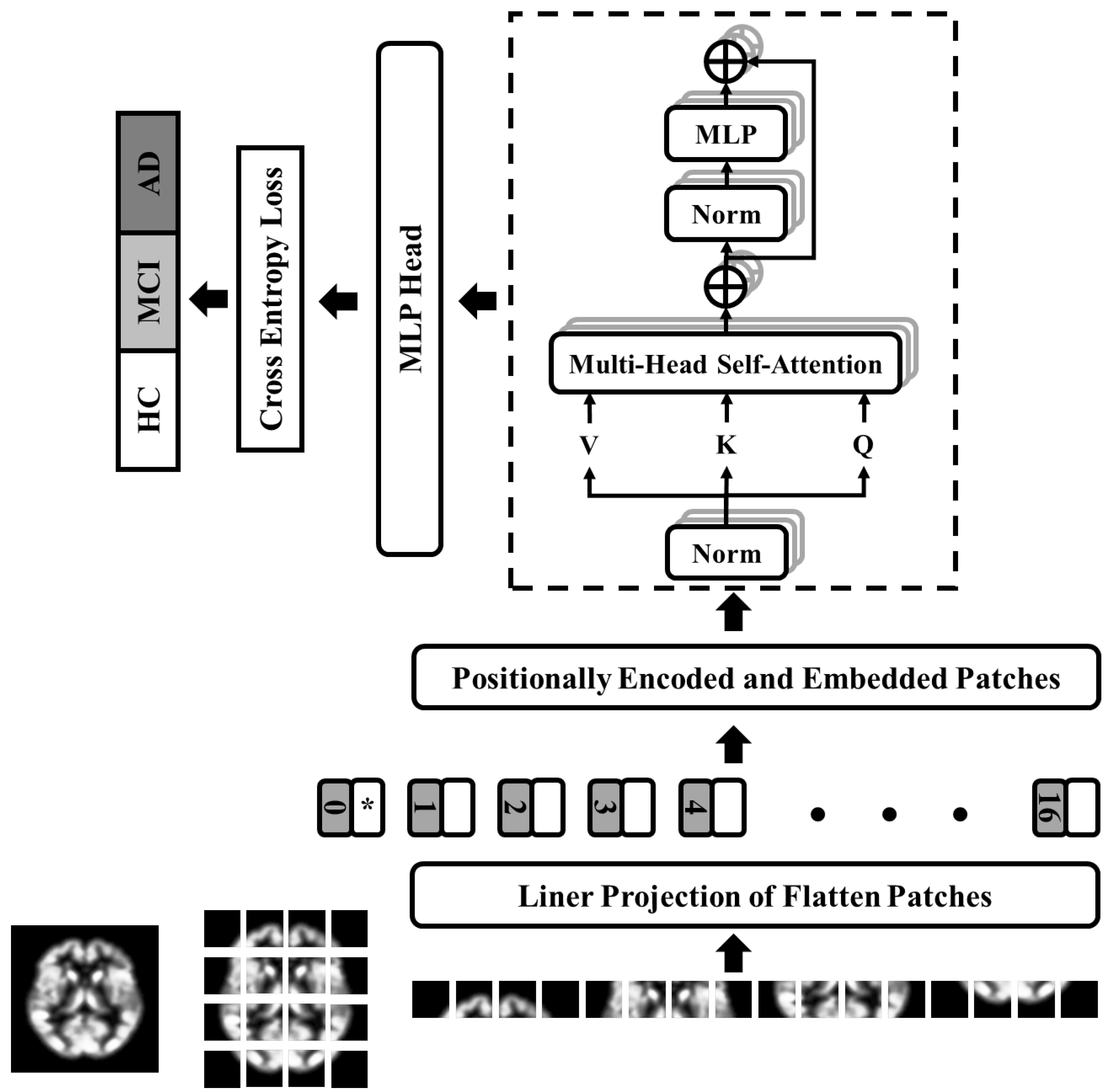
3.4. Proposed Architecture: Optimized Vision Transformer (OViTAD)
3.5. fMRI Pipeline
3.5.1. Data Decomposition from 4D to 2D
3.5.2. Modeling
3.5.3. Subject-Level Evaluation
3.6. Structural Pipeline
3.6.1. Data Split
3.6.2. Data Decomposition 3D to 2D
3.6.3. Modeling
3.6.4. Subject-Level
3.7. Discussion
3.7.1. Technical/Architecture Design
3.7.2. Clinical Observation
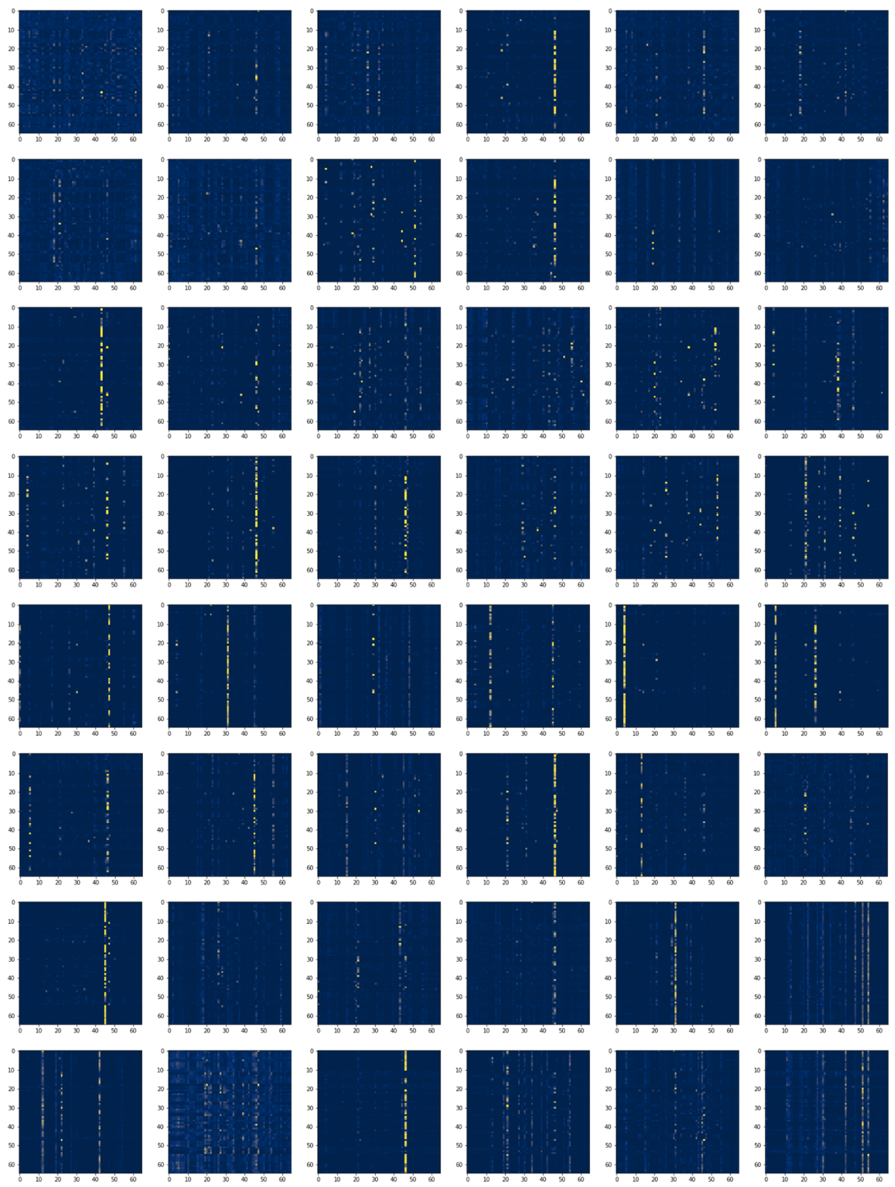
3.7.3. Local and Global Attention Visualization
3.7.4. Limitations
4. Conclusions
Author Contributions
Funding
Institutional Review Board Statement
Informed Consent Statement
Data Availability Statement
Conflicts of Interest
Appendix A

| Model | Dataset | Repetition | Accuracy | Precision macro_avg | Precision weighted_avg | Recall macro_avg | Recall weighted_avg | F1-Score macro_avg | F1-Score weighted_avg | Slices |
|---|---|---|---|---|---|---|---|---|---|---|
| CaIT_AD-HC-MCI | Val | 1 | 0.4984 | 0.4116 | 0.449 | 0.3991 | 0.4984 | 0.3614 | 0.442 | 138600 |
| 2 | 0.4938 | 0.4335 | 0.4598 | 0.3868 | 0.4938 | 0.3519 | 0.4379 | 133560 | ||
| 3 | 0.4877 | 0.4148 | 0.4404 | 0.355 | 0.4877 | 0.2777 | 0.3673 | 134400 | ||
| Test | 1 | 0.5011 | 0.4701 | 0.4865 | 0.402 | 0.5011 | 0.3604 | 0.4396 | 155820 | |
| 2 | 0.4989 | 0.4828 | 0.4895 | 0.4005 | 0.4989 | 0.3577 | 0.4377 | 156100 | ||
| 3 | 0.4691 | 0.3507 | 0.4031 | 0.3723 | 0.4691 | 0.3148 | 0.3865 | 155820 | ||
| CaIT_AD-HCMCI | Val | 1 | 0.8081 | 0.404 | 0.653 | 0.5 | 0.8081 | 0.4469 | 0.7223 | 138600 |
| 2 | 0.8166 | 0.4083 | 0.6668 | 0.5 | 0.8166 | 0.4495 | 0.7341 | 133560 | ||
| 3 | 0.8021 | 0.9011 | 0.8413 | 0.5001 | 0.8021 | 0.4452 | 0.714 | 134400 | ||
| Test | 1 | 0.8113 | 0.4057 | 0.6582 | 0.5 | 0.8113 | 0.4479 | 0.7268 | 155820 | |
| 2 | 0.8117 | 0.4058 | 0.6588 | 0.5 | 0.8117 | 0.448 | 0.7273 | 156100 | ||
| 3 | 0.7979 | 0.8989 | 0.8387 | 0.5 | 0.7979 | 0.4439 | 0.7082 | 155820 | ||
| CaIT_ADMCI-HC | Val | 1 | 0.6799 | 0.6389 | 0.66 | 0.6 | 0.6799 | 0.6007 | 0.6546 | 138600 |
| 2 | 0.675 | 0.6496 | 0.659 | 0.548 | 0.675 | 0.5121 | 0.6002 | 133560 | ||
| 3 | 0.6716 | 0.5506 | 0.5924 | 0.5004 | 0.6716 | 0.4039 | 0.5412 | 134400 | ||
| Test | 1 | 0.6502 | 0.6159 | 0.6291 | 0.568 | 0.6502 | 0.5536 | 0.6071 | 155820 | |
| 2 | 0.6572 | 0.654 | 0.655 | 0.5582 | 0.6572 | 0.5233 | 0.5879 | 156100 | ||
| 3 | 0.6397 | 0.4783 | 0.5239 | 0.4998 | 0.6397 | 0.3923 | 0.5013 | 155820 | ||
| DeepViT_ADMCI_HC | Val | 1 | 0.9723 | 0.9696 | 0.9723 | 0.9681 | 0.9724 | 0.9711 | 0.9723 | 138600 |
| 2 | 0.9904 | 0.9895 | 0.9904 | 0.9903 | 0.9904 | 0.9886 | 0.9904 | 138600 | ||
| 3 | 0.9832 | 0.9812 | 0.9831 | 0.9858 | 0.9834 | 0.9771 | 0.9832 | 133560 | ||
| Test | 1 | 0.9109 | 0.9038 | 0.9105 | 0.9076 | 0.9106 | 0.9004 | 0.9109 | 155820 | |
| 2 | 0.989 | 0.9882 | 0.989 | 0.9894 | 0.989 | 0.9869 | 0.989 | 155820 | ||
| 3 | 0.991 | 0.9904 | 0.991 | 0.9882 | 0.9912 | 0.9928 | 0.991 | 156100 | ||
| DeepViT_AD_HCMCI | Val | 1 | 0.9618 | 0.935 | 0.9607 | 0.9618 | 0.9618 | 0.9131 | 0.9618 | 138600 |
| 2 | 0.9831 | 0.9719 | 0.9831 | 0.9695 | 0.9832 | 0.9743 | 0.9831 | 133560 | ||
| 3 | 0.9875 | 0.9804 | 0.9875 | 0.9779 | 0.9876 | 0.983 | 0.9875 | 134400 | ||
| Test | 1 | 0.9807 | 0.9683 | 0.9806 | 0.9698 | 0.9806 | 0.9668 | 0.9807 | 155820 | |
| 2 | 0.9719 | 0.954 | 0.9719 | 0.9542 | 0.9719 | 0.9538 | 0.9719 | 156100 | ||
| 3 | 0.9315 | 0.8818 | 0.9275 | 0.9381 | 0.9325 | 0.8451 | 0.9315 | 155820 | ||
| DeepViT_AD_HC_MCI | Val | 1 | 0.9387 | 0.9322 | 0.9385 | 0.9358 | 0.9392 | 0.9296 | 0.9387 | 138600 |
| 2 | 0.935 | 0.9352 | 0.9352 | 0.9365 | 0.9361 | 0.9347 | 0.935 | 133560 | ||
| 3 | 0.9299 | 0.9323 | 0.9299 | 0.9282 | 0.9303 | 0.937 | 0.9299 | 134400 | ||
| Test | 1 | 0.8997 | 0.9049 | 0.8995 | 0.9019 | 0.8996 | 0.9083 | 0.8997 | 155820 | |
| 2 | 0.9069 | 0.9092 | 0.9069 | 0.9123 | 0.9078 | 0.9069 | 0.9069 | 156100 | ||
| 3 | 0.8855 | 0.8727 | 0.8837 | 0.8954 | 0.8879 | 0.8589 | 0.8855 | 155820 | ||
| ViT24_8_ADMCI_HC | Val | 1 | 0.9772 | 0.975 | 0.9773 | 0.9723 | 0.9775 | 0.978 | 0.9772 | 138600 |
| 2 | 0.9572 | 0.9527 | 0.9572 | 0.9514 | 0.9573 | 0.954 | 0.9572 | 133560 | ||
| 3 | 0.9507 | 0.9442 | 0.9507 | 0.943 | 0.9508 | 0.9455 | 0.9507 | 134400 | ||
| Test | 1 | 0.9181 | 0.9112 | 0.9176 | 0.9166 | 0.9179 | 0.9068 | 0.9181 | 155820 | |
| 2 | 0.9396 | 0.9348 | 0.9393 | 0.9387 | 0.9395 | 0.9314 | 0.9396 | 156100 | ||
| 3 | 0.9461 | 0.9412 | 0.946 | 0.9438 | 0.946 | 0.9388 | 0.9461 | 155820 | ||
| ViT24_8_AD_HCMCI | Val | 1 | 0.9738 | 0.9564 | 0.9734 | 0.9708 | 0.9736 | 0.9436 | 0.9738 | 138600 |
| 2 | 0.9849 | 0.9747 | 0.9849 | 0.9761 | 0.9848 | 0.9733 | 0.9849 | 133560 | ||
| 3 | 0.9894 | 0.9834 | 0.9894 | 0.9784 | 0.9896 | 0.9886 | 0.9894 | 134400 | ||
| Test | 1 | 0.9782 | 0.965 | 0.9784 | 0.9571 | 0.9788 | 0.9734 | 0.9782 | 155820 | |
| 2 | 0.9856 | 0.9765 | 0.9856 | 0.9743 | 0.9856 | 0.9787 | 0.9856 | 156100 | ||
| 3 | 0.932 | 0.8852 | 0.9289 | 0.9274 | 0.9314 | 0.8552 | 0.932 | 155820 | ||
| ViT24_8_AD_HC_MCI | Val | 1 | 0.9491 | 0.943 | 0.9487 | 0.9485 | 0.9497 | 0.9392 | 0.9491 | 138600 |
| 2 | 0.9318 | 0.9328 | 0.932 | 0.9313 | 0.9334 | 0.9354 | 0.9318 | 133560 | ||
| 3 | 0.922 | 0.9241 | 0.9218 | 0.9183 | 0.9223 | 0.9308 | 0.922 | 134400 | ||
| Test | 1 | 0.9137 | 0.9174 | 0.9135 | 0.9149 | 0.9137 | 0.9202 | 0.9137 | 155820 | |
| 2 | 0.9207 | 0.9232 | 0.9207 | 0.9226 | 0.9208 | 0.9241 | 0.9207 | 156100 | ||
| 3 | 0.887 | 0.8705 | 0.885 | 0.8871 | 0.8871 | 0.8596 | 0.887 | 155820 | ||
| ViT_vanilla_ADMCI_HC | Val | 1 | 0.9653 | 0.9622 | 0.9655 | 0.9581 | 0.9661 | 0.9669 | 0.9653 | 138600 |
| 2 | 0.9376 | 0.9308 | 0.9376 | 0.9312 | 0.9376 | 0.9304 | 0.9376 | 133560 | ||
| 3 | 0.9445 | 0.9368 | 0.9444 | 0.9381 | 0.9443 | 0.9357 | 0.9445 | 134400 | ||
| Test | 1 | 0.9352 | 0.9298 | 0.9348 | 0.9351 | 0.9352 | 0.9253 | 0.9352 | 155820 | |
| 2 | 0.9198 | 0.9117 | 0.9185 | 0.9278 | 0.922 | 0.9011 | 0.9198 | 156100 | ||
| 3 | 0.9406 | 0.9355 | 0.9406 | 0.9355 | 0.9406 | 0.9355 | 0.9406 | 155820 | ||
| ViT_vanilla_AD_HCMCI | Val | 1 | 0.9663 | 0.9431 | 0.9655 | 0.9656 | 0.9662 | 0.924 | 0.9663 | 138600 |
| 2 | 0.9777 | 0.9634 | 0.9779 | 0.9568 | 0.9782 | 0.9702 | 0.9777 | 133560 | ||
| 3 | 0.9866 | 0.9791 | 0.9867 | 0.9748 | 0.9868 | 0.9836 | 0.9866 | 134400 | ||
| Test | 1 | 0.9837 | 0.9735 | 0.9837 | 0.9696 | 0.9839 | 0.9776 | 0.9837 | 155820 | |
| 2 | 0.9706 | 0.9515 | 0.9705 | 0.9559 | 0.9704 | 0.9472 | 0.9706 | 156100 | ||
| 3 | 0.9213 | 0.8677 | 0.9179 | 0.906 | 0.9195 | 0.8402 | 0.9213 | 155820 | ||
| ViT_vanilla_AD_HC_MCI | Val | 1 | 0.9359 | 0.9245 | 0.935 | 0.9329 | 0.9355 | 0.9183 | 0.9359 | 138600 |
| 2 | 0.9095 | 0.9092 | 0.9095 | 0.9027 | 0.9112 | 0.9174 | 0.9095 | 133560 | ||
| 3 | 0.9255 | 0.9285 | 0.9255 | 0.927 | 0.9256 | 0.93 | 0.9255 | 134400 | ||
| Test | 1 | 0.9158 | 0.9194 | 0.9155 | 0.9248 | 0.9182 | 0.9165 | 0.9158 | 155820 | |
| 2 | 0.9074 | 0.9071 | 0.9072 | 0.9073 | 0.9088 | 0.9085 | 0.9074 | 156100 | ||
| 3 | 0.8876 | 0.8653 | 0.8839 | 0.8947 | 0.8901 | 0.85 | 0.8876 | 155820 | ||
| OViTAD_ADMCI_HC | Val | 1 | 0.9636 | 0.9602 | 0.9637 | 0.9576 | 0.964 | 0.9629 | 0.9636 | 138600 |
| 2 | 0.9501 | 0.9445 | 0.95 | 0.9459 | 0.9499 | 0.9431 | 0.9501 | 133560 | ||
| 3 | 0.9435 | 0.9362 | 0.9436 | 0.9345 | 0.9438 | 0.938 | 0.9435 | 134400 | ||
| Test | 1 | 0.9146 | 0.9073 | 0.914 | 0.9134 | 0.9144 | 0.9024 | 0.9146 | 155820 | |
| 2 | 0.9281 | 0.9211 | 0.9271 | 0.9348 | 0.9297 | 0.9116 | 0.9281 | 156100 | ||
| 3 | 0.9221 | 0.9155 | 0.9222 | 0.9152 | 0.9222 | 0.9159 | 0.9221 | 155820 | ||
| OViTAD_AD_HCMCI | Val | 1 | 0.9539 | 0.9218 | 0.9527 | 0.9467 | 0.9534 | 0.9012 | 0.9539 | 138600 |
| 2 | 0.9754 | 0.9586 | 0.9753 | 0.9621 | 0.9753 | 0.9553 | 0.9754 | 133560 | ||
| 3 | 0.9854 | 0.9773 | 0.9855 | 0.9727 | 0.9856 | 0.9819 | 0.9854 | 134400 | ||
| Test | 1 | 0.9699 | 0.9511 | 0.97 | 0.9482 | 0.9701 | 0.9541 | 0.9699 | 155820 | |
| 2 | 0.9843 | 0.9749 | 0.9845 | 0.9653 | 0.985 | 0.9853 | 0.9843 | 156100 | ||
| 3 | 0.9205 | 0.867 | 0.9173 | 0.9022 | 0.9184 | 0.8412 | 0.9205 | 155820 | ||
| OViTAD_AD_HC_MCI | Val | 1 | 0.9239 | 0.914 | 0.9232 | 0.925 | 0.924 | 0.9055 | 0.9239 | 138600 |
| 2 | 0.9102 | 0.91 | 0.9102 | 0.9097 | 0.9112 | 0.9111 | 0.9102 | 133560 | ||
| 3 | 0.9192 | 0.9219 | 0.9193 | 0.917 | 0.921 | 0.9283 | 0.9192 | 134400 | ||
| Test | 1 | 0.8939 | 0.9026 | 0.8936 | 0.9057 | 0.8949 | 0.9009 | 0.8939 | 155820 | |
| 2 | 0.9025 | 0.9053 | 0.9024 | 0.9038 | 0.9024 | 0.907 | 0.9025 | 156100 | ||
| 3 | 0.8882 | 0.8682 | 0.8852 | 0.891 | 0.889 | 0.8557 | 0.8882 | 155820 | ||
| OViTAD_AD_HC | Val | 1 | 0.9615 | 0.9639 | 0.9618 | 0.9519 | 0.9615 | 0.9574 | 0.9612 | 74900 |
| 2 | 0.9877 | 0.989 | 0.9878 | 0.984 | 0.9877 | 0.9864 | 0.9877 | 70420 | ||
| 3 | 0.9815 | 0.9775 | 0.982 | 0.9838 | 0.9815 | 0.9804 | 0.9816 | 70700 | ||
| Test | 1 | 0.9608 | 0.9501 | 0.9627 | 0.9653 | 0.9608 | 0.9569 | 0.9611 | 87220 | |
| 2 | 0.9545 | 0.9429 | 0.9568 | 0.9589 | 0.9545 | 0.95 | 0.9549 | 87500 | ||
| 3 | 0.8946 | 0.9004 | 0.8962 | 0.8694 | 0.8946 | 0.8814 | 0.8925 | 87500 | ||
| OViTAD_HC_MCI | Val | 1 | 0.9596 | 0.9576 | 0.9602 | 0.9608 | 0.9596 | 0.959 | 0.9597 | 112000 |
| 2 | 0.9265 | 0.9231 | 0.9277 | 0.928 | 0.9265 | 0.9251 | 0.9267 | 109060 | ||
| 3 | 0.9283 | 0.9243 | 0.929 | 0.9285 | 0.9283 | 0.9262 | 0.9285 | 107800 | ||
| Test | 1 | 0.9038 | 0.9049 | 0.9041 | 0.9013 | 0.9038 | 0.9027 | 0.9036 | 126420 | |
| 2 | 0.8921 | 0.8934 | 0.8926 | 0.8894 | 0.8921 | 0.8909 | 0.8918 | 126700 | ||
| 3 | 0.9419 | 0.9429 | 0.9421 | 0.9398 | 0.9419 | 0.9411 | 0.9418 | 124320 |
| Model | Dataset | Repetition | Accuracy | Precision macro_avg | Precision weighted_avg | Recall macro_avg | Recall weighted_avg | F1-Score macro_avg | F1-Score weighted_avg | Subjects |
|---|---|---|---|---|---|---|---|---|---|---|
| CaIT_AD-HC-MCI | Val | 1 | 0.5926 | 0.4127 | 0.4974 | 0.4558 | 0.5926 | 0.4131 | 0.5176 | 27 |
| 2 | 0.5556 | 0.3818 | 0.4626 | 0.4188 | 0.5556 | 0.3714 | 0.473 | 27 | ||
| 3 | 0.4815 | 0.1605 | 0.2318 | 0.3333 | 0.4815 | 0.2167 | 0.313 | 27 | ||
| Test | 1 | 0.4516 | 0.3148 | 0.3781 | 0.3463 | 0.4516 | 0.284 | 0.359 | 31 | |
| 2 | 0.4839 | 0.3 | 0.3677 | 0.3701 | 0.4839 | 0.3 | 0.3823 | 31 | ||
| 3 | 0.4516 | 0.3148 | 0.3781 | 0.3463 | 0.4516 | 0.284 | 0.359 | 31 | ||
| CaIT_AD-HCMCI | Val | 1 | 0.8148 | 0.4074 | 0.6639 | 0.5 | 0.8148 | 0.449 | 0.7317 | 27 |
| 2 | 0.8148 | 0.4074 | 0.6639 | 0.5 | 0.8148 | 0.449 | 0.7317 | 27 | ||
| 3 | 0.8148 | 0.4074 | 0.6639 | 0.5 | 0.8148 | 0.449 | 0.7317 | 27 | ||
| Test | 1 | 0.8065 | 0.4032 | 0.6504 | 0.5 | 0.8065 | 0.4464 | 0.72 | 31 | |
| 2 | 0.8065 | 0.4032 | 0.6504 | 0.5 | 0.8065 | 0.4464 | 0.72 | 31 | ||
| 3 | 0.8065 | 0.4032 | 0.6504 | 0.5 | 0.8065 | 0.4464 | 0.72 | 31 | ||
| CaIT_ADMCI-HC | Val | 1 | 0.7037 | 0.6875 | 0.6944 | 0.5833 | 0.7037 | 0.5714 | 0.6508 | 27 |
| 2 | 0.6667 | 0.3333 | 0.4444 | 0.5 | 0.6667 | 0.4 | 0.5333 | 27 | ||
| 3 | 0.6667 | 0.3333 | 0.4444 | 0.5 | 0.6667 | 0.4 | 0.5333 | 27 | ||
| Test | 1 | 0.6452 | 0.3226 | 0.4162 | 0.5 | 0.6452 | 0.3922 | 0.506 | 31 | |
| 2 | 0.6774 | 0.8333 | 0.7849 | 0.5455 | 0.6774 | 0.4833 | 0.5753 | 31 | ||
| 3 | 0.6452 | 0.3226 | 0.4162 | 0.5 | 0.6452 | 0.3922 | 0.506 | 31 | ||
| DeepViT_ADMCI_HC | Val | 1 | 1 | 1 | 1 | 1 | 1 | 1 | 1 | 27 |
| 2 | 1 | 1 | 1 | 1 | 1 | 1 | 1 | 27 | ||
| 3 | 1 | 1 | 1 | 1 | 1 | 1 | 1 | 27 | ||
| Test | 1 | 0.9677 | 0.964 | 0.9674 | 0.9762 | 0.9693 | 0.9545 | 0.9677 | 31 | |
| 2 | 1 | 1 | 1 | 1 | 1 | 1 | 1 | 31 | ||
| 3 | 1 | 1 | 1 | 1 | 1 | 1 | 1 | 31 | ||
| DeepViT_AD_HCMCI | Val | 1 | 0.963 | 0.9333 | 0.9613 | 0.9783 | 0.9646 | 0.9 | 0.963 | 27 |
| 2 | 1 | 1 | 1 | 1 | 1 | 1 | 1 | 27 | ||
| 3 | 1 | 1 | 1 | 1 | 1 | 1 | 1 | 27 | ||
| Test | 1 | 1 | 1 | 1 | 1 | 1 | 1 | 1 | 31 | |
| 2 | 1 | 1 | 1 | 1 | 1 | 1 | 1 | 31 | ||
| 3 | 0.9677 | 0.9447 | 0.9666 | 0.9808 | 0.969 | 0.9167 | 0.9677 | 31 | ||
| DeepViT_AD_HC_MCI | Val | 1 | 1 | 1 | 1 | 1 | 1 | 1 | 1 | 27 |
| 2 | 1 | 1 | 1 | 1 | 1 | 1 | 1 | 27 | ||
| 3 | 1 | 1 | 1 | 1 | 1 | 1 | 1 | 27 | ||
| Test | 1 | 0.9677 | 0.9726 | 0.9675 | 0.9778 | 0.9699 | 0.9697 | 0.9677 | 31 | |
| 2 | 0.9677 | 0.9726 | 0.9675 | 0.9778 | 0.9699 | 0.9697 | 0.9677 | 31 | ||
| 3 | 0.9355 | 0.9316 | 0.9354 | 0.9583 | 0.9435 | 0.9141 | 0.9355 | 31 | ||
| ViT24_8_ADMCI_HC | Val | 1 | 1 | 1 | 1 | 1 | 1 | 1 | 1 | 27 |
| 2 | 1 | 1 | 1 | 1 | 1 | 1 | 1 | 27 | ||
| 3 | 1 | 1 | 1 | 1 | 1 | 1 | 1 | 27 | ||
| Test | 1 | 0.9677 | 0.964 | 0.9674 | 0.9762 | 0.9693 | 0.9545 | 0.9677 | 31 | |
| 2 | 0.9677 | 0.964 | 0.9674 | 0.9762 | 0.9693 | 0.9545 | 0.9677 | 31 | ||
| 3 | 0.9677 | 0.964 | 0.9674 | 0.9762 | 0.9693 | 0.9545 | 0.9677 | 31 | ||
| ViT24_8_AD_HCMCI | Val | 1 | 1 | 1 | 1 | 1 | 1 | 1 | 1 | 27 |
| 2 | 1 | 1 | 1 | 1 | 1 | 1 | 1 | 27 | ||
| 3 | 1 | 1 | 1 | 1 | 1 | 1 | 1 | 27 | ||
| Test | 1 | 1 | 1 | 1 | 1 | 1 | 1 | 1 | 31 | |
| 2 | 1 | 1 | 1 | 1 | 1 | 1 | 1 | 31 | ||
| 3 | 0.9677 | 0.9447 | 0.9666 | 0.9808 | 0.969 | 0.9167 | 0.9677 | 31 | ||
| ViT24_8_AD_HC_MCI | Val | 1 | 1 | 1 | 1 | 1 | 1 | 1 | 1 | 27 |
| 2 | 1 | 1 | 1 | 1 | 1 | 1 | 1 | 27 | ||
| 3 | 0.963 | 0.968 | 0.9626 | 0.9762 | 0.9656 | 0.963 | 0.963 | 27 | ||
| Test | 1 | 1 | 1 | 1 | 1 | 1 | 1 | 1 | 31 | |
| 2 | 0.9677 | 0.9726 | 0.9675 | 0.9778 | 0.9699 | 0.9697 | 0.9677 | 31 | ||
| 3 | 0.9355 | 0.9316 | 0.9354 | 0.9583 | 0.9435 | 0.9141 | 0.9355 | 31 | ||
| ViT_vanilla_ADMCI_HC | Val | 1 | 1 | 1 | 1 | 1 | 1 | 1 | 1 | 27 |
| 2 | 1 | 1 | 1 | 1 | 1 | 1 | 1 | 27 | ||
| 3 | 1 | 1 | 1 | 1 | 1 | 1 | 1 | 27 | ||
| Test | 1 | 0.9677 | 0.964 | 0.9674 | 0.9762 | 0.9693 | 0.9545 | 0.9677 | 31 | |
| 2 | 0.9677 | 0.964 | 0.9674 | 0.9762 | 0.9693 | 0.9545 | 0.9677 | 31 | ||
| 3 | 1 | 1 | 1 | 1 | 1 | 1 | 1 | 31 | ||
| ViT_vanilla_AD_HCMCI | Val | 1 | 1 | 1 | 1 | 1 | 1 | 1 | 1 | 27 |
| 2 | 1 | 1 | 1 | 1 | 1 | 1 | 1 | 27 | ||
| 3 | 1 | 1 | 1 | 1 | 1 | 1 | 1 | 27 | ||
| Test | 1 | 1 | 1 | 1 | 1 | 1 | 1 | 1 | 31 | |
| 2 | 1 | 1 | 1 | 1 | 1 | 1 | 1 | 31 | ||
| 3 | 0.9677 | 0.9447 | 0.9666 | 0.9808 | 0.969 | 0.9167 | 0.9677 | 31 | ||
| ViT_vanilla_AD_HC_MCI | Val | 1 | 1 | 1 | 1 | 1 | 1 | 1 | 1 | 27 |
| 2 | 1 | 1 | 1 | 1 | 1 | 1 | 1 | 27 | ||
| 3 | 0.963 | 0.9691 | 0.9632 | 0.9667 | 0.9667 | 0.9744 | 0.963 | 27 | ||
| Test | 1 | 0.9677 | 0.9726 | 0.9675 | 0.9778 | 0.9699 | 0.9697 | 0.9677 | 31 | |
| 2 | 0.9677 | 0.9726 | 0.9675 | 0.9778 | 0.9699 | 0.9697 | 0.9677 | 31 | ||
| 3 | 0.9677 | 0.9582 | 0.9668 | 0.9778 | 0.9699 | 0.9444 | 0.9677 | 31 | ||
| OViTAD_ADMCI_HC | Val | 1 | 1 | 1 | 1 | 1 | 1 | 1 | 1 | 27 |
| 2 | 1 | 1 | 1 | 1 | 1 | 1 | 1 | 27 | ||
| 3 | 1 | 1 | 1 | 1 | 1 | 1 | 1 | 27 | ||
| Test | 1 | 0.9677 | 0.964 | 0.9674 | 0.9762 | 0.9693 | 0.9545 | 0.9677 | 31 | |
| 2 | 0.9677 | 0.964 | 0.9674 | 0.9762 | 0.9693 | 0.9545 | 0.9677 | 31 | ||
| 3 | 1 | 1 | 1 | 1 | 1 | 1 | 1 | 31 | ||
| OViTAD_AD_HCMCI | Val | 1 | 0.963 | 0.9333 | 0.9613 | 0.9783 | 0.9646 | 0.9 | 0.963 | 27 |
| 2 | 1 | 1 | 1 | 1 | 1 | 1 | 1 | 27 | ||
| 3 | 1 | 1 | 1 | 1 | 1 | 1 | 1 | 27 | ||
| Test | 1 | 1 | 1 | 1 | 1 | 1 | 1 | 1 | 31 | |
| 2 | 1 | 1 | 1 | 1 | 1 | 1 | 1 | 31 | ||
| 3 | 0.9677 | 0.9447 | 0.9666 | 0.9808 | 0.969 | 0.9167 | 0.9677 | 31 | ||
| OViTAD_AD_HC_MCI | Val | 1 | 1 | 1 | 1 | 1 | 1 | 1 | 1 | 27 |
| 2 | 0.963 | 0.9691 | 0.9632 | 0.9667 | 0.9667 | 0.9744 | 0.963 | 27 | ||
| 3 | 1 | 1 | 1 | 1 | 1 | 1 | 1 | 27 | ||
| Test | 1 | 0.9677 | 0.9726 | 0.9675 | 0.9778 | 0.9699 | 0.9697 | 0.9677 | 31 | |
| 2 | 0.9677 | 0.9726 | 0.9675 | 0.9778 | 0.9699 | 0.9697 | 0.9677 | 31 | ||
| 3 | 0.9677 | 0.9582 | 0.9668 | 0.9778 | 0.9699 | 0.9444 | 0.9677 | 31 | ||
| OViTAD_AD_HC | Val | 1 | 1 | 1 | 1 | 1 | 1 | 1 | 1 | 14 |
| 2 | 1 | 1 | 1 | 1 | 1 | 1 | 1 | 14 | ||
| 3 | 1 | 1 | 1 | 1 | 1 | 1 | 1 | 14 | ||
| Test | 1 | 1 | 1 | 1 | 1 | 1 | 1 | 1 | 17 | |
| 2 | 1 | 1 | 1 | 1 | 1 | 1 | 1 | 17 | ||
| 3 | 0.9412 | 0.9583 | 0.9461 | 0.9167 | 0.9412 | 0.9328 | 0.9398 | 17 | ||
| OViTAD_HC_MCI | Val | 1 | 1 | 1 | 1 | 1 | 1 | 1 | 1 | 22 |
| 2 | 1 | 1 | 1 | 1 | 1 | 1 | 1 | 22 | ||
| 3 | 1 | 1 | 1 | 1 | 1 | 1 | 1 | 22 | ||
| Test | 1 | 0.96 | 0.9667 | 0.9627 | 0.9545 | 0.96 | 0.9589 | 0.9597 | 25 | |
| 2 | 0.96 | 0.9667 | 0.9627 | 0.9545 | 0.96 | 0.9589 | 0.9597 | 25 | ||
| 3 | 1 | 1 | 1 | 1 | 1 | 1 | 1 | 25 |
| Model | Dataset | Repetition | Accuracy | Precision macro_avg | Precision weighted_avg | Recall macro_avg | Recall weighted_avg | F1-Score macro_avg | F1-Score weighted_avg | Slices |
|---|---|---|---|---|---|---|---|---|---|---|
| CaIT_ADMCI-HC_S3 | Val | 1 | 0.9317 | 0.7997 | 0.9143 | 0.5188 | 0.9317 | 0.5191 | 0.9025 | 11040 |
| 2 | 0.9316 | 0.7603 | 0.9098 | 0.5272 | 0.9316 | 0.5345 | 0.9046 | 11027 | ||
| 3 | 0.931 | 0.7762 | 0.9105 | 0.5191 | 0.931 | 0.5197 | 0.9018 | 11040 | ||
| Test | 1 | 0.921 | 0.797 | 0.9021 | 0.5243 | 0.921 | 0.5265 | 0.8886 | 11413 | |
| 2 | 0.9198 | 0.7524 | 0.8941 | 0.5177 | 0.9198 | 0.5145 | 0.8861 | 11427 | ||
| 3 | 0.9213 | 0.797 | 0.9025 | 0.5253 | 0.9213 | 0.5284 | 0.8892 | 11455 | ||
| CaIT_AD-HCMCI_S3 | Val | 1 | 0.6912 | 0.6796 | 0.6854 | 0.657 | 0.6912 | 0.6602 | 0.681 | 11040 |
| 2 | 0.6753 | 0.6604 | 0.668 | 0.6412 | 0.6753 | 0.6436 | 0.6651 | 11027 | ||
| 3 | 0.6645 | 0.6482 | 0.6559 | 0.6262 | 0.6645 | 0.6274 | 0.6513 | 11040 | ||
| Test | 1 | 0.6687 | 0.6526 | 0.6609 | 0.6349 | 0.6687 | 0.637 | 0.6586 | 11413 | |
| 2 | 0.6619 | 0.6443 | 0.6532 | 0.6264 | 0.6619 | 0.6279 | 0.6507 | 11427 | ||
| 3 | 0.672 | 0.6563 | 0.6644 | 0.6378 | 0.672 | 0.64 | 0.6618 | 11455 | ||
| CaIT_AD-HC-MCI_S3 | Val | 1 | 0.6757 | 0.6941 | 0.6764 | 0.4826 | 0.6757 | 0.479 | 0.6498 | 11040 |
| 2 | 0.6637 | 0.6583 | 0.6595 | 0.4656 | 0.6637 | 0.4533 | 0.6354 | 11027 | ||
| 3 | 0.6591 | 0.616 | 0.6478 | 0.4832 | 0.6591 | 0.4919 | 0.6337 | 11040 | ||
| Test | 1 | 0.6496 | 0.6409 | 0.6442 | 0.4701 | 0.6496 | 0.464 | 0.6208 | 11413 | |
| 2 | 0.6331 | 0.6646 | 0.637 | 0.448 | 0.6331 | 0.4311 | 0.6004 | 11427 | ||
| 3 | 0.6675 | 0.6157 | 0.6538 | 0.4972 | 0.6675 | 0.5038 | 0.6419 | 11455 | ||
| DeepViT_ADMCI_HC_S3 | Val | 1 | 0.9898 | 0.958 | 0.9894 | 0.9883 | 0.9897 | 0.9318 | 0.9898 | 11027 |
| 2 | 0.9901 | 0.9604 | 0.9899 | 0.9796 | 0.99 | 0.943 | 0.9901 | 11040 | ||
| 3 | 0.9829 | 0.9326 | 0.9827 | 0.9444 | 0.9825 | 0.9215 | 0.9829 | 11040 | ||
| Test | 1 | 0.9891 | 0.9618 | 0.9889 | 0.9859 | 0.9891 | 0.9405 | 0.9891 | 11427 | |
| 2 | 0.9892 | 0.9618 | 0.9889 | 0.9897 | 0.9892 | 0.9375 | 0.9892 | 11413 | ||
| 3 | 0.9869 | 0.9546 | 0.9867 | 0.9691 | 0.9867 | 0.9412 | 0.9869 | 11455 | ||
| DeepViT_AD_HCMCI_S3 | Val | 1 | 0.9452 | 0.9421 | 0.9448 | 0.9494 | 0.9462 | 0.9367 | 0.9452 | 11027 |
| 2 | 0.9505 | 0.948 | 0.9503 | 0.9519 | 0.9507 | 0.9448 | 0.9505 | 11040 | ||
| 3 | 0.9186 | 0.9137 | 0.9178 | 0.9225 | 0.9196 | 0.9076 | 0.9186 | 11040 | ||
| Test | 1 | 0.9404 | 0.9369 | 0.9399 | 0.9454 | 0.9416 | 0.9308 | 0.9404 | 11427 | |
| 2 | 0.9458 | 0.943 | 0.9455 | 0.9473 | 0.946 | 0.9394 | 0.9458 | 11413 | ||
| 3 | 0.9245 | 0.9195 | 0.9236 | 0.9323 | 0.927 | 0.9114 | 0.9245 | 11455 | ||
| DeepViT_AD_HC_MCI_S3 | Val | 1 | 0.9255 | 0.9152 | 0.9248 | 0.9398 | 0.9284 | 0.8959 | 0.9255 | 11040 |
| 2 | 0.9176 | 0.9028 | 0.917 | 0.9235 | 0.9183 | 0.8855 | 0.9176 | 11027 | ||
| 3 | 0.9149 | 0.9058 | 0.9147 | 0.9292 | 0.9155 | 0.8865 | 0.9149 | 11040 | ||
| Test | 1 | 0.9202 | 0.9079 | 0.9193 | 0.9388 | 0.9241 | 0.8849 | 0.9202 | 11413 | |
| 2 | 0.9103 | 0.9014 | 0.9099 | 0.9096 | 0.911 | 0.8945 | 0.9103 | 11427 | ||
| 3 | 0.9208 | 0.9156 | 0.9206 | 0.9364 | 0.9215 | 0.8982 | 0.9208 | 11455 | ||
| ViT44_8_ADMCI_HC_S3 | Val | 1 | 0.9912 | 0.965 | 0.9911 | 0.9797 | 0.9911 | 0.9512 | 0.9912 | 11027 |
| 2 | 0.9913 | 0.9653 | 0.9912 | 0.9817 | 0.9912 | 0.9502 | 0.9913 | 11040 | ||
| 3 | 0.9851 | 0.9402 | 0.9847 | 0.9603 | 0.9847 | 0.9221 | 0.9851 | 11040 | ||
| Test | 1 | 0.9911 | 0.9693 | 0.991 | 0.9821 | 0.991 | 0.9573 | 0.9911 | 11427 | |
| 2 | 0.9892 | 0.9624 | 0.989 | 0.9827 | 0.9891 | 0.9439 | 0.9892 | 11413 | ||
| 3 | 0.9846 | 0.9465 | 0.9844 | 0.9637 | 0.9843 | 0.9306 | 0.9846 | 11455 | ||
| ViT44_8_AD_HCMCI_S3 | Val | 1 | 0.9607 | 0.9587 | 0.9606 | 0.963 | 0.9611 | 0.9552 | 0.9607 | 11027 |
| 2 | 0.9636 | 0.9617 | 0.9634 | 0.967 | 0.9642 | 0.9574 | 0.9636 | 11040 | ||
| 3 | 0.9372 | 0.9341 | 0.937 | 0.9376 | 0.9373 | 0.9311 | 0.9372 | 11040 | ||
| Test | 1 | 0.9616 | 0.9595 | 0.9614 | 0.9653 | 0.9623 | 0.9549 | 0.9616 | 11427 | |
| 2 | 0.962 | 0.9599 | 0.9618 | 0.9658 | 0.9627 | 0.9553 | 0.962 | 11413 | ||
| 3 | 0.9362 | 0.9327 | 0.9358 | 0.9383 | 0.9366 | 0.9284 | 0.9362 | 11455 | ||
| ViT44_8_AD_HC_MCI_S3 | Val | 1 | 0.9359 | 0.93 | 0.9358 | 0.9425 | 0.9361 | 0.9189 | 0.9359 | 11040 |
| 2 | 0.9279 | 0.9158 | 0.9277 | 0.9232 | 0.9279 | 0.9088 | 0.9279 | 11027 | ||
| 3 | 0.9287 | 0.9209 | 0.9283 | 0.928 | 0.93 | 0.9155 | 0.9287 | 11040 | ||
| Test | 1 | 0.9339 | 0.9243 | 0.9337 | 0.9407 | 0.9342 | 0.9101 | 0.9339 | 11413 | |
| 2 | 0.9228 | 0.9179 | 0.9227 | 0.9175 | 0.9228 | 0.9185 | 0.9228 | 11427 | ||
| 3 | 0.9277 | 0.9219 | 0.9272 | 0.9291 | 0.9295 | 0.917 | 0.9277 | 11455 | ||
| ViT_vanilla_ADMCI_HC_S3 | Val | 1 | 0.9916 | 0.9658 | 0.9914 | 0.9901 | 0.9915 | 0.9442 | 0.9916 | 11027 |
| 2 | 0.9915 | 0.9665 | 0.9914 | 0.9765 | 0.9914 | 0.9569 | 0.9915 | 11040 | ||
| 3 | 0.986 | 0.9433 | 0.9856 | 0.9688 | 0.9857 | 0.9208 | 0.986 | 11040 | ||
| Test | 1 | 0.9898 | 0.9643 | 0.9896 | 0.989 | 0.9898 | 0.9424 | 0.9898 | 11427 | |
| 2 | 0.9892 | 0.9621 | 0.989 | 0.9864 | 0.9892 | 0.9405 | 0.9892 | 11413 | ||
| 3 | 0.9844 | 0.9455 | 0.9841 | 0.9635 | 0.9841 | 0.929 | 0.9844 | 11455 | ||
| ViT_vanilla_AD_HCMCI_S3 | Val | 1 | 0.9598 | 0.9577 | 0.9596 | 0.9632 | 0.9604 | 0.9533 | 0.9598 | 11027 |
| 2 | 0.9566 | 0.9541 | 0.9563 | 0.9619 | 0.9578 | 0.9484 | 0.9566 | 11040 | ||
| 3 | 0.9262 | 0.9225 | 0.9259 | 0.9257 | 0.9261 | 0.9198 | 0.9262 | 11040 | ||
| Test | 1 | 0.9585 | 0.9562 | 0.9582 | 0.9634 | 0.9596 | 0.9507 | 0.9585 | 11427 | |
| 2 | 0.9545 | 0.952 | 0.9542 | 0.9596 | 0.9557 | 0.9463 | 0.9545 | 11413 | ||
| 3 | 0.9319 | 0.928 | 0.9314 | 0.9354 | 0.9327 | 0.9226 | 0.9319 | 11455 | ||
| ViT_vanilla_AD_HC_MCI_S3 | Val | 1 | 0.9439 | 0.9408 | 0.9437 | 0.9497 | 0.9443 | 0.9329 | 0.9439 | 11040 |
| 2 | 0.924 | 0.9109 | 0.9237 | 0.9274 | 0.9241 | 0.8966 | 0.924 | 11027 | ||
| 3 | 0.9267 | 0.911 | 0.9264 | 0.9204 | 0.9268 | 0.9024 | 0.9267 | 11040 | ||
| Test | 1 | 0.9385 | 0.932 | 0.9382 | 0.948 | 0.9393 | 0.9182 | 0.9385 | 11413 | |
| 2 | 0.9214 | 0.9183 | 0.9213 | 0.9267 | 0.9215 | 0.9106 | 0.9214 | 11427 | ||
| 3 | 0.9321 | 0.9211 | 0.9316 | 0.9323 | 0.9331 | 0.9118 | 0.9321 | 11455 | ||
| OViTAD_ADMCI_HC_S3 | Val | 1 | 0.9886 | 0.9529 | 0.9882 | 0.9862 | 0.9885 | 0.9245 | 0.9886 | 11027 |
| 2 | 0.9901 | 0.9601 | 0.9899 | 0.9839 | 0.99 | 0.9388 | 0.9901 | 11040 | ||
| 3 | 0.9828 | 0.9317 | 0.9825 | 0.9474 | 0.9824 | 0.9173 | 0.9828 | 11040 | ||
| Test | 1 | 0.9881 | 0.9576 | 0.9877 | 0.9885 | 0.9881 | 0.9311 | 0.9881 | 11427 | |
| 2 | 0.9848 | 0.9462 | 0.9844 | 0.9748 | 0.9846 | 0.9214 | 0.9848 | 11413 | ||
| 3 | 0.9791 | 0.9287 | 0.979 | 0.936 | 0.9788 | 0.9218 | 0.9791 | 11455 | ||
| OViTAD_AD_HCMCI_S3 | Val | 1 | 0.9457 | 0.9429 | 0.9455 | 0.9465 | 0.9458 | 0.9399 | 0.9457 | 11027 |
| 2 | 0.9455 | 0.9427 | 0.9452 | 0.9467 | 0.9457 | 0.9394 | 0.9455 | 11040 | ||
| 3 | 0.9167 | 0.9114 | 0.9158 | 0.9221 | 0.9182 | 0.9044 | 0.9167 | 11040 | ||
| Test | 1 | 0.9449 | 0.9419 | 0.9446 | 0.9474 | 0.9454 | 0.9375 | 0.9449 | 11427 | |
| 2 | 0.9403 | 0.9371 | 0.94 | 0.9428 | 0.9408 | 0.9327 | 0.9403 | 11413 | ||
| 3 | 0.9176 | 0.9124 | 0.9167 | 0.9232 | 0.9192 | 0.9053 | 0.9176 | 11455 | ||
| OViTAD_AD_HC_MCI_S3 | Val | 1 | 0.931 | 0.9243 | 0.9306 | 0.9385 | 0.9322 | 0.9123 | 0.931 | 11040 |
| 2 | 0.9116 | 0.8931 | 0.911 | 0.9078 | 0.9126 | 0.8808 | 0.9116 | 11027 | ||
| 3 | 0.911 | 0.8936 | 0.9102 | 0.9207 | 0.9126 | 0.8721 | 0.911 | 11040 | ||
| Test | 1 | 0.9113 | 0.8997 | 0.9107 | 0.9182 | 0.9129 | 0.8847 | 0.9113 | 11413 | |
| 2 | 0.9047 | 0.8983 | 0.9042 | 0.9112 | 0.9058 | 0.8876 | 0.9047 | 11427 | ||
| 3 | 0.9109 | 0.8965 | 0.9099 | 0.9219 | 0.9141 | 0.8774 | 0.9109 | 11455 | ||
| OViTAD_AD_HC_S3 | Val | 1 | 0.9673 | 0.9636 | 0.9671 | 0.9046 | 0.9673 | 0.9311 | 0.9662 | 5173 |
| 2 | 0.9628 | 0.9456 | 0.962 | 0.9034 | 0.9628 | 0.9229 | 0.9619 | 5164 | ||
| 3 | 0.9656 | 0.9562 | 0.9651 | 0.9052 | 0.9656 | 0.9285 | 0.9646 | 5173 | ||
| Test | 1 | 0.9575 | 0.9607 | 0.9578 | 0.8854 | 0.9575 | 0.9177 | 0.9556 | 5482 | |
| 2 | 0.9653 | 0.9505 | 0.9648 | 0.9237 | 0.9653 | 0.9365 | 0.9648 | 5480 | ||
| 3 | 0.9534 | 0.9417 | 0.9526 | 0.8873 | 0.9534 | 0.9116 | 0.9519 | 5493 | ||
| OViTAD_HC_MCI_S3 | Val | 1 | 0.9396 | 0.8412 | 0.9445 | 0.8867 | 0.9396 | 0.8619 | 0.9415 | 6636 |
| 2 | 0.9183 | 0.7919 | 0.9349 | 0.8841 | 0.9183 | 0.8282 | 0.9238 | 6630 | ||
| 3 | 0.9264 | 0.8104 | 0.9362 | 0.877 | 0.9264 | 0.8388 | 0.9299 | 6641 | ||
| Test | 1 | 0.9344 | 0.8572 | 0.9351 | 0.865 | 0.9344 | 0.8611 | 0.9347 | 6857 | |
| 2 | 0.9136 | 0.8045 | 0.9302 | 0.8904 | 0.9136 | 0.8384 | 0.9189 | 6874 | ||
| 3 | 0.9144 | 0.808 | 0.9232 | 0.8603 | 0.9144 | 0.8308 | 0.9177 | 6889 |
| Model | Dataset | Repetition | Accuracy | Precision macro_avg | Precision weighted_avg | Recall macro_avg | Recall weighted_avg | F1-Score macro_avg | F1-Score weighted_avg | Slices |
|---|---|---|---|---|---|---|---|---|---|---|
| CaIT_ADMCI-HC_S4 | Val | 1 | 0.933 | 0.859 | 0.9233 | 0.5255 | 0.933 | 0.5314 | 0.9048 | 11040 |
| 2 | 0.9307 | 0.724 | 0.9058 | 0.5363 | 0.9307 | 0.5498 | 0.9063 | 11027 | ||
| 3 | 0.9329 | 0.885 | 0.9265 | 0.5261 | 0.9329 | 0.5324 | 0.9045 | 11040 | ||
| Test | 1 | 0.9221 | 0.835 | 0.9089 | 0.5293 | 0.9221 | 0.5356 | 0.8905 | 11413 | |
| 2 | 0.9184 | 0.6977 | 0.8862 | 0.5253 | 0.9184 | 0.5288 | 0.8877 | 11427 | ||
| 3 | 0.9214 | 0.8152 | 0.9053 | 0.5239 | 0.9214 | 0.5258 | 0.8888 | 11455 | ||
| CaIT_AD-HCMCI_S4 | Val | 1 | 0.7449 | 0.7367 | 0.7419 | 0.7218 | 0.7449 | 0.7264 | 0.7408 | 11040 |
| 2 | 0.7387 | 0.7282 | 0.7359 | 0.7196 | 0.7387 | 0.7227 | 0.7362 | 11027 | ||
| 3 | 0.7339 | 0.7256 | 0.7305 | 0.7076 | 0.7339 | 0.7124 | 0.7284 | 11040 | ||
| Test | 1 | 0.7293 | 0.7191 | 0.7258 | 0.7068 | 0.7293 | 0.7106 | 0.7255 | 11413 | |
| 2 | 0.7142 | 0.7014 | 0.7113 | 0.6955 | 0.7142 | 0.6978 | 0.7121 | 11427 | ||
| 3 | 0.7418 | 0.733 | 0.7386 | 0.7186 | 0.7418 | 0.7231 | 0.7377 | 11455 | ||
| CaIT_AD-HC-MCI_S4 | Val | 1 | 0.7468 | 0.769 | 0.7496 | 0.5482 | 0.7468 | 0.5548 | 0.7244 | 11040 |
| 2 | 0.7386 | 0.703 | 0.7301 | 0.5375 | 0.7386 | 0.5408 | 0.715 | 11027 | ||
| 3 | 0.7229 | 0.6716 | 0.7135 | 0.5308 | 0.7229 | 0.5406 | 0.6981 | 11040 | ||
| Test | 1 | 0.7188 | 0.6915 | 0.711 | 0.5355 | 0.7188 | 0.5397 | 0.6946 | 11413 | |
| 2 | 0.7039 | 0.6711 | 0.6944 | 0.5134 | 0.7039 | 0.5084 | 0.6761 | 11427 | ||
| 3 | 0.7308 | 0.6726 | 0.7184 | 0.5474 | 0.7308 | 0.5564 | 0.7056 | 11455 | ||
| DeepViT_ADMCI_HC_S4 | Val | 1 | 0.9892 | 0.9564 | 0.989 | 0.9788 | 0.9891 | 0.9363 | 0.9892 | 11027 |
| 2 | 0.9903 | 0.9611 | 0.9901 | 0.9809 | 0.9902 | 0.9431 | 0.9903 | 11040 | ||
| 3 | 0.9834 | 0.9327 | 0.9829 | 0.9603 | 0.983 | 0.9087 | 0.9834 | 11040 | ||
| Test | 1 | 0.9891 | 0.9617 | 0.9888 | 0.9837 | 0.989 | 0.9419 | 0.9891 | 11427 | |
| 2 | 0.9871 | 0.9547 | 0.9868 | 0.9786 | 0.987 | 0.9334 | 0.9871 | 11413 | ||
| 3 | 0.985 | 0.9468 | 0.9846 | 0.9729 | 0.9847 | 0.924 | 0.985 | 11455 | ||
| DeepViT_AD_HCMCI_S4 | Val | 1 | 0.9569 | 0.9545 | 0.9566 | 0.9612 | 0.9578 | 0.9494 | 0.9569 | 11027 |
| 2 | 0.9534 | 0.9508 | 0.9531 | 0.9587 | 0.9547 | 0.945 | 0.9534 | 11040 | ||
| 3 | 0.9383 | 0.935 | 0.938 | 0.9404 | 0.9387 | 0.9308 | 0.9383 | 11040 | ||
| Test | 1 | 0.9491 | 0.9462 | 0.9487 | 0.9533 | 0.95 | 0.9408 | 0.9491 | 11427 | |
| 2 | 0.951 | 0.9481 | 0.9506 | 0.9571 | 0.9526 | 0.9418 | 0.951 | 11413 | ||
| 3 | 0.938 | 0.9344 | 0.9375 | 0.9422 | 0.939 | 0.9288 | 0.938 | 11455 | ||
| DeepViT_AD_HC_MCI_S4 | Val | 1 | 0.9407 | 0.9314 | 0.9405 | 0.936 | 0.9406 | 0.9269 | 0.9407 | 11040 |
| 2 | 0.9348 | 0.9168 | 0.9343 | 0.9401 | 0.9351 | 0.8974 | 0.9348 | 11027 | ||
| 3 | 0.9313 | 0.9119 | 0.9309 | 0.9251 | 0.9312 | 0.9001 | 0.9313 | 11040 | ||
| Test | 1 | 0.9359 | 0.9217 | 0.9355 | 0.9354 | 0.936 | 0.9098 | 0.9359 | 11413 | |
| 2 | 0.9248 | 0.915 | 0.9245 | 0.9281 | 0.9252 | 0.9036 | 0.9248 | 11427 | ||
| 3 | 0.9351 | 0.9242 | 0.9348 | 0.9409 | 0.9355 | 0.9098 | 0.9351 | 11455 | ||
| ViT44_8_ADMCI_HC_S4 | Val | 1 | 0.9918 | 0.9673 | 0.9917 | 0.9851 | 0.9918 | 0.951 | 0.9918 | 11027 |
| 2 | 0.9933 | 0.9734 | 0.9932 | 0.988 | 0.9932 | 0.9597 | 0.9933 | 11040 | ||
| 3 | 0.985 | 0.9384 | 0.9844 | 0.971 | 0.9847 | 0.9107 | 0.985 | 11040 | ||
| Test | 1 | 0.9935 | 0.9778 | 0.9934 | 0.9897 | 0.9935 | 0.9665 | 0.9935 | 11427 | |
| 2 | 0.9912 | 0.969 | 0.9909 | 0.9919 | 0.9912 | 0.9484 | 0.9912 | 11413 | ||
| 3 | 0.9846 | 0.945 | 0.9841 | 0.9768 | 0.9844 | 0.9179 | 0.9846 | 11455 | ||
| ViT44_8_AD_HCMCI_S4 | Val | 1 | 0.968 | 0.9663 | 0.9678 | 0.9718 | 0.9687 | 0.9619 | 0.968 | 11027 |
| 2 | 0.9682 | 0.9667 | 0.9681 | 0.9692 | 0.9683 | 0.9644 | 0.9682 | 11040 | ||
| 3 | 0.95 | 0.9475 | 0.9498 | 0.9508 | 0.9501 | 0.9447 | 0.95 | 11040 | ||
| Test | 1 | 0.9667 | 0.9648 | 0.9664 | 0.9715 | 0.9677 | 0.9596 | 0.9667 | 11427 | |
| 2 | 0.9671 | 0.9654 | 0.967 | 0.9686 | 0.9672 | 0.9627 | 0.9671 | 11413 | ||
| 3 | 0.9449 | 0.9421 | 0.9447 | 0.9463 | 0.9451 | 0.9386 | 0.9449 | 11455 | ||
| ViT44_8_AD_HC_MCI_S4 | Val | 1 | 0.9511 | 0.9451 | 0.9509 | 0.9592 | 0.9517 | 0.9326 | 0.9511 | 11040 |
| 2 | 0.9468 | 0.9347 | 0.9466 | 0.9454 | 0.9468 | 0.9249 | 0.9468 | 11027 | ||
| 3 | 0.9462 | 0.9348 | 0.9461 | 0.9407 | 0.9462 | 0.9292 | 0.9462 | 11040 | ||
| Test | 1 | 0.9453 | 0.9331 | 0.945 | 0.9552 | 0.9462 | 0.9148 | 0.9453 | 11413 | |
| 2 | 0.9354 | 0.9298 | 0.9352 | 0.9313 | 0.9357 | 0.9289 | 0.9354 | 11427 | ||
| 3 | 0.9497 | 0.94 | 0.9495 | 0.9473 | 0.9498 | 0.9332 | 0.9497 | 11455 | ||
| ViT_vanilla_ADMCI_HC_S4 | Val | 1 | 0.9922 | 0.9685 | 0.992 | 0.9911 | 0.9922 | 0.9482 | 0.9922 | 11027 |
| 2 | 0.9943 | 0.9775 | 0.9942 | 0.9887 | 0.9943 | 0.9669 | 0.9943 | 11040 | ||
| 3 | 0.988 | 0.9526 | 0.9878 | 0.965 | 0.9877 | 0.941 | 0.988 | 11040 | ||
| Test | 1 | 0.9919 | 0.9721 | 0.9918 | 0.9887 | 0.9919 | 0.9568 | 0.9919 | 11427 | |
| 2 | 0.989 | 0.9618 | 0.9888 | 0.977 | 0.9888 | 0.9477 | 0.989 | 11413 | ||
| 3 | 0.9858 | 0.9512 | 0.9856 | 0.9608 | 0.9856 | 0.9421 | 0.9858 | 11455 | ||
| ViT_vanilla_AD_HCMCI_S4 | Val | 1 | 0.9689 | 0.9675 | 0.9689 | 0.9684 | 0.9689 | 0.9667 | 0.9689 | 11027 |
| 2 | 0.9621 | 0.9602 | 0.962 | 0.9642 | 0.9624 | 0.9569 | 0.9621 | 11040 | ||
| 3 | 0.9441 | 0.9411 | 0.9438 | 0.9464 | 0.9445 | 0.937 | 0.9441 | 11040 | ||
| Test | 1 | 0.9671 | 0.9655 | 0.967 | 0.9678 | 0.9672 | 0.9635 | 0.9671 | 11427 | |
| 2 | 0.9609 | 0.9589 | 0.9607 | 0.9639 | 0.9614 | 0.9548 | 0.9609 | 11413 | ||
| 3 | 0.9423 | 0.9392 | 0.942 | 0.9449 | 0.9428 | 0.9347 | 0.9423 | 11455 | ||
| ViT_vanilla_AD_HC_MCI_S4 | Val | 1 | 0.9472 | 0.9266 | 0.947 | 0.9326 | 0.947 | 0.9209 | 0.9472 | 11040 |
| 2 | 0.943 | 0.9269 | 0.9427 | 0.9401 | 0.9431 | 0.9151 | 0.943 | 11027 | ||
| 3 | 0.9366 | 0.9256 | 0.9365 | 0.9265 | 0.9368 | 0.9251 | 0.9366 | 11040 | ||
| Test | 1 | 0.9452 | 0.9298 | 0.9449 | 0.9411 | 0.945 | 0.9196 | 0.9452 | 11413 | |
| 2 | 0.9397 | 0.9368 | 0.9395 | 0.9467 | 0.9404 | 0.9282 | 0.9397 | 11427 | ||
| 3 | 0.9404 | 0.9244 | 0.9402 | 0.9282 | 0.9404 | 0.921 | 0.9404 | 11455 | ||
| OViTAD_ADMCI_HC_S4 | Val | 1 | 0.9901 | 0.9601 | 0.9899 | 0.982 | 0.99 | 0.9404 | 0.9901 | 11027 |
| 2 | 0.9889 | 0.9547 | 0.9886 | 0.9811 | 0.9887 | 0.9315 | 0.9889 | 11040 | ||
| 3 | 0.983 | 0.9299 | 0.9823 | 0.9647 | 0.9825 | 0.9007 | 0.983 | 11040 | ||
| Test | 1 | 0.989 | 0.9613 | 0.9887 | 0.9847 | 0.9889 | 0.9404 | 0.989 | 11427 | |
| 2 | 0.9868 | 0.9526 | 0.9863 | 0.9865 | 0.9868 | 0.9239 | 0.9868 | 11413 | ||
| 3 | 0.9793 | 0.9256 | 0.9786 | 0.9581 | 0.9787 | 0.8982 | 0.9793 | 11455 | ||
| OViTAD_AD_HCMCI_S4 | Val | 1 | 0.956 | 0.9539 | 0.9559 | 0.9568 | 0.9561 | 0.9513 | 0.956 | 11027 |
| 2 | 0.9499 | 0.9471 | 0.9495 | 0.9547 | 0.951 | 0.9414 | 0.9499 | 11040 | ||
| 3 | 0.9355 | 0.9324 | 0.9353 | 0.9349 | 0.9354 | 0.9301 | 0.9355 | 11040 | ||
| Test | 1 | 0.9544 | 0.952 | 0.9542 | 0.9566 | 0.9548 | 0.9483 | 0.9544 | 11427 | |
| 2 | 0.9495 | 0.9465 | 0.9491 | 0.9559 | 0.9512 | 0.94 | 0.9495 | 11413 | ||
| 3 | 0.939 | 0.9359 | 0.9388 | 0.9392 | 0.939 | 0.9332 | 0.939 | 11455 | ||
| OViTAD_AD_HC_MCI_S4 | Val | 1 | 0.9403 | 0.9311 | 0.9401 | 0.943 | 0.9404 | 0.9203 | 0.9403 | 11040 |
| 2 | 0.9343 | 0.9163 | 0.9339 | 0.9381 | 0.9346 | 0.898 | 0.9343 | 11027 | ||
| 3 | 0.9287 | 0.9142 | 0.9282 | 0.9314 | 0.9299 | 0.8999 | 0.9287 | 11040 | ||
| Test | 1 | 0.9288 | 0.9132 | 0.9284 | 0.9288 | 0.9288 | 0.8996 | 0.9288 | 11413 | |
| 2 | 0.9209 | 0.9099 | 0.9205 | 0.925 | 0.9214 | 0.8969 | 0.9209 | 11427 | ||
| 3 | 0.9338 | 0.9167 | 0.9332 | 0.9329 | 0.9349 | 0.9032 | 0.9338 | 11455 | ||
| OViTAD_AD_HC_S4 | Val | 1 | 0.9735 | 0.9653 | 0.9732 | 0.9281 | 0.9735 | 0.9455 | 0.973 | 5173 |
| 2 | 0.9562 | 0.941 | 0.9553 | 0.8801 | 0.9562 | 0.9072 | 0.9546 | 5164 | ||
| 3 | 0.9668 | 0.9513 | 0.9661 | 0.915 | 0.9668 | 0.932 | 0.9661 | 5173 | ||
| Test | 1 | 0.9668 | 0.9637 | 0.9666 | 0.9159 | 0.9668 | 0.9377 | 0.9659 | 5482 | |
| 2 | 0.9578 | 0.9388 | 0.957 | 0.9076 | 0.9578 | 0.9223 | 0.9571 | 5480 | ||
| 3 | 0.955 | 0.9283 | 0.9543 | 0.9085 | 0.955 | 0.918 | 0.9545 | 5493 | ||
| OViTAD_HC_MCI_S4 | Val | 1 | 0.926 | 0.807 | 0.9403 | 0.8966 | 0.926 | 0.843 | 0.9307 | 6636 |
| 2 | 0.9075 | 0.7718 | 0.9236 | 0.8503 | 0.9075 | 0.8033 | 0.9134 | 6630 | ||
| 3 | 0.9368 | 0.8338 | 0.9433 | 0.8891 | 0.9368 | 0.8583 | 0.9392 | 6641 | ||
| Test | 1 | 0.9164 | 0.8103 | 0.9294 | 0.8833 | 0.9164 | 0.8405 | 0.9208 | 6857 | |
| 2 | 0.9082 | 0.7955 | 0.925 | 0.8773 | 0.9082 | 0.8279 | 0.9138 | 6874 | ||
| 3 | 0.9273 | 0.8318 | 0.9351 | 0.8874 | 0.9273 | 0.8562 | 0.9301 | 6889 |
| Model | Dataset | Repetition | Accuracy | Precision macro_avg | Precision weighted_avg | Recall macro_avg | Recall weighted_avg | F1-Score macro_avg | F1-Score weighted_avg | Subjects |
|---|---|---|---|---|---|---|---|---|---|---|
| CaIT_ADMCI-HC_S3 | Val | 1 | 0.9306 | 0.4653 | 0.8659 | 0.5 | 0.9306 | 0.482 | 0.8971 | 144 |
| 2 | 0.9306 | 0.4653 | 0.8659 | 0.5 | 0.9306 | 0.482 | 0.8971 | 144 | ||
| 3 | 0.9306 | 0.4653 | 0.8659 | 0.5 | 0.9306 | 0.482 | 0.8971 | 144 | ||
| Test | 1 | 0.9195 | 0.4597 | 0.8454 | 0.5 | 0.9195 | 0.479 | 0.8809 | 149 | |
| 2 | 0.9195 | 0.4597 | 0.8454 | 0.5 | 0.9195 | 0.479 | 0.8809 | 149 | ||
| 3 | 0.9195 | 0.4597 | 0.8454 | 0.5 | 0.9195 | 0.479 | 0.8809 | 149 | ||
| CaIT_AD-HCMCI_S3 | Val | 1 | 0.7431 | 0.7416 | 0.7423 | 0.7087 | 0.7431 | 0.7152 | 0.7338 | 144 |
| 2 | 0.7083 | 0.715 | 0.7124 | 0.6588 | 0.7083 | 0.6606 | 0.6871 | 144 | ||
| 3 | 0.6944 | 0.7055 | 0.7017 | 0.6382 | 0.6944 | 0.6353 | 0.6659 | 144 | ||
| Test | 1 | 0.7047 | 0.704 | 0.7043 | 0.6592 | 0.7047 | 0.6619 | 0.6869 | 149 | |
| 2 | 0.6913 | 0.6893 | 0.6901 | 0.6423 | 0.6913 | 0.6426 | 0.67 | 149 | ||
| 3 | 0.7181 | 0.7267 | 0.7233 | 0.6703 | 0.7181 | 0.6737 | 0.6987 | 149 | ||
| CaIT_AD-HC-MCI_S3 | Val | 1 | 0.8194 | 0.5425 | 0.7603 | 0.5746 | 0.8194 | 0.5561 | 0.7861 | 144 |
| 2 | 0.7986 | 0.5341 | 0.7445 | 0.5556 | 0.7986 | 0.5386 | 0.7625 | 144 | ||
| 3 | 0.7847 | 0.5228 | 0.7299 | 0.5439 | 0.7847 | 0.5263 | 0.7473 | 144 | ||
| Test | 1 | 0.7852 | 0.5202 | 0.7195 | 0.5537 | 0.7852 | 0.5318 | 0.7448 | 149 | |
| 2 | 0.745 | 0.4914 | 0.6807 | 0.5225 | 0.745 | 0.5007 | 0.7037 | 149 | ||
| 3 | 0.7919 | 0.5245 | 0.7255 | 0.5593 | 0.7919 | 0.5374 | 0.752 | 149 | ||
| DeepViT_ADMCI_HC_S3 | Val | 1 | 1 | 1 | 1 | 1 | 1 | 1 | 1 | 144 |
| 2 | 1 | 1 | 1 | 1 | 1 | 1 | 1 | 144 | ||
| 3 | 1 | 1 | 1 | 1 | 1 | 1 | 1 | 144 | ||
| Test | 1 | 1 | 1 | 1 | 1 | 1 | 1 | 1 | 149 | |
| 2 | 1 | 1 | 1 | 1 | 1 | 1 | 1 | 149 | ||
| 3 | 1 | 1 | 1 | 1 | 1 | 1 | 1 | 149 | ||
| DeepViT_AD_HCMCI_S3 | Val | 1 | 1 | 1 | 1 | 1 | 1 | 1 | 1 | 144 |
| 2 | 1 | 1 | 1 | 1 | 1 | 1 | 1 | 144 | ||
| 3 | 0.9931 | 0.9927 | 0.993 | 0.9943 | 0.9931 | 0.9912 | 0.9931 | 144 | ||
| Test | 1 | 0.9933 | 0.993 | 0.9933 | 0.9945 | 0.9934 | 0.9915 | 0.9933 | 149 | |
| 2 | 1 | 1 | 1 | 1 | 1 | 1 | 1 | 149 | ||
| 3 | 1 | 1 | 1 | 1 | 1 | 1 | 1 | 149 | ||
| DeepViT_AD_HC_MCI_S3 | Val | 1 | 1 | 1 | 1 | 1 | 1 | 1 | 1 | 144 |
| 2 | 1 | 1 | 1 | 1 | 1 | 1 | 1 | 144 | ||
| 3 | 1 | 1 | 1 | 1 | 1 | 1 | 1 | 144 | ||
| Test | 1 | 0.9933 | 0.995 | 0.9933 | 0.9958 | 0.9934 | 0.9944 | 0.9933 | 149 | |
| 2 | 0.9866 | 0.9901 | 0.9866 | 0.9901 | 0.9866 | 0.9901 | 0.9866 | 149 | ||
| 3 | 1 | 1 | 1 | 1 | 1 | 1 | 1 | 149 | ||
| ViT44_8_ADMCI_HC_S3 | Val | 1 | 1 | 1 | 1 | 1 | 1 | 1 | 1 | 144 |
| 2 | 1 | 1 | 1 | 1 | 1 | 1 | 1 | 144 | ||
| 3 | 1 | 1 | 1 | 1 | 1 | 1 | 1 | 144 | ||
| Test | 1 | 1 | 1 | 1 | 1 | 1 | 1 | 1 | 149 | |
| 2 | 1 | 1 | 1 | 1 | 1 | 1 | 1 | 149 | ||
| 3 | 1 | 1 | 1 | 1 | 1 | 1 | 1 | 149 | ||
| ViT44_8_AD_HCMCI_S3 | Val | 1 | 1 | 1 | 1 | 1 | 1 | 1 | 1 | 144 |
| 2 | 1 | 1 | 1 | 1 | 1 | 1 | 1 | 144 | ||
| 3 | 0.9931 | 0.9927 | 0.993 | 0.9943 | 0.9931 | 0.9912 | 0.9931 | 144 | ||
| Test | 1 | 1 | 1 | 1 | 1 | 1 | 1 | 1 | 149 | |
| 2 | 0.9933 | 0.993 | 0.9933 | 0.9945 | 0.9934 | 0.9915 | 0.9933 | 149 | ||
| 3 | 1 | 1 | 1 | 1 | 1 | 1 | 1 | 149 | ||
| ViT44_8_AD_HC_MCI_S3 | Val | 1 | 1 | 1 | 1 | 1 | 1 | 1 | 1 | 144 |
| 2 | 1 | 1 | 1 | 1 | 1 | 1 | 1 | 144 | ||
| 3 | 1 | 1 | 1 | 1 | 1 | 1 | 1 | 144 | ||
| Test | 1 | 1 | 1 | 1 | 1 | 1 | 1 | 1 | 149 | |
| 2 | 0.9933 | 0.995 | 0.9933 | 0.9944 | 0.9934 | 0.9957 | 0.9933 | 149 | ||
| 3 | 1 | 1 | 1 | 1 | 1 | 1 | 1 | 149 | ||
| ViT_vanilla_ADMCI_HC_S3 | Val | 1 | 1 | 1 | 1 | 1 | 1 | 1 | 1 | 144 |
| 2 | 1 | 1 | 1 | 1 | 1 | 1 | 1 | 144 | ||
| 3 | 1 | 1 | 1 | 1 | 1 | 1 | 1 | 144 | ||
| Test | 1 | 1 | 1 | 1 | 1 | 1 | 1 | 1 | 149 | |
| 2 | 1 | 1 | 1 | 1 | 1 | 1 | 1 | 149 | ||
| 3 | 1 | 1 | 1 | 1 | 1 | 1 | 1 | 149 | ||
| ViT_vanilla_AD_HCMCI_S3 | Val | 1 | 1 | 1 | 1 | 1 | 1 | 1 | 1 | 144 |
| 2 | 1 | 1 | 1 | 1 | 1 | 1 | 1 | 144 | ||
| 3 | 0.9931 | 0.9927 | 0.993 | 0.9943 | 0.9931 | 0.9912 | 0.9931 | 144 | ||
| Test | 1 | 0.9933 | 0.993 | 0.9933 | 0.9945 | 0.9934 | 0.9915 | 0.9933 | 149 | |
| 2 | 0.9933 | 0.993 | 0.9933 | 0.9945 | 0.9934 | 0.9915 | 0.9933 | 149 | ||
| 3 | 1 | 1 | 1 | 1 | 1 | 1 | 1 | 149 | ||
| ViT_vanilla_AD_HC_MCI_S3 | Val | 1 | 1 | 1 | 1 | 1 | 1 | 1 | 1 | 144 |
| 2 | 1 | 1 | 1 | 1 | 1 | 1 | 1 | 144 | ||
| 3 | 1 | 1 | 1 | 1 | 1 | 1 | 1 | 144 | ||
| Test | 1 | 1 | 1 | 1 | 1 | 1 | 1 | 1 | 149 | |
| 2 | 0.9933 | 0.995 | 0.9933 | 0.9944 | 0.9934 | 0.9957 | 0.9933 | 149 | ||
| 3 | 1 | 1 | 1 | 1 | 1 | 1 | 1 | 149 | ||
| OViTAD_ADMCI_HC_S3 | Val | 1 | 1 | 1 | 1 | 1 | 1 | 1 | 1 | 144 |
| 2 | 1 | 1 | 1 | 1 | 1 | 1 | 1 | 144 | ||
| 3 | 1 | 1 | 1 | 1 | 1 | 1 | 1 | 144 | ||
| Test | 1 | 1 | 1 | 1 | 1 | 1 | 1 | 1 | 149 | |
| 2 | 1 | 1 | 1 | 1 | 1 | 1 | 1 | 149 | ||
| 3 | 1 | 1 | 1 | 1 | 1 | 1 | 1 | 149 | ||
| OViTAD_AD_HCMCI_S3 | Val | 1 | 1 | 1 | 1 | 1 | 1 | 1 | 1 | 144 |
| 2 | 1 | 1 | 1 | 1 | 1 | 1 | 1 | 144 | ||
| 3 | 0.9931 | 0.9927 | 0.993 | 0.9943 | 0.9931 | 0.9912 | 0.9931 | 144 | ||
| Test | 1 | 0.9933 | 0.993 | 0.9933 | 0.9945 | 0.9934 | 0.9915 | 0.9933 | 149 | |
| 2 | 0.9933 | 0.993 | 0.9933 | 0.9945 | 0.9934 | 0.9915 | 0.9933 | 149 | ||
| 3 | 1 | 1 | 1 | 1 | 1 | 1 | 1 | 149 | ||
| OViTAD_AD_HC_MCI_S3 | Val | 1 | 1 | 1 | 1 | 1 | 1 | 1 | 1 | 144 |
| 2 | 1 | 1 | 1 | 1 | 1 | 1 | 1 | 144 | ||
| 3 | 0.9931 | 0.9949 | 0.993 | 0.9957 | 0.9931 | 0.9942 | 0.9931 | 144 | ||
| Test | 1 | 0.9933 | 0.995 | 0.9933 | 0.9958 | 0.9934 | 0.9944 | 0.9933 | 149 | |
| 2 | 0.9866 | 0.9901 | 0.9866 | 0.9901 | 0.9866 | 0.9901 | 0.9866 | 149 | ||
| 3 | 1 | 1 | 1 | 1 | 1 | 1 | 1 | 149 | ||
| OViTAD_AD_HC_S3 | Val | 1 | 1 | 1 | 1 | 1 | 1 | 1 | 1 | 67 |
| 2 | 1 | 1 | 1 | 1 | 1 | 1 | 1 | 67 | ||
| 3 | 1 | 1 | 1 | 1 | 1 | 1 | 1 | 67 | ||
| Test | 1 | 1 | 1 | 1 | 1 | 1 | 1 | 1 | 71 | |
| 2 | 1 | 1 | 1 | 1 | 1 | 1 | 1 | 71 | ||
| 3 | 1 | 1 | 1 | 1 | 1 | 1 | 1 | 71 | ||
| OViTAD_HC_MCI_S3 | Val | 1 | 1 | 1 | 1 | 1 | 1 | 1 | 1 | 87 |
| 2 | 1 | 1 | 1 | 1 | 1 | 1 | 1 | 87 | ||
| 3 | 1 | 1 | 1 | 1 | 1 | 1 | 1 | 87 | ||
| Test | 1 | 1 | 1 | 1 | 1 | 1 | 1 | 1 | 90 | |
| 2 | 1 | 1 | 1 | 1 | 1 | 1 | 1 | 90 | ||
| 3 | 1 | 1 | 1 | 1 | 1 | 1 | 1 | 90 |
| Model | Dataset | Repetition | Accuracy | Precision macro_avg | Precision weighted_avg | Recall macro_avg | Recall weighted_avg | F1-Score macro_avg | F1-Score weighted_avg | Subjects |
|---|---|---|---|---|---|---|---|---|---|---|
| CaIT_S4_ADMCI-HC | Val | 1 | 0.9306 | 0.4653 | 0.8659 | 0.5 | 0.9306 | 0.482 | 0.8971 | 144 |
| 2 | 0.9306 | 0.4653 | 0.8659 | 0.5 | 0.9306 | 0.482 | 0.8971 | 144 | ||
| 3 | 0.9306 | 0.4653 | 0.8659 | 0.5 | 0.9306 | 0.482 | 0.8971 | 144 | ||
| Test | 1 | 0.9195 | 0.4597 | 0.8454 | 0.5 | 0.9195 | 0.479 | 0.8809 | 149 | |
| 2 | 0.9195 | 0.4597 | 0.8454 | 0.5 | 0.9195 | 0.479 | 0.8809 | 149 | ||
| 3 | 0.9195 | 0.4597 | 0.8454 | 0.5 | 0.9195 | 0.479 | 0.8809 | 149 | ||
| CaIT_S4_AD-HCMCI | Val | 1 | 0.8681 | 0.8607 | 0.8699 | 0.8666 | 0.8681 | 0.8632 | 0.8686 | 144 |
| 2 | 0.8958 | 0.8889 | 0.8993 | 0.8987 | 0.8958 | 0.8926 | 0.8965 | 144 | ||
| 3 | 0.8542 | 0.8482 | 0.8538 | 0.846 | 0.8542 | 0.8471 | 0.8539 | 144 | ||
| Test | 1 | 0.8523 | 0.8448 | 0.8535 | 0.8486 | 0.8523 | 0.8465 | 0.8527 | 149 | |
| 2 | 0.8389 | 0.8307 | 0.8418 | 0.8375 | 0.8389 | 0.8335 | 0.8397 | 149 | ||
| 3 | 0.8792 | 0.872 | 0.8838 | 0.8825 | 0.8792 | 0.8757 | 0.88 | 149 | ||
| CaIT_S4_AD-HC-MCI | Val | 1 | 0.9097 | 0.6021 | 0.8487 | 0.6491 | 0.9097 | 0.6245 | 0.8778 | 144 |
| 2 | 0.9167 | 0.6069 | 0.8561 | 0.655 | 0.9167 | 0.6296 | 0.8848 | 144 | ||
| 3 | 0.8681 | 0.5743 | 0.8063 | 0.614 | 0.8681 | 0.5932 | 0.8356 | 144 | ||
| Test | 1 | 0.8926 | 0.5907 | 0.823 | 0.6441 | 0.8926 | 0.616 | 0.8561 | 149 | |
| 2 | 0.8725 | 0.5769 | 0.8036 | 0.6285 | 0.8725 | 0.6015 | 0.8365 | 149 | ||
| 3 | 0.8658 | 0.5722 | 0.7953 | 0.6215 | 0.8658 | 0.5958 | 0.829 | 149 | ||
| DeepViT_ADMCI_HC_S4 | Val | 1 | 1 | 1 | 1 | 1 | 1 | 1 | 1 | 144 |
| 2 | 1 | 1 | 1 | 1 | 1 | 1 | 1 | 144 | ||
| 3 | 1 | 1 | 1 | 1 | 1 | 1 | 1 | 144 | ||
| Test | 1 | 1 | 1 | 1 | 1 | 1 | 1 | 1 | 149 | |
| 2 | 1 | 1 | 1 | 1 | 1 | 1 | 1 | 149 | ||
| 3 | 1 | 1 | 1 | 1 | 1 | 1 | 1 | 149 | ||
| DeepViT_AD_HCMCI_S4 | Val | 1 | 1 | 1 | 1 | 1 | 1 | 1 | 1 | 144 |
| 2 | 1 | 1 | 1 | 1 | 1 | 1 | 1 | 144 | ||
| 3 | 0.9931 | 0.9927 | 0.993 | 0.9943 | 0.9931 | 0.9912 | 0.9931 | 144 | ||
| Test | 1 | 1 | 1 | 1 | 1 | 1 | 1 | 1 | 149 | |
| 2 | 0.9933 | 0.993 | 0.9933 | 0.9945 | 0.9934 | 0.9915 | 0.9933 | 149 | ||
| 3 | 1 | 1 | 1 | 1 | 1 | 1 | 1 | 149 | ||
| DeepViT_AD_HC_MCI_S4 | Val | 1 | 1 | 1 | 1 | 1 | 1 | 1 | 1 | 144 |
| 2 | 1 | 1 | 1 | 1 | 1 | 1 | 1 | 144 | ||
| 3 | 0.9931 | 0.9949 | 0.993 | 0.9957 | 0.9931 | 0.9942 | 0.9931 | 144 | ||
| Test | 1 | 1 | 1 | 1 | 1 | 1 | 1 | 1 | 149 | |
| 2 | 0.9866 | 0.9901 | 0.9866 | 0.9901 | 0.9866 | 0.9901 | 0.9866 | 149 | ||
| 3 | 1 | 1 | 1 | 1 | 1 | 1 | 1 | 149 | ||
| ViT44_8_ADMCI_HC_S4 | Val | 1 | 1 | 1 | 1 | 1 | 1 | 1 | 1 | 144 |
| 2 | 1 | 1 | 1 | 1 | 1 | 1 | 1 | 144 | ||
| 3 | 1 | 1 | 1 | 1 | 1 | 1 | 1 | 144 | ||
| Test | 1 | 1 | 1 | 1 | 1 | 1 | 1 | 1 | 149 | |
| 2 | 1 | 1 | 1 | 1 | 1 | 1 | 1 | 149 | ||
| 3 | 1 | 1 | 1 | 1 | 1 | 1 | 1 | 149 | ||
| ViT44_8_AD_HCMCI_S4 | Val | 1 | 1 | 1 | 1 | 1 | 1 | 1 | 1 | 144 |
| 2 | 1 | 1 | 1 | 1 | 1 | 1 | 1 | 144 | ||
| 3 | 1 | 1 | 1 | 1 | 1 | 1 | 1 | 144 | ||
| Test | 1 | 0.9933 | 0.993 | 0.9933 | 0.9945 | 0.9934 | 0.9915 | 0.9933 | 149 | |
| 2 | 1 | 1 | 1 | 1 | 1 | 1 | 1 | 149 | ||
| 3 | 1 | 1 | 1 | 1 | 1 | 1 | 1 | 149 | ||
| ViT44_8_AD_HC_MCI_S4 | Val | 1 | 1 | 1 | 1 | 1 | 1 | 1 | 1 | 144 |
| 2 | 1 | 1 | 1 | 1 | 1 | 1 | 1 | 144 | ||
| 3 | 0.9931 | 0.9949 | 0.993 | 0.9957 | 0.9931 | 0.9942 | 0.9931 | 144 | ||
| Test | 1 | 0.9933 | 0.995 | 0.9933 | 0.9958 | 0.9934 | 0.9944 | 0.9933 | 149 | |
| 2 | 0.9866 | 0.9901 | 0.9866 | 0.9901 | 0.9866 | 0.9901 | 0.9866 | 149 | ||
| 3 | 1 | 1 | 1 | 1 | 1 | 1 | 1 | 149 | ||
| ViT_vanilla_ADMCI_HC_S4 | Val | 1 | 1 | 1 | 1 | 1 | 1 | 1 | 1 | 144 |
| 2 | 1 | 1 | 1 | 1 | 1 | 1 | 1 | 144 | ||
| 3 | 1 | 1 | 1 | 1 | 1 | 1 | 1 | 144 | ||
| Test | 1 | 1 | 1 | 1 | 1 | 1 | 1 | 1 | 149 | |
| 2 | 1 | 1 | 1 | 1 | 1 | 1 | 1 | 149 | ||
| 3 | 1 | 1 | 1 | 1 | 1 | 1 | 1 | 149 | ||
| ViT_vanilla_AD_HCMCI_S4 | Val | 1 | 1 | 1 | 1 | 1 | 1 | 1 | 1 | 144 |
| 2 | 1 | 1 | 1 | 1 | 1 | 1 | 1 | 144 | ||
| 3 | 0.9931 | 0.9927 | 0.993 | 0.9943 | 0.9931 | 0.9912 | 0.9931 | 144 | ||
| Test | 1 | 1 | 1 | 1 | 1 | 1 | 1 | 1 | 149 | |
| 2 | 0.9933 | 0.993 | 0.9933 | 0.9945 | 0.9934 | 0.9915 | 0.9933 | 149 | ||
| 3 | 1 | 1 | 1 | 1 | 1 | 1 | 1 | 149 | ||
| ViT_vanilla_AD_HC_MCI_S4 | Val | 1 | 1 | 1 | 1 | 1 | 1 | 1 | 1 | 144 |
| 2 | 1 | 1 | 1 | 1 | 1 | 1 | 1 | 144 | ||
| 3 | 0.9931 | 0.9949 | 0.993 | 0.9957 | 0.9931 | 0.9942 | 0.9931 | 144 | ||
| Test | 1 | 0.9933 | 0.995 | 0.9933 | 0.9958 | 0.9934 | 0.9944 | 0.9933 | 149 | |
| 2 | 0.9933 | 0.995 | 0.9933 | 0.9958 | 0.9934 | 0.9944 | 0.9933 | 149 | ||
| 3 | 1 | 1 | 1 | 1 | 1 | 1 | 1 | 149 | ||
| OViTAD_ADMCI_HC_S4 | Val | 1 | 1 | 1 | 1 | 1 | 1 | 1 | 1 | 144 |
| 2 | 1 | 1 | 1 | 1 | 1 | 1 | 1 | 144 | ||
| 3 | 1 | 1 | 1 | 1 | 1 | 1 | 1 | 144 | ||
| Test | 1 | 1 | 1 | 1 | 1 | 1 | 1 | 1 | 149 | |
| 2 | 1 | 1 | 1 | 1 | 1 | 1 | 1 | 149 | ||
| 3 | 1 | 1 | 1 | 1 | 1 | 1 | 1 | 149 | ||
| OViTAD_AD_HCMCI_S4 | Val | 1 | 1 | 1 | 1 | 1 | 1 | 1 | 1 | 144 |
| 2 | 1 | 1 | 1 | 1 | 1 | 1 | 1 | 144 | ||
| 3 | 0.9931 | 0.9927 | 0.993 | 0.9943 | 0.9931 | 0.9912 | 0.9931 | 144 | ||
| Test | 1 | 0.9933 | 0.993 | 0.9933 | 0.9945 | 0.9934 | 0.9915 | 0.9933 | 149 | |
| 2 | 0.9933 | 0.993 | 0.9933 | 0.9945 | 0.9934 | 0.9915 | 0.9933 | 149 | ||
| 3 | 1 | 1 | 1 | 1 | 1 | 1 | 1 | 149 | ||
| OViTAD_AD_HC_MCI_S4 | Val | 1 | 1 | 1 | 1 | 1 | 1 | 1 | 1 | 144 |
| 2 | 1 | 1 | 1 | 1 | 1 | 1 | 1 | 144 | ||
| 3 | 0.9931 | 0.9949 | 0.993 | 0.9957 | 0.9931 | 0.9942 | 0.9931 | 144 | ||
| Test | 1 | 1 | 1 | 1 | 1 | 1 | 1 | 1 | 149 | |
| 2 | 0.9866 | 0.9901 | 0.9866 | 0.9901 | 0.9866 | 0.9901 | 0.9866 | 149 | ||
| 3 | 1 | 1 | 1 | 1 | 1 | 1 | 1 | 149 | ||
| OViTAD_AD_HC_S4 | Val | 1 | 1 | 1 | 1 | 1 | 1 | 1 | 1 | 67 |
| 2 | 1 | 1 | 1 | 1 | 1 | 1 | 1 | 67 | ||
| 3 | 1 | 1 | 1 | 1 | 1 | 1 | 1 | 67 | ||
| Test | 1 | 1 | 1 | 1 | 1 | 1 | 1 | 1 | 71 | |
| 2 | 1 | 1 | 1 | 1 | 1 | 1 | 1 | 71 | ||
| 3 | 1 | 1 | 1 | 1 | 1 | 1 | 1 | 71 | ||
| OViTAD_HC_MCI_S4 | Val | 1 | 1 | 1 | 1 | 1 | 1 | 1 | 1 | 87 |
| 2 | 1 | 1 | 1 | 1 | 1 | 1 | 1 | 87 | ||
| 3 | 1 | 1 | 1 | 1 | 1 | 1 | 1 | 87 | ||
| Test | 1 | 1 | 1 | 1 | 1 | 1 | 1 | 1 | 90 | |
| 2 | 1 | 1 | 1 | 1 | 1 | 1 | 1 | 90 | ||
| 3 | 1 | 1 | 1 | 1 | 1 | 1 | 1 | 90 |
| Reference | Highlights |
|---|---|
| Lin et al. 2018 [100] | * MCIc vs MCInc 68.68% * FreeSurfer-based Features + 3-layer CNN |
| Dimitriadis et al. 2018 [101] | * Random Forest Feature Selection + SVM * Model interpretability |
| Kruthika et al. 2019 [102] | * FreeSurfer-based Features + Multistage Classifier * Further non-ML optimization (PSO) 96.31% |
| Spasov et al. 2019 [103] | * 3D Images + 3D CNN + Statistical Model * sMCI vs pMCI trained by AD, HC, MCI |
| Basaia et al. 2019 [104] | * ADNI + non-ADNI data * c-MCI vs s-MCI 75.1% |
| Abrol et al. 2020 [105] | * 3D Adopted ResNet * Standard 4-way AD, HC, sMCI, pMCI |
| Shao et al. 2020 [106] | * Hypergraph + Multi-task Feature Selection + SVM |
| Alinsaif et al. 2021 [107] | * HC + sMCI vs pMCI + AD dataset * 3D Shearlet technique + SVM |
| Alinsaif et al. 2021 [107] | * HC + sMCI vs pMCI + AD * MobileNet fine-tuned |
| Ramzan et al. 2019 [63] | * ResNet18 fine-tuned |
| Hojjati et al. 2018 [108] | * functional connectivity + cortical thickness * SVM |
| Cui et al. 2019 [109] | * 3D CNN features + RNN |
| Amoroso et al. 2018 [110] | * Random Forest Feature Selection + Deep Neural Network |
| Buvaneswari et al. 2021 [111] | * Hippocampal visual features * PCA-SVR |
| Duc et al. 2019 [61] | * 3D CNN + MMSE Regression |
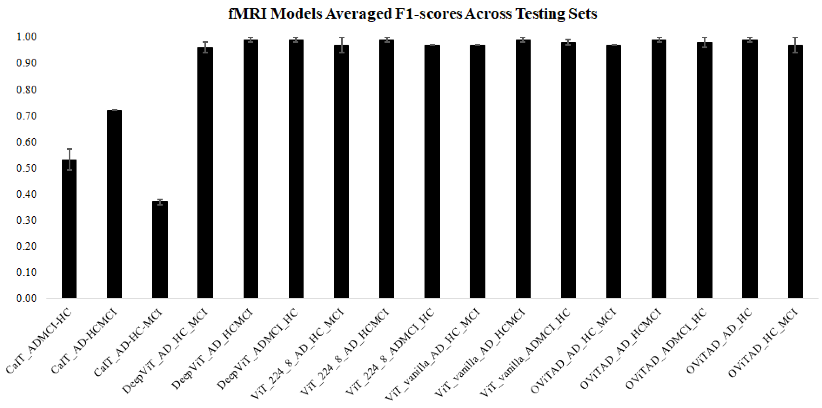
| OViTAD - fMRI | * First Vision Transformer for Alzheimer’s prediction using rs-fMRI * Aggressive fMRI preprocessing + 4D data decomposition to 2D * postprocessing to retrieve subject-level prediction |
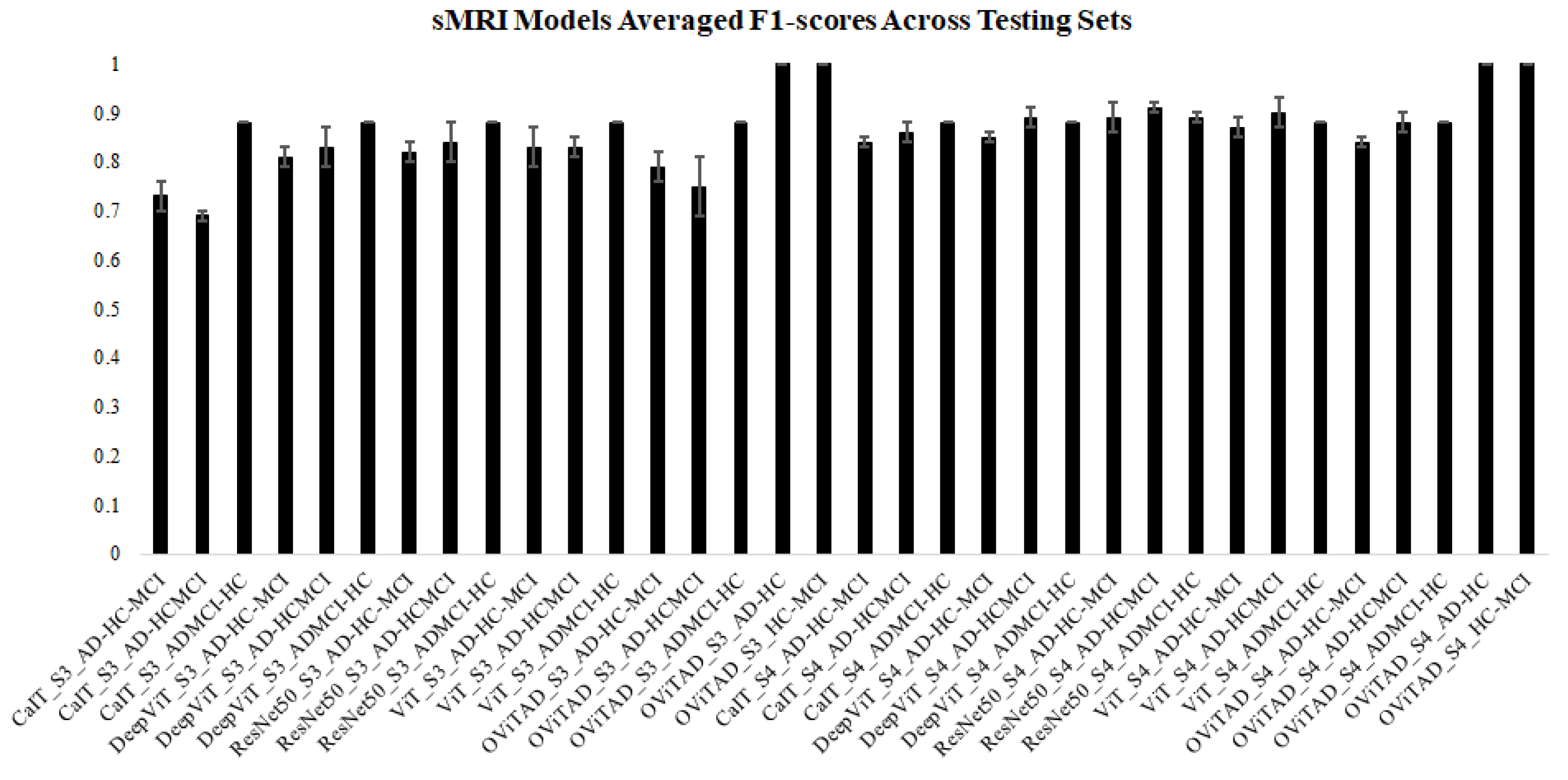
| OViTAD - MRI (Sigma = 3,4) | * First Vision Transformer for Alzheimer’s prediction using MRI * Aggressive fMRI preprocessing + 3D data decomposition to 2D * postprocessing to retrieve subject-level prediction |


References
- Lin, P.J.; D’Cruz, B.; Leech, A.A.; Neumann, P.J.; Sanon Aigbogun, M.; Oberdhan, D.; Lavelle, T.A. Family and caregiver spillover effects in cost-utility analyses of Alzheimer’s disease interventions. Pharmacoeconomics 2019, 37, 597–608. [Google Scholar] [CrossRef] [PubMed]
- Alzheimer’s Association. 2018 Alzheimer’s disease facts and figures. Alzheimer’s Dement. 2018, 14, 367–429. [Google Scholar] [CrossRef]
- Frisoni, G.B.; Boccardi, M.; Barkhof, F.; Blennow, K.; Cappa, S.; Chiotis, K.; Démonet, J.F.; Garibotto, V.; Giannakopoulos, P.; Gietl, A.; et al. Strategic roadmap for an early diagnosis of Alzheimer’s disease based on biomarkers. Lancet Neurol. 2017, 16, 661–676. [Google Scholar] [CrossRef]
- Rasmussen, J.; Langerman, H. Alzheimer’s disease–why we need early diagnosis. Degener. Neurol. Neuromuscul. Dis. 2019, 9, 123. [Google Scholar] [CrossRef]
- Fitzpatrick, A.W.; Falcon, B.; He, S.; Murzin, A.G.; Murshudov, G.; Garringer, H.J.; Crowther, R.A.; Ghetti, B.; Goedert, M.; Scheres, S.H. Cryo-EM structures of tau filaments from Alzheimer’s disease. Nature 2017, 547, 185–190. [Google Scholar] [CrossRef]
- Mazure, C.M.; Swendsen, J. Sex differences in Alzheimer’s disease and other dementias. Lancet Neurol. 2016, 15, 451. [Google Scholar] [CrossRef]
- Murphy, M.C.; Jones, D.T.; Jack, C.R., Jr.; Glaser, K.J.; Senjem, M.L.; Manduca, A.; Felmlee, J.P.; Carter, R.E.; Ehman, R.L.; Huston, J., III. Regional brain stiffness changes across the Alzheimer’s disease spectrum. Neuroimage Clin. 2016, 10, 283–290. [Google Scholar] [CrossRef]
- Gillis, C.; Mirzaei, F.; Potashman, M.; Ikram, M.A.; Maserejian, N. The incidence of mild cognitive impairment: A systematic review and data synthesis. Alzheimer’s Dementia: Diagn. Assess. Dis. Monit. 2019, 11, 248–256. [Google Scholar] [CrossRef] [PubMed]
- Cabeza, R.; Albert, M.; Belleville, S.; Craik, F.I.; Duarte, A.; Grady, C.L.; Lindenberger, U.; Nyberg, L.; Park, D.C.; Reuter-Lorenz, P.A.; et al. Maintenance, reserve and compensation: The cognitive neuroscience of healthy ageing. Nat. Rev. Neurosci. 2018, 19, 701–710. [Google Scholar] [CrossRef] [PubMed]
- Petersen, R.C. Mild cognitive impairment. Contin. Lifelong Learn. Neurol. 2016, 22, 404. [Google Scholar]
- Anthony, M.; Lin, F. A systematic review for functional neuroimaging studies of cognitive reserve across the cognitive aging spectrum. Arch. Clin. Neuropsychol. 2018, 33, 937–948. [Google Scholar] [CrossRef] [PubMed]
- Mateos-Pérez, J.M.; Dadar, M.; Lacalle-Aurioles, M.; Iturria-Medina, Y.; Zeighami, Y.; Evans, A.C. Structural neuroimaging as clinical predictor: A review of machine learning applications. NeuroImage Clin. 2018, 20, 506–522. [Google Scholar] [CrossRef] [PubMed]
- Neale, N.; Padilla, C.; Fonseca, L.M.; Holland, T.; Zaman, S. Neuroimaging and other modalities to assess Alzheimer’s disease in Down syndrome. NeuroImage Clin. 2018, 17, 263–271. [Google Scholar] [CrossRef] [PubMed]
- Rathore, S.; Habes, M.; Iftikhar, M.A.; Shacklett, A.; Davatzikos, C. A review on neuroimaging-based classification studies and associated feature extraction methods for Alzheimer’s disease and its prodromal stages. NeuroImage 2017, 155, 530–548. [Google Scholar] [CrossRef]
- Vemuri, P.; Lesnick, T.G.; Przybelski, S.A.; Knopman, D.S.; Lowe, V.J.; Graff-Radford, J.; Roberts, R.O.; Mielke, M.M.; Machulda, M.M.; Petersen, R.C.; et al. Age, vascular health, and Alzheimer disease biomarkers in an elderly sample. Ann. Neurol. 2017, 82, 706–718. [Google Scholar] [CrossRef]
- Lindquist, M. Neuroimaging results altered by varying analysis pipelines, 2020. Nature 2020, 582, 36–37. [Google Scholar] [CrossRef]
- Wang, X.; Huang, W.; Su, L.; Xing, Y.; Jessen, F.; Sun, Y.; Shu, N.; Han, Y. Neuroimaging advances regarding subjective cognitive decline in preclinical Alzheimer’s disease. Mol. Neurodegener. 2020, 15, 1–27. [Google Scholar] [CrossRef]
- Hainc, N.; Federau, C.; Stieltjes, B.; Blatow, M.; Bink, A.; Stippich, C. The bright, artificial intelligence-augmented future of neuroimaging reading. Front. Neurol. 2017, 8, 489. [Google Scholar] [CrossRef] [PubMed]
- Jo, T.; Nho, K.; Saykin, A.J. Deep learning in Alzheimer’s disease: Diagnostic classification and prognostic prediction using neuroimaging data. Front. Aging Neurosci. 2019, 220. [Google Scholar] [CrossRef] [PubMed]
- Henschel, L.; Conjeti, S.; Estrada, S.; Diers, K.; Fischl, B.; Reuter, M. Fastsurfer-a fast and accurate deep learning based neuroimaging pipeline. NeuroImage 2020, 219, 117012. [Google Scholar] [CrossRef]
- Puranik, M.; Shah, H.; Shah, K.; Bagul, S. Intelligent Alzheimer’s detector using deep learning. In Proceedings of the 2018 Second International Conference on Intelligent Computing and Control Systems (ICICCS), Madurai, India, 14–15 June 2018; pp. 318–323. [Google Scholar]
- Bi, X.; Li, S.; Xiao, B.; Li, Y.; Wang, G.; Ma, X. Computer aided Alzheimer’s disease diagnosis by an unsupervised deep learning technology. Neurocomputing 2020, 392, 296–304. [Google Scholar] [CrossRef]
- Kazemi, Y.; Houghten, S. A deep learning pipeline to classify different stages of Alzheimer’s disease from fMRI data. In Proceedings of the 2018 IEEE Conference on Computational Intelligence in Bioinformatics and Computational Biology (CIBCB), St. Louis, MO, USA, 30 May–2 June 2018; pp. 1–8. [Google Scholar]
- Tang, Z.; Chuang, K.V.; DeCarli, C.; Jin, L.W.; Beckett, L.; Keiser, M.J.; Dugger, B.N. Interpretable classification of Alzheimer’s disease pathologies with a convolutional neural network pipeline. Nat. Commun. 2019, 10, 1–14. [Google Scholar] [CrossRef] [PubMed]
- Wen, J.; Thibeau-Sutre, E.; Diaz-Melo, M.; Samper-González, J.; Routier, A.; Bottani, S.; Dormont, D.; Durrleman, S.; Burgos, N.; Colliot, O.; et al. Convolutional neural networks for classification of Alzheimer’s disease: Overview and reproducible evaluation. Med. Image Anal. 2020, 63, 101694. [Google Scholar] [CrossRef] [PubMed]
- Liu, M.; Cheng, D.; Wang, K.; Wang, Y. Multi-modality cascaded convolutional neural networks for Alzheimer’s disease diagnosis. Neuroinformatics 2018, 16, 295–308. [Google Scholar] [CrossRef]
- Islam, J.; Zhang, Y. Brain MRI analysis for Alzheimer’s disease diagnosis using an ensemble system of deep convolutional neural networks. Brain Informatics 2018, 5, 1–14. [Google Scholar] [CrossRef] [PubMed]
- Song, T.A.; Chowdhury, S.R.; Yang, F.; Jacobs, H.; El Fakhri, G.; Li, Q.; Johnson, K.; Dutta, J. Graph convolutional neural networks for Alzheimer’s disease classification. In Proceedings of the 2019 IEEE 16th International Symposium on Biomedical Imaging (ISBI 2019), Venice, Italy, 8–11 April 2019; pp. 414–417. [Google Scholar]
- Sarraf, A.; Jalali, A.E.; Ghaffari, J. Recent Applications of Deep Learning Algorithms in Medical Image Analysis. Am. Acad. Sci. Res. J. Eng. Technol. Sci. 2020, 72, 58–66. [Google Scholar]
- Sarraf, A.; Azhdari, M.; Sarraf, S. A comprehensive review of deep learning architectures for computer vision applications. Am. Acad. Sci. Res. J. Eng. Technol. Sci. 2021, 77, 1–29. [Google Scholar]
- Janghel, R.; Rathore, Y. Deep convolution neural network based system for early diagnosis of Alzheimer’s disease. Irbm 2021, 42, 258–267. [Google Scholar] [CrossRef]
- Chen, S.; Zhang, J.; Wei, X.; Zhang, Q. Alzheimer’s Disease Classification Using Structural MRI Based on Convolutional Neural Networks. In Proceedings of the 2020 2nd International Conference on Big-data Service and Intelligent Computation, Johannesburg, South Africa, 28–30 April 2020; pp. 7–13. [Google Scholar]
- Albright, J.; Initiative, A.D.N. Forecasting the progression of Alzheimer’s disease using neural networks and a novel preprocessing algorithm. Alzheimer’s Dementia: Transl. Res. Clin. Interv. 2019, 5, 483–491. [Google Scholar] [CrossRef]
- Li, F.; Liu, M.; Initiative, A.D.N. A hybrid convolutional and recurrent neural network for hippocampus analysis in Alzheimer’s disease. J. Neurosci. Methods 2019, 323, 108–118. [Google Scholar] [CrossRef]
- Feng, C.; Elazab, A.; Yang, P.; Wang, T.; Zhou, F.; Hu, H.; Xiao, X.; Lei, B. Deep learning framework for Alzheimer’s disease diagnosis via 3D-CNN and FSBi-LSTM. IEEE Access 2019, 7, 63605–63618. [Google Scholar] [CrossRef]
- Dua, M.; Makhija, D.; Manasa, P.; Mishra, P. A CNN–RNN–LSTM based amalgamation for Alzheimer’s disease detection. J. Med. Biol. Eng. 2020, 40, 688–706. [Google Scholar] [CrossRef]
- Anwar, S.M.; Majid, M.; Qayyum, A.; Awais, M.; Alnowami, M.; Khan, M.K. Medical image analysis using convolutional neural networks: A review. J. Med. Syst. 2018, 42, 1–13. [Google Scholar] [CrossRef] [PubMed]
- Yao, G.; Lei, T.; Zhong, J. A review of convolutional-neural-network-based action recognition. Pattern Recognit. Lett. 2019, 118, 14–22. [Google Scholar] [CrossRef]
- Dhillon, A.; Verma, G.K. Convolutional neural network: A review of models, methodologies and applications to object detection. Prog. Artif. Intell. 2020, 9, 85–112. [Google Scholar] [CrossRef]
- Sornam, M.; Muthusubash, K.; Vanitha, V. A survey on image classification and activity recognition using deep convolutional neural network architecture. In Proceedings of the 2017 ninth international conference on advanced computing (ICoAC), Chennai, India, 14–16 December 2017; pp. 121–126. [Google Scholar]
- Sultana, F.; Sufian, A.; Dutta, P. Evolution of image segmentation using deep convolutional neural network: A survey. Knowl.-Based Syst. 2020, 201, 106062. [Google Scholar] [CrossRef]
- Ebrahimighahnavieh, M.A.; Luo, S.; Chiong, R. Deep learning to detect Alzheimer’s disease from neuroimaging: A systematic literature review. Comput. Methods Programs Biomed. 2020, 187, 105242. [Google Scholar] [CrossRef]
- Altinkaya, E.; Polat, K.; Barakli, B. Detection of Alzheimer’s disease and dementia states based on deep learning from MRI images: A comprehensive review. J. Inst. Electron. Comput. 2020, 1, 39–53. [Google Scholar]
- Murn, L.; Blasi, S.; Smeaton, A.F.; O’Connor, N.E.; Mrak, M. Interpreting CNN for low complexity learned sub-pixel motion compensation in video coding. In Proceedings of the 2020 IEEE International Conference on Image Processing (ICIP), Abu Dhabi, United Arab Emirates, 25–28 October 2020; pp. 798–802. [Google Scholar]
- You, J.; Korhonen, J. Transformer for image quality assessment. In Proceedings of the 2021 IEEE International Conference on Image Processing (ICIP), Anchorage, AK, USA, 19–22 September 2021; pp. 1389–1393. [Google Scholar]
- Li, N.; Liu, S.; Liu, Y.; Zhao, S.; Liu, M. Neural speech synthesis with transformer network. In Proceedings of the Proceedings of the AAAI Conference on Artificial Intelligence, Honolulu, HI, USA, 27 January–1 February 2019; Volume 33, pp. 6706–6713. [Google Scholar]
- Haller, S.; Lovblad, K.O.; Giannakopoulos, P. Principles of classification analyses in mild cognitive impairment (MCI) and Alzheimer disease. J. Alzheimer’s Dis. 2011, 26, 389–394. [Google Scholar] [CrossRef]
- Dukart, J.; Mueller, K.; Barthel, H.; Villringer, A.; Sabri, O.; Schroeter, M.L.; Initiative, A.D.N. Meta-analysis based SVM classification enables accurate detection of Alzheimer’s disease across different clinical centers using FDG-PET and MRI. Psychiatry Res. Neuroimaging 2013, 212, 230–236. [Google Scholar] [CrossRef]
- Suk, H.I.; Lee, S.W.; Shen, D.; Initiative, A.D.N. Hierarchical feature representation and multimodal fusion with deep learning for AD/MCI diagnosis. NeuroImage 2014, 101, 569–582. [Google Scholar] [CrossRef] [PubMed]
- Zhu, X.; Suk, H.I.; Lee, S.W.; Shen, D. Canonical feature selection for joint regression and multi-class identification in Alzheimer’s disease diagnosis. Brain Imaging Behav. 2016, 10, 818–828. [Google Scholar] [CrossRef] [PubMed]
- Rieke, J.; Eitel, F.; Weygandt, M.; Haynes, J.D.; Ritter, K. Visualizing convolutional networks for MRI-based diagnosis of Alzheimer’s disease. In Understanding and Interpreting Machine Learning in Medical Image Computing Applications; Springer: Berlin, Germany, 2018; pp. 24–31. [Google Scholar]
- Farooq, A.; Anwar, S.; Awais, M.; Rehman, S. A deep CNN based multi-class classification of Alzheimer’s disease using MRI. In Proceedings of the 2017 IEEE International Conference on Imaging systems and techniques (IST), Beijing, China, 18–20 October 2017; pp. 1–6. [Google Scholar]
- Long, X.; Chen, L.; Jiang, C.; Zhang, L.; Initiative, A.D.N. Prediction and classification of Alzheimer disease based on quantification of MRI deformation. PLoS ONE 2017, 12, e0173372. [Google Scholar] [CrossRef] [PubMed]
- Sarraf, S.; DeSouza, D.D.; Anderson, J.; Tofighi, G. DeepAD: Alzheimer’s disease classification via deep convolutional neural networks using MRI and fMRI. BioRxiv 2017, 070441. [Google Scholar]
- Wang, S.; Wang, H.; Shen, Y.; Wang, X. Automatic recognition of mild cognitive impairment and alzheimers disease using ensemble based 3d densely connected convolutional networks. In Proceedings of the 2018 17th IEEE International conference on machine learning and applications (ICMLA), Orlando, FL, USA, 17–20 December 2018; pp. 517–523. [Google Scholar]
- Khvostikov, A.; Aderghal, K.; Benois-Pineau, J.; Krylov, A.; Catheline, G. 3D CNN-based classification using sMRI and MD-DTI images for Alzheimer disease studies. arXiv 2018, arXiv:1801.05968. [Google Scholar]
- Hosseini-Asl, E.; Keynton, R.; El-Baz, A. Alzheimer’s disease diagnostics by adaptation of 3D convolutional network. In Proceedings of the 2016 IEEE international conference on image processing (ICIP), Phoenix, AZ, USA, 25–28 September 2016; pp. 126–130. [Google Scholar]
- Sarraf, S.; Desouza, D.D.; Anderson, J.A.; Saverino, C. MCADNNet: Recognizing stages of cognitive impairment through efficient convolutional fMRI and MRI neural network topology models. IEEE Access 2019, 7, 155584–155600. [Google Scholar] [CrossRef]
- Soliman, S.A.; Hussein, R.R.; El-Dahshan, E.S.A.; Salem, A.B.M. Intelligent Algorithms for the Diagnosis of Alzheimer’s Disease. In Innovative Smart Healthcare and Bio-Medical Systems; CRC Press: Boca Raton, FL, USA, 2020; pp. 51–86. [Google Scholar]
- Soliman, S.A.; El-Sayed, A.; Salem, A.B.M. Predicting Alzheimer’s Disease with 3D Convolutional Neural Networks. Int. J. Appl. Fuzzy Sets Artif. Intell. 2020, 10, 125–146. [Google Scholar]
- Duc, N.T.; Ryu, S.; Qureshi, M.N.I.; Choi, M.; Lee, K.H.; Lee, B. 3D-deep learning based automatic diagnosis of Alzheimer’s disease with joint MMSE prediction using resting-state fMRI. Neuroinformatics 2020, 18, 71–86. [Google Scholar] [CrossRef]
- Li, W.; Lin, X.; Chen, X. Detecting Alzheimer’s disease Based on 4D fMRI: An exploration under deep learning framework. Neurocomputing 2020, 388, 280–287. [Google Scholar] [CrossRef]
- Ramzan, F.; Khan, M.U.G.; Rehmat, A.; Iqbal, S.; Saba, T.; Rehman, A.; Mehmood, Z. A deep learning approach for automated diagnosis and multi-class classification of Alzheimer’s disease stages using resting-state fMRI and residual neural networks. J. Med. Syst. 2020, 44, 1–16. [Google Scholar] [CrossRef]
- Sarraf, S.; Tofighi, G. Deep learning-based pipeline to recognize Alzheimer’s disease using fMRI data. In Proceedings of the 2016 future technologies conference (FTC), San Francisco, CA, USA, 6–7 December 2016; pp. 816–820. [Google Scholar]
- Cheng, D.; Liu, M. Combining convolutional and recurrent neural networks for Alzheimer’s disease diagnosis using PET images. In Proceedings of the 2017 IEEE International Conference on Imaging Systems and Techniques (IST), Beijing, China, 18–20 October 2017; pp. 1–5. [Google Scholar]
- Hong, X.; Lin, R.; Yang, C.; Zeng, N.; Cai, C.; Gou, J.; Yang, J. Predicting Alzheimer’s disease using LSTM. IEEE Access 2019, 7, 80893–80901. [Google Scholar] [CrossRef]
- Wang, T.; Qiu, R.G.; Yu, M. Predictive modeling of the progression of Alzheimer’s disease with recurrent neural networks. Sci. Rep. 2018, 8, 1–12. [Google Scholar] [CrossRef] [PubMed]
- Sethi, M.; Ahuja, S.; Rani, S.; Bawa, P.; Zaguia, A. Classification of Alzheimer’s Disease Using Gaussian-Based Bayesian Parameter Optimization for Deep Convolutional LSTM Network. Comput. Math. Methods Med. 2021, 2021, 4186666. [Google Scholar] [CrossRef] [PubMed]
- Cui, R.; Liu, M.; Li, G. Longitudinal analysis for Alzheimer’s disease diagnosis using RNN. In Proceedings of the 2018 IEEE 15th International Symposium on Biomedical Imaging (ISBI 2018), Washington, DC, USA, 4–7 April 2018; pp. 1398–1401. [Google Scholar]
- Bubu, O.M.; Pirraglia, E.; Andrade, A.G.; Sharma, R.A.; Gimenez-Badia, S.; Umasabor-Bubu, O.Q.; Hogan, M.M.; Shim, A.M.; Mukhtar, F.; Sharma, N.; et al. Obstructive sleep apnea and longitudinal Alzheimer’s disease biomarker changes. Sleep 2019, 42, zsz048. [Google Scholar] [CrossRef]
- Benoit, J.S.; Chan, W.; Piller, L.; Doody, R. Longitudinal sensitivity of Alzheimer’s disease severity staging. Am. J. Alzheimer’s Dis. Other Dementias® 2020, 35, 1533317520918719. [Google Scholar] [CrossRef]
- Jabason, E.; Ahmad, M.O.; Swamy, M. Hybrid Feature Fusion Using RNN and Pre-trained CNN for Classification of Alzheimer’s Disease (Poster). In Proceedings of the 2019 22th International Conference on Information Fusion (FUSION), Ottawa, ON, Canada, 2–5 July 2019; pp. 1–4. [Google Scholar]
- Song, J.; Zheng, J.; Li, P.; Lu, X.; Zhu, G.; Shen, P. An effective multimodal image fusion method using MRI and PET for Alzheimer’s disease diagnosis. Front. Digit. Health 2021, 3, 19. [Google Scholar] [CrossRef]
- Gupta, Y.; Kim, J.I.; Kim, B.C.; Kwon, G.R. Classification and graphical analysis of Alzheimer’s disease and its prodromal stage using multimodal features from structural, diffusion, and functional neuroimaging data and the APOE genotype. Front. Aging Neurosci. 2020, 12, 238. [Google Scholar] [CrossRef]
- Thushara, A.; Amma, C.U.; John, A.; Saju, R. Multimodal MRI Based Classification and Prediction of Alzheimer’s Disease Using Random Forest Ensemble. In Proceedings of the 2020 Advanced Computing and Communication Technologies for High Performance Applications (ACCTHPA), Cochin, India, 2–4 July 2020; pp. 249–256. [Google Scholar]
- Liu, M.; Cheng, D.; Yan, W.; Initiative, A.D.N. Classification of Alzheimer’s disease by combination of convolutional and recurrent neural networks using FDG-PET images. Front. Neuroinformatics 2018, 12, 35. [Google Scholar] [CrossRef] [PubMed]
- Yuen, S.C.; Liang, X.; Zhu, H.; Jia, Y.; Leung, S.W. Prediction of differentially expressed microRNAs in blood as potential biomarkers for Alzheimer’s disease by meta-analysis and adaptive boosting ensemble learning. Alzheimer’s Res. Ther. 2021, 13, 1–30. [Google Scholar] [CrossRef] [PubMed]
- Kim, J.; Park, Y.; Park, S.; Jang, H.; Kim, H.J.; Na, D.L.; Lee, H.; Seo, S.W. Prediction of tau accumulation in prodromal Alzheimer’s disease using an ensemble machine learning approach. Sci. Rep. 2021, 11, 1–8. [Google Scholar] [CrossRef]
- Hu, D. An introductory survey on attention mechanisms in NLP problems. In Proceedings of the Proceedings of SAI Intelligent Systems Conference, London, UK, 5–6 September 2019; pp. 432–448. [Google Scholar]
- Letarte, G.; Paradis, F.; Giguère, P.; Laviolette, F. Importance of self-attention for sentiment analysis. In Proceedings of the Proceedings of the 2018 EMNLP Workshop BlackboxNLP: Analyzing and Interpreting Neural Networks for NLP, Brussels, Belgium, 1 November 2018; pp. 267–275. [Google Scholar]
- Roshanzamir, A.; Aghajan, H.; Soleymani Baghshah, M. Transformer-based deep neural network language models for Alzheimer’s disease risk assessment from targeted speech. BMC Med. Informatics Decis. Mak. 2021, 21, 1–14. [Google Scholar] [CrossRef] [PubMed]
- Sarasua, I.; Pölsterl, S.; Wachinger, C.; Neuroimaging, A.D. TransforMesh: A Transformer Network for Longitudinal Modeling of Anatomical Meshes. In Proceedings of the International Workshop on Machine Learning in Medical Imaging, Strasbourg, France, 27 September 2021; pp. 209–218. [Google Scholar]
- Wang, S.; Zhuang, Z.; Xuan, K.; Qian, D.; Xue, Z.; Xu, J.; Liu, Y.; Chai, Y.; Zhang, L.; Wang, Q.; et al. 3DMeT: 3D Medical Image Transformer for Knee Cartilage Defect Assessment. In Proceedings of the International Workshop on Machine Learning in Medical Imaging, Strasbourg, France, 27 September 2021; pp. 347–355. [Google Scholar]
- Jack, C.R., Jr.; Bernstein, M.A.; Fox, N.C.; Thompson, P.; Alexander, G.; Harvey, D.; Borowski, B.; Britson, P.J.; Whitwell, J.L.; Ward, C.; et al. The Alzheimer’s disease neuroimaging initiative (ADNI): MRI methods. J. Magn. Reson. Imaging Off. J. Int. Soc. Magn. Reson. Med. 2008, 27, 685–691. [Google Scholar] [CrossRef]
- Churchill, N.W.; Spring, R.; Afshin-Pour, B.; Dong, F.; Strother, S.C. An automated, adaptive framework for optimizing preprocessing pipelines in task-based functional MRI. PLoS ONE 2015, 10, e0131520. [Google Scholar] [CrossRef] [PubMed]
- Churchill, N.W.; Oder, A.; Abdi, H.; Tam, F.; Lee, W.; Thomas, C.; Ween, J.E.; Graham, S.J.; Strother, S.C. Optimizing preprocessing and analysis pipelines for single-subject fMRI. I. Standard temporal motion and physiological noise correction methods. Hum. Brain Mapp. 2012, 33, 609–627. [Google Scholar] [CrossRef] [PubMed]
- Li, X.; Morgan, P.S.; Ashburner, J.; Smith, J.; Rorden, C. The first step for neuroimaging data analysis: DICOM to NIfTI conversion. J. Neurosci. Methods 2016, 264, 47–56. [Google Scholar] [CrossRef]
- Smith, S.M. Fast robust automated brain extraction. Hum. Brain Mapp. 2002, 17, 143–155. [Google Scholar] [CrossRef]
- Jenkinson, M.; Bannister, P.; Brady, M.; Smith, S. Improved optimization for the robust and accurate linear registration and motion correction of brain images. Neuroimage 2002, 17, 825–841. [Google Scholar] [CrossRef]
- Fonov, V.; Evans, A.C.; Botteron, K.; Almli, C.R.; McKinstry, R.C.; Collins, D.L.; the Brain Development Cooperative Group. Unbiased average age-appropriate atlases for pediatric studies. Neuroimage 2011, 54, 313–327. [Google Scholar] [CrossRef]
- Smith, S.M.; Jenkinson, M.; Woolrich, M.W.; Beckmann, C.F.; Behrens, T.E.; Johansen-Berg, H.; Bannister, P.R.; De Luca, M.; Drobnjak, I.; Flitney, D.E.; et al. Advances in functional and structural MR image analysis and implementation as FSL. Neuroimage 2004, 23, S208–S219. [Google Scholar] [CrossRef]
- Scarpazza, C.; Tognin, S.; Frisciata, S.; Sartori, G.; Mechelli, A. False positive rates in Voxel-based Morphometry studies of the human brain: Should we be worried? Neurosci. Biobehav. Rev. 2015, 52, 49–55. [Google Scholar] [CrossRef]
- Mikl, M.; Mareček, R.; Hluštík, P.; Pavlicová, M.; Drastich, A.; Chlebus, P.; Brázdil, M.; Krupa, P. Effects of spatial smoothing on fMRI group inferences. Magn. Reson. Imaging 2008, 26, 490–503. [Google Scholar] [CrossRef]
- Vaswani, A.; Shazeer, N.; Parmar, N.; Uszkoreit, J.; Jones, L.; Gomez, A.N.; Kaiser, Ł.; Polosukhin, I. Attention is all you need. Adv. Neural Inf. Process. Syst. 2017, 30, 1–11. [Google Scholar]
- Dosovitskiy, A.; Beyer, L.; Kolesnikov, A.; Weissenborn, D.; Zhai, X.; Unterthiner, T.; Dehghani, M.; Minderer, M.; Heigold, G.; Gelly, S.; et al. An image is worth 16x16 words: Transformers for image recognition at scale. arXiv 2020, arXiv:2010.11929. [Google Scholar]
- Zhou, D.; Kang, B.; Jin, X.; Yang, L.; Lian, X.; Jiang, Z.; Hou, Q.; Feng, J. Deepvit: Towards deeper vision transformer. arXiv 2021, arXiv:2103.11886. [Google Scholar]
- Touvron, H.; Cord, M.; Sablayrolles, A.; Synnaeve, G.; Jégou, H. Going deeper with image transformers. In Proceedings of the Proceedings of the IEEE/CVF International Conference on Computer Vision, Montreal, QC, Canada, 10–17 October 2021; pp. 32–42. [Google Scholar]
- Alakörkkö, T.; Saarimäki, H.; Glerean, E.; Saramäki, J.; Korhonen, O. Effects of spatial smoothing on functional brain networks. Eur. J. Neurosci. 2017, 46, 2471–2480. [Google Scholar] [CrossRef]
- Chen, Z.; Calhoun, V. Effect of spatial smoothing on task fMRI ICA and functional connectivity. Front. Neurosci. 2018, 12, 15. [Google Scholar] [CrossRef] [PubMed]
- Lin, W.; Tong, T.; Gao, Q.; Guo, D.; Du, X.; Yang, Y.; Guo, G.; Xiao, M.; Du, M.; Qu, X.; et al. Convolutional neural networks-based MRI image analysis for the Alzheimer’s disease prediction from mild cognitive impairment. Front. Neurosci. 2018, 777. [Google Scholar] [CrossRef]
- Dimitriadis, S.I.; Liparas, D.; Initiative, A.D.N. How random is the random forest? Random forest algorithm on the service of structural imaging biomarkers for Alzheimer’s disease: From Alzheimer’s disease neuroimaging initiative (ADNI) database. Neural Regen. Res. 2018, 13, 962. [Google Scholar] [CrossRef]
- Kruthika, K.; Maheshappa, H.; Initiative, A.D.N. Multistage classifier-based approach for Alzheimer’s disease prediction and retrieval. Informatics Med. Unlocked 2019, 14, 34–42. [Google Scholar] [CrossRef]
- Spasov, S.; Passamonti, L.; Duggento, A.; Lio, P.; Toschi, N.; Initiative, A.D.N. A parameter-efficient deep learning approach to predict conversion from mild cognitive impairment to Alzheimer’s disease. Neuroimage 2019, 189, 276–287. [Google Scholar] [CrossRef]
- Basaia, S.; Agosta, F.; Wagner, L.; Canu, E.; Magnani, G.; Santangelo, R.; Filippi, M.; Initiative, A.D.N. Automated classification of Alzheimer’s disease and mild cognitive impairment using a single MRI and deep neural networks. NeuroImage Clin. 2019, 21, 101645. [Google Scholar] [CrossRef] [PubMed]
- Abrol, A.; Bhattarai, M.; Fedorov, A.; Du, Y.; Plis, S.; Calhoun, V.; Initiative, A.D.N. Deep residual learning for neuroimaging: An application to predict progression to Alzheimer’s disease. J. Neurosci. Methods 2020, 339, 108701. [Google Scholar] [CrossRef]
- Shao, W.; Peng, Y.; Zu, C.; Wang, M.; Zhang, D.; Initiative, A.D.N. Hypergraph based multi-task feature selection for multimodal classification of Alzheimer’s disease. Comput. Med. Imaging Graph. 2020, 80, 101663. [Google Scholar] [CrossRef]
- Alinsaif, S.; Lang, J.; Initiative, A.D.N. 3D shearlet-based descriptors combined with deep features for the classification of Alzheimer’s disease based on MRI data. Comput. Biol. Med. 2021, 138, 104879. [Google Scholar] [CrossRef]
- Hojjati, S.H.; Ebrahimzadeh, A.; Khazaee, A.; Babajani-Feremi, A.; Initiative, A.D.N. Predicting conversion from MCI to AD by integrating rs-fMRI and structural MRI. Comput. Biol. Med. 2018, 102, 30–39. [Google Scholar] [CrossRef]
- Cui, R.; Liu, M.; Initiative, A.D.N. RNN-based longitudinal analysis for diagnosis of Alzheimer’s disease. Comput. Med. Imaging Graph. 2019, 73, 1–10. [Google Scholar] [CrossRef]
- Amoroso, N.; Diacono, D.; Fanizzi, A.; La Rocca, M.; Monaco, A.; Lombardi, A.; Guaragnella, C.; Bellotti, R.; Tangaro, S.; Initiative, A.D.N.; et al. Deep learning reveals Alzheimer’s disease onset in MCI subjects: Results from an international challenge. J. Neurosci. Methods 2018, 302, 3–9. [Google Scholar] [CrossRef] [PubMed]
- Buvaneswari, P.; Gayathri, R. Detection and Classification of Alzheimer’s disease from cognitive impairment with resting-state fMRI. Neural Comput. Appl. 2021, 1, 1–16. [Google Scholar] [CrossRef]


| Modality | Total | Group | Participant | Female | Age | Male | Age | MMSE |
|---|---|---|---|---|---|---|---|---|
| rs-fMRI | 284 | AD | 54 | 27 | 80.96 ± 4.64 | 27 | 79.0 ± 2.74 | 22.70 ± 2.10 |
| HC | 99 | 49 | 79.78 ± 4.76 | 50 | 82.57 ± 3.88 | 28.82 ± 1.35 | ||
| MCI | 131 | 66 | 79.15 ± 3.09 | 65 | 79.72 ± 4.84 | 26.53 ± 2.51 | ||
| MRI | 1460 | AD | 577 | 232 | 80.98 ± 4.65 | 345 | 81.27 ± 4.08 | 23.07 ± 2.06 |
| HC | 108 | 51 | 79.37 ± 3.54 | 57 | 80.81 ± 4.42 | 28.81 ± 1.35 | ||
| MCI | 775 | 265 | 80.28 ± 3.31 | 510 | 81.61 ± 4.15 | 26.53 ± 2.09 |
| Model | Dataset | Precision | Recall | F1-Score | Accuracy |
|---|---|---|---|---|---|
| CaIT_ADMCI-HC | Val | 0.53 ± 0.14 | 0.68 ± 0.02 | 0.57 ± 0.07 | 0.68 ± 0.02 |
| Test | 0.54 ± 0.21 | 0.66 ± 0.02 | 0.53 ± 0.04 | 0.66 ± 0.02 | |
| CaIT_AD-HCMCI | Val | 0.66 ± 0 | 0.81 ± 0 | 0.73 ± 0 | 0.81 ± 0 |
| Test | 0.65 ± 0 | 0.81 ± 0 | 0.72 ± 0 | 0.81 ± 0 | |
| CaIT_AD-HC-MCI | Val | 0.4 ± 0.14 | 0.54 ± 0.06 | 0.43 ± 0.11 | 0.54 ± 0.06 |
| Test | 0.37 ± 0.01 | 0.46 ± 0.02 | 0.37 ± 0.01 | 0.46 ± 0.02 | |
| DeepViT_AD_HC_MCI | Val | 1 ± 0 | 1 ± 0 | 1 ± 0 | 1 ± 0 |
| Test | 0.96 ± 0.02 | 0.96 ± 0.02 | 0.96 ± 0.02 | 0.96 ± 0.02 | |
| DeepViT_AD_HCMCI | Val | 0.99 ± 0.02 | 0.99 ± 0.02 | 0.99 ± 0.02 | 0.99 ± 0.02 |
| Test | 0.99 ± 0.02 | 0.99 ± 0.02 | 0.99 ± 0.02 | 0.99 ± 0.02 | |
| DeepViT_ADMCI_HC | Val | 1 ± 0 | 1 ± 0 | 1 ± 0 | 1 ± 0 |
| Test | 0.99 ± 0.02 | 0.99 ± 0.02 | 0.99 ± 0.02 | 0.99 ± 0.02 | |
| ViT_224_8_AD_HC_MCI | Val | 0.99 ± 0.02 | 0.99 ± 0.02 | 0.99 ± 0.02 | 0.99 ± 0.02 |
| Test | 0.97 ± 0.03 | 0.97 ± 0.03 | 0.97 ± 0.03 | 0.97 ± 0.03 | |
| ViT_224_8_AD_HCMCI | Val | 1 ± 0 | 1 ± 0 | 1 ± 0 | 1 ± 0 |
| Test | 0.99 ± 0.02 | 0.99 ± 0.02 | 0.99 ± 0.02 | 0.99 ± 0.02 | |
| ViT_224_8_ADMCI_HC | Val | 1 ± 0 | 1 ± 0 | 1 ± 0 | 1 ± 0 |
| Test | 0.97 ± 0 | 0.97 ± 0 | 0.97 ± 0 | 0.97 ± 0 | |
| ViT_vanilla_AD_HC_MCI | Val | 0.99 ± 0.02 | 0.99 ± 0.02 | 0.99 ± 0.02 | 0.99 ± 0.02 |
| Test | 0.97 ± 0 | 0.97 ± 0 | 0.97 ± 0 | 0.97 ± 0 | |
| ViT_vanilla_AD_HCMCI | Val | 1 ± 0 | 1 ± 0 | 1 ± 0 | 1 ± 0 |
| Test | 0.99 ± 0.02 | 0.99 ± 0.02 | 0.99 ± 0.02 | 0.99 ± 0.02 | |
| ViT_vanilla_ADMCI_HC | Val | 1 ± 0 | 1 ± 0 | 1 ± 0 | 1 ± 0 |
| Test | 0.98 ± 0.02 | 0.98 ± 0.02 | 0.98 ± 0.02 | 0.98 ± 0.02 | |
| OViTAD_AD_HC_MCI | Val | 0.99 ± 0.02 | 0.99 ± 0.02 | 0.99 ± 0.02 | 0.99 ± 0.02 |
| Test | 0.97 ± 0 | 0.97 ± 0 | 0.97 ± 0 | 0.97 ± 0 | |
| OViTAD_AD_HCMCI | Val | 0.99 ± 0.02 | 0.99 ± 0.02 | 0.99 ± 0.02 | 0.99 ± 0.02 |
| Test | 0.99 ± 0.02 | 0.99 ± 0.02 | 0.99 ± 0.02 | 0.99 ± 0.02 | |
| OViTAD_ADMCI_HC | Val | 1 ± 0 | 1 ± 0 | 1 ± 0 | 1 ± 0 |
| Test | 0.98 ± 0.02 | 0.98 ± 0.02 | 0.98 ± 0.02 | 0.98 ± 0.02 | |
| OViTAD_AD_HC | Val | 1 ± 0 | 1 ± 0 | 1 ± 0 | 1 ± 0 |
| Test | 0.99 ± 0.02 | 0.99 ± 0.02 | 0.99 ± 0.02 | 0.99 ± 0.02 | |
| OViTAD_HC_MCI | Val | 1 ± 0 | 1 ± 0 | 1 ± 0 | 1 ± 0 |
| Test | 0.97 ± 0.03 | 0.97 ± 0.03 | 0.97 ± 0.03 | 0.97 ± 0.03 |
| Model | Dataset | Precision | Recall | F1-Score | Accuracy |
|---|---|---|---|---|---|
| CaIT_S3_AD-HC-MCI | Val | 0.74 ± 0.02 | 0.8 ± 0.02 | 0.77 ± 0.02 | 0.8 ± 0.02 |
| Test | 0.71 ± 0.02 | 0.77 ± 0.03 | 0.73 ± 0.03 | 0.77 ± 0.03 | |
| CaIT_S3_AD-HCMCI | Val | 0.72 ± 0.02 | 0.72 ± 0.03 | 0.7 ± 0.03 | 0.72 ± 0.03 |
| Test | 0.71 ± 0.02 | 0.7 ± 0.01 | 0.69 ± 0.01 | 0.7 ± 0.01 | |
| CaIT_S3_ADMCI-HC | Val | 0.87 ± 0 | 0.93 ± 0 | 0.9 ± 0 | 0.93 ± 0 |
| Test | 0.85 ± 0 | 0.92 ± 0 | 0.88 ± 0 | 0.92 ± 0 | |
| DeepViT_S3_AD-HC-MCI | Val | 0.81 ± 0.06 | 0.85 ± 0.03 | 0.82 ± 0.04 | 0.85 ± 0.03 |
| Test | 0.77 ± 0.02 | 0.84 ± 0.02 | 0.81 ± 0.02 | 0.84 ± 0.02 | |
| DeepViT_S3_AD-HCMCI | Val | 0.84 ± 0.04 | 0.84 ± 0.05 | 0.84 ± 0.05 | 0.84 ± 0.05 |
| Test | 0.83 ± 0.04 | 0.83 ± 0.04 | 0.83 ± 0.04 | 0.83 ± 0.04 | |
| DeepViT_S3_ADMCI-HC | Val | 0.87 ± 0 | 0.93 ± 0 | 0.9 ± 0 | 0.93 ± 0 |
| Test | 0.85 ± 0 | 0.92 ± 0 | 0.88 ± 0 | 0.92 ± 0 | |
| ResNet50_S3_AD-HC-MCI | Val | 0.85 ± 0.09 | 0.86 ± 0.05 | 0.84 ± 0.06 | 0.86 ± 0.05 |
| Test | 0.83 ± 0.06 | 0.85 ± 0.02 | 0.82 ± 0.02 | 0.85 ± 0.02 | |
| ResNet50_S3_AD-HCMCI | Val | 0.84 ± 0.01 | 0.84 ± 0.01 | 0.84 ± 0.01 | 0.84 ± 0.01 |
| Test | 0.84 ± 0.04 | 0.84 ± 0.04 | 0.84 ± 0.04 | 0.84 ± 0.04 | |
| ResNet50_S3_ADMCI-HC | Val | 0.87 ± 0 | 0.93 ± 0 | 0.9 ± 0 | 0.93 ± 0 |
| Test | 0.85 ± 0 | 0.92 ± 0 | 0.88 ± 0 | 0.92 ± 0 | |
| ViT_S3_AD-HC-MCI | Val | 0.84 ± 0.05 | 0.88 ± 0.02 | 0.85 ± 0.03 | 0.88 ± 0.02 |
| Test | 0.84 ± 0.08 | 0.85 ± 0.03 | 0.83 ± 0.04 | 0.85 ± 0.03 | |
| ViT_S3_AD-HCMCI | Val | 0.84 ± 0.01 | 0.84 ± 0.01 | 0.83 ± 0.02 | 0.84 ± 0.01 |
| Test | 0.84 ± 0.03 | 0.83 ± 0.02 | 0.83 ± 0.02 | 0.83 ± 0.02 | |
| ViT_S3_ADMCI-HC | Val | 0.87 ± 0 | 0.93 ± 0 | 0.9 ± 0 | 0.93 ± 0 |
| Test | 0.85 ± 0 | 0.92 ± 0 | 0.88 ± 0 | 0.92 ± 0 | |
| OViTAD_S3_AD-HC-MCI | Val | 0.78 ± 0.02 | 0.84 ± 0.02 | 0.81 ± 0.02 | 0.84 ± 0.02 |
| Test | 0.75 ± 0.03 | 0.82 ± 0.03 | 0.79 ± 0.03 | 0.82 ± 0.03 | |
| OViTAD_S3_AD-HCMCI | Val | 0.79 ± 0.03 | 0.77 ± 0.05 | 0.75 ± 0.07 | 0.77 ± 0.05 |
| Test | 0.79 ± 0.02 | 0.77 ± 0.04 | 0.75 ± 0.06 | 0.77 ± 0.04 | |
| OViTAD_S3_ADMCI-HC | Val | 0.87 ± 0 | 0.93 ± 0 | 0.9 ± 0 | 0.93 ± 0 |
| Test | 0.85 ± 0 | 0.92 ± 0 | 0.88 ± 0 | 0.92 ± 0 | |
| OViTAD_S3_AD-HC | Val | 1 ± 0 | 1 ± 0 | 1 ± 0 | 1 ± 0 |
| Test | 1 ± 0 | 1 ± 0 | 1 ± 0 | 1 ± 0 | |
| OViTAD_S3_HC-MCI | Val | 1 ± 0 | 1 ± 0 | 1 ± 0 | 1 ± 0 |
| Test | 1 ± 0 | 1 ± 0 | 1 ± 0 | 1 ± 0 | |
| CaIT_S4_AD-HC-MCI | Val | 0.84 ± 0.03 | 0.9 ± 0.03 | 0.87 ± 0.03 | 0.9 ± 0.03 |
| Test | 0.81 ± 0.01 | 0.88 ± 0.01 | 0.84 ± 0.01 | 0.88 ± 0.01 | |
| CaIT_S4_AD-HCMCI | Val | 0.87 ± 0.02 | 0.87 ± 0.02 | 0.87 ± 0.02 | 0.87 ± 0.02 |
| Test | 0.86 ± 0.02 | 0.86 ± 0.02 | 0.86 ± 0.02 | 0.86 ± 0.02 | |
| CaIT_S4_ADMCI-HC | Val | 0.87 ± 0 | 0.93 ± 0 | 0.9 ± 0 | 0.93 ± 0 |
| Test | 0.85 ± 0 | 0.92 ± 0 | 0.88 ± 0 | 0.92 ± 0 | |
| DeepViT_S4_AD-HC-MCI | Val | 0.85 ± 0.01 | 0.91 ± 0.01 | 0.88 ± 0.01 | 0.91 ± 0.01 |
| Test | 0.82 ± 0.01 | 0.88 ± 0.01 | 0.85 ± 0.01 | 0.88 ± 0.01 | |
| DeepViT_S4_AD-HCMCI | Val | 0.91 ± 0.01 | 0.91 ± 0.01 | 0.91 ± 0.01 | 0.91 ± 0.01 |
| Test | 0.89 ± 0.02 | 0.89 ± 0.02 | 0.89 ± 0.02 | 0.89 ± 0.02 | |
| DeepViT_S4_ADMCI-HC | Val | 0.87 ± 0 | 0.93 ± 0 | 0.9 ± 0 | 0.93 ± 0 |
| Test | 0.85 ± 0 | 0.92 ± 0 | 0.88 ± 0 | 0.92 ± 0 | |
| ResNet50_S4_AD-HC-MCI | Val | 0.93 ± 0.01 | 0.93 ± 0.01 | 0.91 ± 0.01 | 0.93 ± 0.01 |
| Test | 0.89 ± 0.06 | 0.91 ± 0.02 | 0.89 ± 0.03 | 0.91 ± 0.02 | |
| ResNet50_S4_AD-HCMCI | Val | 0.93 ± 0 | 0.93 ± 0 | 0.93 ± 0 | 0.93 ± 0 |
| Test | 0.91 ± 0.01 | 0.91 ± 0.01 | 0.91 ± 0.01 | 0.91 ± 0.01 | |
| ResNet50_S4_ADMCI-HC | Val | 0.87 ± 0 | 0.93 ± 0 | 0.9 ± 0 | 0.93 ± 0 |
| Test | 0.87 ± 0.05 | 0.92 ± 0 | 0.89 ± 0.01 | 0.92 ± 0 | |
| ViT_S4_AD-HC-MCI | Val | 0.9 ± 0.06 | 0.91 ± 0.02 | 0.89 ± 0.02 | 0.91 ± 0.02 |
| Test | 0.88 ± 0.06 | 0.9 ± 0.02 | 0.87 ± 0.02 | 0.9 ± 0.02 | |
| ViT_S4_AD-HCMCI | Val | 0.91 ± 0 | 0.91 ± 0 | 0.91 ± 0 | 0.91 ± 0 |
| Test | 0.9 ± 0.03 | 0.9 ± 0.03 | 0.9 ± 0.03 | 0.9 ± 0.03 | |
| ViT_S4_ADMCI-HC | Val | 0.87 ± 0 | 0.93 ± 0 | 0.9 ± 0 | 0.93 ± 0 |
| Test | 0.85 ± 0 | 0.92 ± 0 | 0.88 ± 0 | 0.92 ± 0 | |
| OViTAD_S4_AD-HC-MCI | Val | 0.86 ± 0.06 | 0.9 ± 0.02 | 0.87 ± 0.03 | 0.9 ± 0.02 |
| Test | 0.81 ± 0.01 | 0.87 ± 0.01 | 0.84 ± 0.01 | 0.87 ± 0.01 | |
| OViTAD_S4_AD-HCMCI | Val | 0.9 ± 0 | 0.89 ± 0 | 0.89 ± 0 | 0.89 ± 0 |
| Test | 0.89 ± 0.02 | 0.88 ± 0.02 | 0.88 ± 0.02 | 0.88 ± 0.02 | |
| OViTAD_S4_ADMCI-HC | Val | 0.87 ± 0 | 0.93 ± 0 | 0.9 ± 0 | 0.93 ± 0 |
| Test | 0.85 ± 0 | 0.92 ± 0 | 0.88 ± 0 | 0.92 ± 0 | |
| OViTAD_S4_AD-HC | Val | 1 ± 0 | 1 ± 0 | 1 ± 0 | 1 ± 0 |
| Test | 1 ± 0 | 1 ± 0 | 1 ± 0 | 1 ± 0 | |
| OViTAD_S4_HC-MCI | Val | 1 ± 0 | 1 ± 0 | 1 ± 0 | 1 ± 0 |
| Test | 1 ± 0 | 1 ± 0 | 1 ± 0 | 1 ± 0 |
| Model | Input (Channel,x,y) | Params |
|---|---|---|
| CaIT | 3,224,224 | 120,707,075 |
| DeepViT | 3,224,224 | 53,532,867 |
| ViT-vanilla | 3,224,224 | 53,532,675 |
| ViT-224-8 | 3,224,224 | 40,949,763 |
| OViTAD | 3,56,56 | 38,406,147 |
| Reference | Modality | AD vs. HC vs. MCI | AD + MCI vs. HC | AD vs. MCI+HC | AD vs. HC | MCI vs. HC |
|---|---|---|---|---|---|---|
| Lin et al. 2018 [100] | MRI | - | - | - | 88.79% | - |
| Dimitriadis et al. 2018 [101] | MRI | 61.90% | - | - | - | - |
| Kruthika et al. 2019 [102] | MRI | 90.47% | - | - | - | - |
| Spasov et al. 2019 [103] | MRI + Clinical | - | - | - | - | 86% |
| Basaia et al. 2019 [104] | MRI | - | - | - | 98% | 87% |
| Abrol et al. 2020 [105] | MRI | 83.01% | - | - | - | - |
| Shao et al. 2020 [106] | MRI+PET | - | - | - | 92.51% | 82.53% |
| Alinsaif et al. 2021 [107] | MRI | - | 70.50% | - | 62.22% | - |
| Alinsaif et al. 2021 [107] | MRI | - | 91.61% | - | 92.78% | - |
| Ramzan et al. 2019 [63] | rs-fMRI | 97.92% | - | - | - | - |
| Hojjati et al. 2018 [108] | MRI + rs-fMRI | - | - | 93% | - | - |
| Cui et al. 2019 [109] | MRI | - | - | - | 91.33% | - |
| Amoroso et al. 2018 [110] | MRI | 38.80% | - | - | - | - |
| Buvaneswari et al. 2021 [111] | rs-fMRI | - | - | - | - | 79.15% |
| Duc et al. 2019 [61] | rs-fMRI+Clinical | - | - | - | 85.27% | - |
| OViTAD—fMRI | rs-fMRI | 0.97 ± 0 | 0.98 ± 0.02 | 0.99 ± 0.02 | 0.99 ± 0.02 | 0.97 ± 0.03 |
| OViTAD—MRI (Sigma = 3) | MRI | 0.9955% ± 0.0039 | 1 ± 0 | 0.9955 ± 0.0039 | 1 ± 0 | 1 ± 0 |
| OViTAD—MRI (Sigma = 4) | MRI | 0.9955% ± 0.0039 | 1 ± 0 | 0.9955 ± 0.0039 | 1 ± 0 | 1 ± 0 |
Disclaimer/Publisher’s Note: The statements, opinions and data contained in all publications are solely those of the individual author(s) and contributor(s) and not of MDPI and/or the editor(s). MDPI and/or the editor(s) disclaim responsibility for any injury to people or property resulting from any ideas, methods, instructions or products referred to in the content. |
© 2023 by the authors. Licensee MDPI, Basel, Switzerland. This article is an open access article distributed under the terms and conditions of the Creative Commons Attribution (CC BY) license (https://creativecommons.org/licenses/by/4.0/).
Share and Cite
Sarraf, S.; Sarraf, A.; DeSouza, D.D.; Anderson, J.A.E.; Kabia, M.; The Alzheimer’s Disease Neuroimaging Initiative. OViTAD: Optimized Vision Transformer to Predict Various Stages of Alzheimer’s Disease Using Resting-State fMRI and Structural MRI Data. Brain Sci. 2023, 13, 260. https://doi.org/10.3390/brainsci13020260
Sarraf S, Sarraf A, DeSouza DD, Anderson JAE, Kabia M, The Alzheimer’s Disease Neuroimaging Initiative. OViTAD: Optimized Vision Transformer to Predict Various Stages of Alzheimer’s Disease Using Resting-State fMRI and Structural MRI Data. Brain Sciences. 2023; 13(2):260. https://doi.org/10.3390/brainsci13020260
Chicago/Turabian StyleSarraf, Saman, Arman Sarraf, Danielle D. DeSouza, John A. E. Anderson, Milton Kabia, and The Alzheimer’s Disease Neuroimaging Initiative. 2023. "OViTAD: Optimized Vision Transformer to Predict Various Stages of Alzheimer’s Disease Using Resting-State fMRI and Structural MRI Data" Brain Sciences 13, no. 2: 260. https://doi.org/10.3390/brainsci13020260
APA StyleSarraf, S., Sarraf, A., DeSouza, D. D., Anderson, J. A. E., Kabia, M., & The Alzheimer’s Disease Neuroimaging Initiative. (2023). OViTAD: Optimized Vision Transformer to Predict Various Stages of Alzheimer’s Disease Using Resting-State fMRI and Structural MRI Data. Brain Sciences, 13(2), 260. https://doi.org/10.3390/brainsci13020260