
Neural Aspects of Prospective Control through Resonating Taus in an Interceptive Timing Task

 , and
, and
Abstract
:1. Introduction
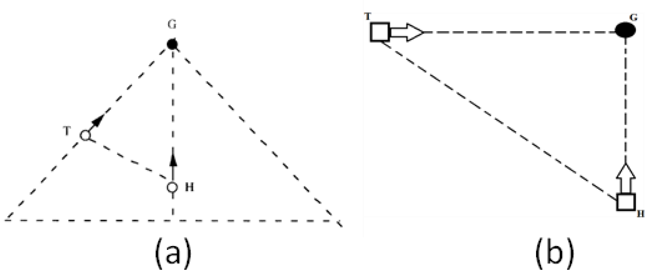
1.1. Tau-Coupling
1.2. Resonance
2. Materials and Methods
2.1. Participants
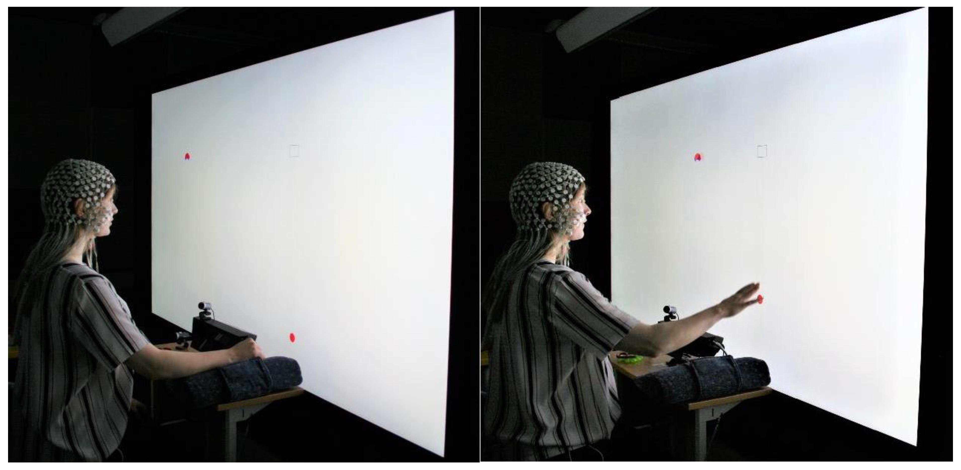
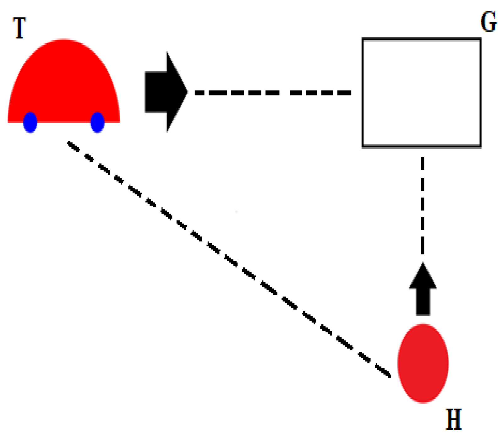
2.2. Experimental Stimuli and Paradigm
2.3. Brain Data Acquisition
2.4. Procedure
2.5. Behavioral Data Acquisition and Analyses
2.6. Brain Data Analyses and Artefact Removal
2.7. VEP and MRP Peak Analysis, and Tau-Coupling
3. Results
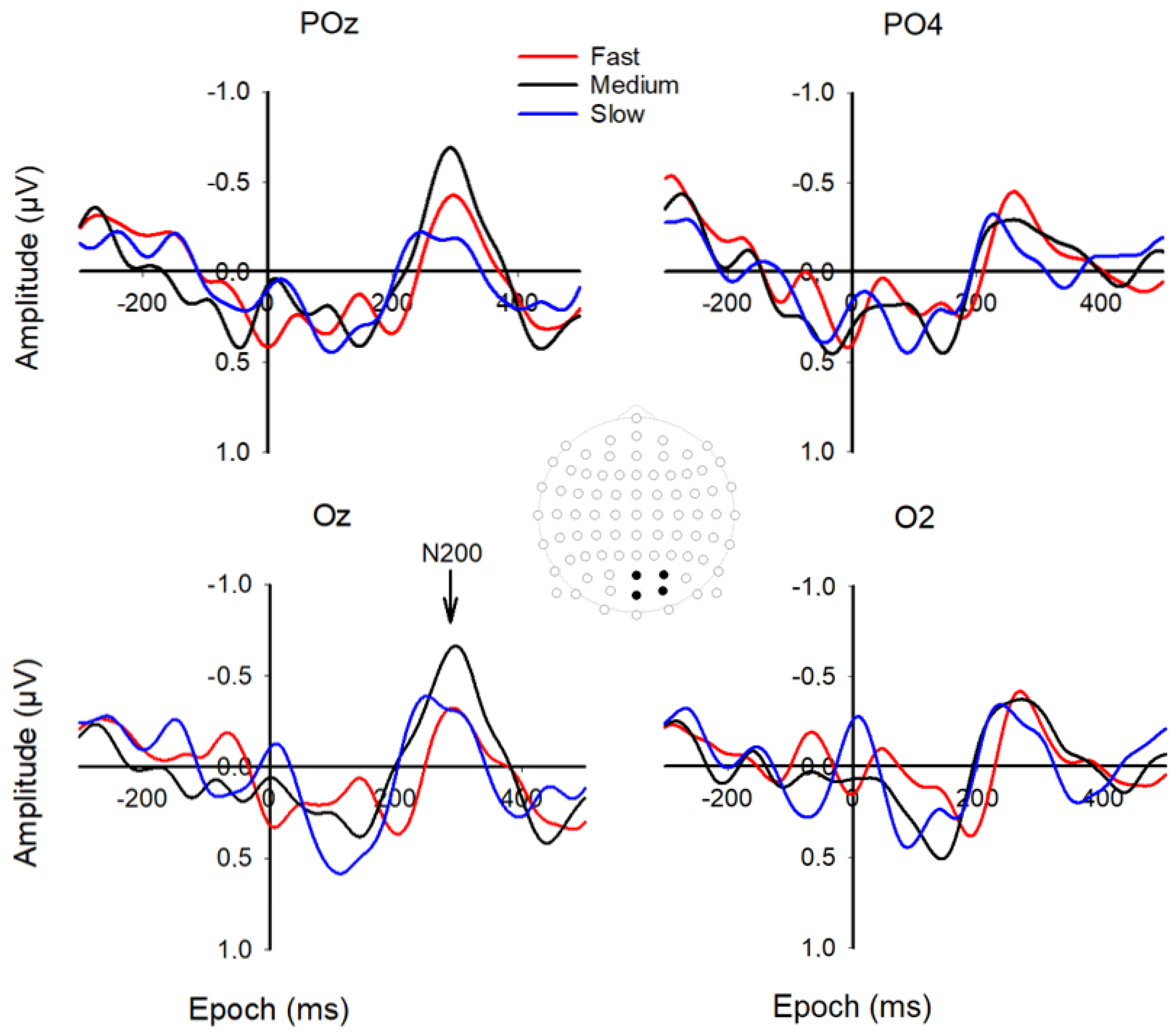
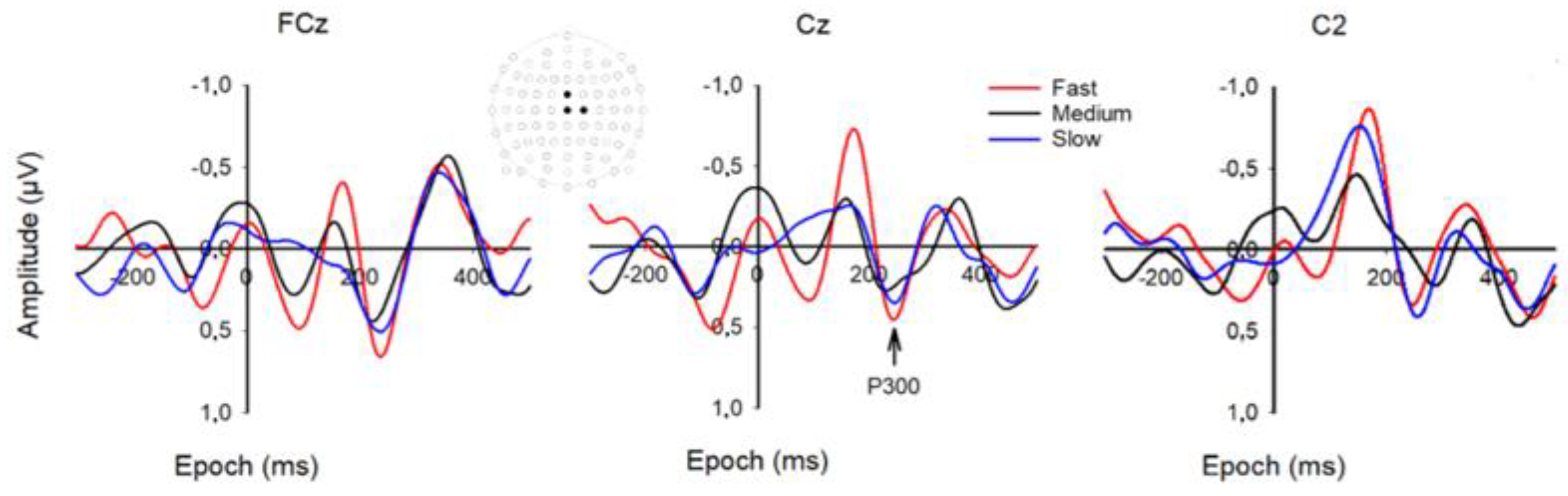
3.1. VEP and MRP Responses
3.2. Tau-Coupling Results
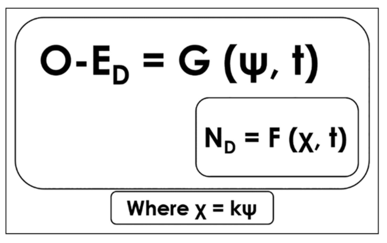
- 1. Car vs. Time
- 2. Car vs. Finger: Ecological One-Scale Indirect Comparison with Neural Scale Via k
- 3. VC (VEP) vs. MC (MRP): Neural, Same-Scale Indirect Coupling with Ecological Scale via k
- 4. VC (VEP) vs. Car: Ecological and Neural, Two-Scale Direct Comparison via kres
- 5. MC (MRP) vs. Finger: Neural and Ecological, Two-Scale Direct Comparison via kres
4. Discussion
4.1. Car vs. Time
4.2. Indirect Same-Scale τ-Coupling Analysis via k
4.2.1. At the Ecological Scale: Car vs. Finger
4.2.2. At the Neural Scale: VC (VEP) vs. MC (MRP)
4.3. Direct Two-Scale τ-Coupling Analysis via kres
4.3.1. VC (VEP) vs. Car
4.3.2. MC (MRP) vs. Finger
5. Conclusions
Supplementary Materials
Author Contributions
Funding
Institutional Review Board Statement
Informed Consent Statement
Data Availability Statement
Acknowledgments
Conflicts of Interest
References
- Lee, D.N.; Georgopoulos, A.P.; Clark, M.J.O.; Craig, C.M.; Port, N.L. Guiding contact by coupling the taus of gaps. Exp. Brain Res. 2001, 139, 151–159. [Google Scholar] [CrossRef] [PubMed]
- Alexander, R.M. A minimum energy cost hypothesis for human arm trajectories. Biol. Cybern. 1997, 76, 97–105. [Google Scholar] [CrossRef] [PubMed]
- Bizzi, E.; Mussa-Ivaldi, F.A.; Giszter, S. Does the nervous system use equilibrium-point control to guide single and multiple joint movements? Behav. Brain Sci. 1992, 15, 603–613. [Google Scholar] [CrossRef] [PubMed]
- Flash, T.; Hogan, N. The coordination of arm movements: An experimentally confirmed mathematical model. J. Neurosci. 1985, 5, 1688–1703. [Google Scholar] [CrossRef] [PubMed]
- Jeannerod, M. The Neural and Behavioral Organization of Goal-Directed Movements; Clarendon Press: Oxford, UK, 1978. [Google Scholar]
- Kelso, J.A.S. Dynamic Patterns: The Self-Organization of Brain and Behavior; MIT Press: Cambridge, MA, USA, 1995. [Google Scholar]
- Schmidt, R.C.; Turvey, M.T. Phase-entrainment dynamics of visually coupled rhythmic movements. Biol. Cybern. 1994, 70, 369–376. [Google Scholar] [CrossRef] [PubMed]
- Bootsma, R.J.; Van Wieringen, P.W.C. Timing an attacking forehand drive in table tennis. J. Exp. Psychol. Hum. Percept. Perform. 1990, 16, 21–29. [Google Scholar] [CrossRef]
- Laurent, M.; Montagne, G.; Savelsbergh, G.J.P. The control and coordination of one-handed catching: The effect of temporal constraints. Exp. Brain Res. 1994, 101, 314–322. [Google Scholar] [CrossRef]
- Port, N.L.; Lee, D.; Dassonville, P.; Georgopoulos, A.P. Manual interception of moving targets I. Performance and movement initiation. Exp. Brain Res. 1997, 116, 406–420. [Google Scholar] [CrossRef]
- Van der Meer, A.L.H.; Van der Weel, F.R.; Lee, D.N. Prospective control in catching by infants. Perception 1994, 23, 287–302. [Google Scholar] [CrossRef]
- Dienes, Z.; McLeod, P. How to catch a cricket ball. Perception 1993, 22, 1427–1439. [Google Scholar] [CrossRef]
- Georgopoulos, A.P.; Kalaska, J.F.; Massey, J.T. Spatial trajectories and reaction times of aimed movements. J. Neurophysiol. 1981, 46, 725–743. [Google Scholar] [CrossRef] [PubMed] [Green Version]
- Lee, D.N.; Davies, M.N.O.; Green, P.R.; Van der Weel, F.R. Visual control of velocity of approach by pigeons when landing. J. Exp. Biol. 1993, 180, 85–104. [Google Scholar] [CrossRef]
- Lee, D.N.; Simmons, J.A.; Saillant, P.A.; Bouffard, F. Steering by echolocation: A paradigm of ecological acoustics. J. Comp. Physiol. A 1995, 176, 347–354. [Google Scholar] [CrossRef] [PubMed]
- Lee, D.N. General Tau theory: Evolution to date. Perception 2009, 38, 837–850. [Google Scholar] [CrossRef]
- McBeath, M.K.; Schaffer, D.M.; Kaiser, M.K. How baseball outfielders determine where to run to catch fly balls. Science 1995, 268, 569–573. [Google Scholar] [CrossRef]
- Milner, T.E.; Ijaz, M.M. The effect of accuracy constraints on three-dimensional movement kinematics. Neuroscience 1990, 35, 365–374. [Google Scholar] [CrossRef]
- Oudejans, R.R.D.; Michaels, C.F.; Davids, K.; Bakker, F.C. Shedding some light on catching in the dark: Perceptual mechanisms for catching fly balls. J. Exp. Psychol. Hum. Percept. Perform. 1999, 25, 531–542. [Google Scholar] [CrossRef]
- Peper, L.; Bootsma, R.J.; Mestre, D.R.; Bakker, F.C. Catching balls: How to get the hand to the right place at the right time. J. Exp. Psychol. Hum. Percept. Perform. 1994, 20, 591–612. [Google Scholar] [CrossRef]
- Zaal, F.T.J.M.; Bootsma, R.J.; Van Wieringen, P.C.W. Coordination in prehension: Information-based coupling of reaching and grasping. Exp. Brain Res. 1998, 119, 427–435. [Google Scholar] [CrossRef] [Green Version]
- Lee, D.N. A theory of visual control of braking based on information about time-to-collision. Perception 1976, 5, 437–459. [Google Scholar] [CrossRef]
- Lee, D.N. Guiding movements by coupling taus. Ecol. Psychol. 1998, 10, 221–250. [Google Scholar] [CrossRef] [PubMed]
- Lee, D.N.; Georgopoulos, A.P.; Pepping, G.J. Prospective control of movement in the basal ganglia. bioRxiv 2018, 2, 256347. [Google Scholar] [CrossRef] [Green Version]
- Tan, H.R.; Leuthold, A.C.; Lee, D.N.; Lynch, J.K.; Georgopoulos, A.P. Neural mechanisms of movement speed and tau as revealed by magnetoencephalography. Exp. Brain Res. 2009, 195, 541–552. [Google Scholar] [CrossRef] [PubMed]
- Raja, V. From metaphor to theory: The role of resonance in perceptual learning. Adapt. Beh. 2019, 27, 405–421. [Google Scholar] [CrossRef]
- Raja, V. Resonance and radical embodiment. Synthese 2021, 199, 113–141. [Google Scholar] [CrossRef]
- Kasevich, R.S.; LaBerge, D. Theory of electric resonance in the neocortical apical dendrite. PLoS ONE 2011, 6, 1–13. [Google Scholar] [CrossRef]
- Lau, T.; Zochowsky, M. The resonance frequency shift, pattern formation, and dynamical network reorganization via sub-threshold input. PLoS ONE 2011, 6, 1–8. [Google Scholar] [CrossRef] [Green Version]
- Roach, J.P.; Pidde, A.; Katz, E.; Wu, J.; Ognjanovski, N.; Aton, S.J.; Zochowski, M.R. Resonance with subthreshold oscillatory drive organized activity and optimizes learning in neural networks. Proc. Natl. Acad. Sci. USA 2018, 115, E3017–E3025. [Google Scholar] [CrossRef] [Green Version]
- Shtrahman, E.; Zochowski, M. Pattern segmentation with activity dependent natural frequency shift and sub-threshold resonance. Sci. Rep. 2015, 5, 1–10. [Google Scholar] [CrossRef] [Green Version]
- Leonetti, A.; Puglisi, G.; Siugzdaite, R.; Ferrari, C.; Cerri, G.; Borroni, P. What you see is what you get: Motor resonance in peripheral vision. Exp. Brain Res. 2015, 233, 3013–3022. [Google Scholar] [CrossRef]
- Ikemoto, S.; DallaLibera, F.; Hosoda, K. Noise-modulated neural networks as an application of stochastic resonance. Neurocomputing 2018, 277, 29–37. [Google Scholar] [CrossRef]
- Yu, H.; Zhang, L.; Guo, X.; Wang, J.; Cao, Y.; Liu, J. Effect of inhibitory firing pattern on coherence resonance in random neural networks. Phys. A 2018, 490, 1201–1210. [Google Scholar] [CrossRef]
- Helfrich, R.; Breska, A.; Knight, R.T. Neural entrainment and network resonance in support of top-down guided attention. Curr. Opin. Psychol. 2019, 29, 82–89. [Google Scholar] [CrossRef] [PubMed]
- Grossberg, S. Adaptive resonance theory: How a brain learns to consciously attend, learn, and recognize a changing world. Neural Netw. 2013, 37, 1–47. [Google Scholar] [CrossRef]
- Grossberg, S. Conscious Mind, Resonant Brain; Oxford University Press: Oxford, UK, 2021. [Google Scholar]
- Lomas, J.D.; Lin, A.; Dikker, S.; Forster, D.; Lupetti, M.L.; Huisman, G.; Habekost, J.; Beardow, C.; Pandey, P.; Ahmad, N.; et al. Resonance as a design strategy for AI and social robots. Front. Neurorobot. 2022, 16, 850489. [Google Scholar] [CrossRef]
- Gibson, J.J. The Senses Considered as Perceptual Systems; Houghton Mifflin: Boston, MA, USA, 1966. [Google Scholar]
- Gibson, J.J. The Ecological Approach to Visual Perception; LEA: Hillsdale, NJ, USA, 1979. [Google Scholar]
- Raja, V. A theory of resonance: Towards an ecological cognitive architecture. Minds Mach. 2018, 28, 29–51. [Google Scholar] [CrossRef]
- Van der Weel, F.R.; Van der Meer, A.L.H. Seeing it coming: Infants’ brain responses to looming danger. Naturwissenschaften 2009, 96, 1385–1391. [Google Scholar] [CrossRef] [PubMed]
- Raja, V.; Anderson, M.L. Radical embodied cognitive neuroscience. Ecol. Psychol. 2019, 31, 166–181. [Google Scholar] [CrossRef]
- Tucker, D.M. Spatial sampling of head electrical fields: The geodesic sensor net. Electroencephalogr. Clin. Neurophysiol. 1993, 87, 154–163. [Google Scholar] [CrossRef]
- Picton, T.W.; Bentin, S.; Berg, P.; Donchin, E.; Hillyard, S.A.; Johnson, R.J.; Miller, G.A.; Ritter, W.; Ruchkin, D.S.; Rugg, M.D.; et al. Guidelines for using human event-related potentials to study cognition: Recording standards and publication criteria. Psychophysiology 2000, 37, 127–152. [Google Scholar] [CrossRef]
- Bosco, G.; Carrozzo, M.; Lacquaniti, F. Contributions of the human temporoparietal junction and MT/V5+ to the timing of interception revealed by transcranial magnetic stimulation. J. Neurosci. 2008, 28, 12071–12084. [Google Scholar] [CrossRef] [PubMed] [Green Version]
- Delle Monache, S.; Lacquaniti, F.; Gianfranco, B. Differential contributions to the interception of occluded ballistic trajectories by the temporoparietal junction, area hMT/V5+, and the intraparietal cortex. J. Neurophysiol. 2017, 118, 1809–1823. [Google Scholar] [CrossRef] [PubMed] [Green Version]
- Schenk, T.; Ellison, A.; Rice, N.; Milner, A. The role of V5/MT+ in the control of catching movements: An rTMS study. Neuropsychologia 2005, 43, 189–198. [Google Scholar] [CrossRef] [PubMed] [Green Version]
- Battaglia-Mayer, A.; Buiatti, T.; Caminiti, R.; Ferraina, S.; Lacquaniti, F.; Shallice, T. Correction and suppression of reaching movements in the cerebral cortex: Physiological and Neuropsychological aspects. Neurosci. Biobehav. Rev. 2014, 42, 232–251. [Google Scholar] [CrossRef] [Green Version]
- Caminiti, R.; Fet-Rainat, S.; Battaglia-Mayer, A. Visuomotor transformations: Early cortical mechanisms of reaching. Curr. Opin. Neurobiol. 1998, 8, 753–761. [Google Scholar] [CrossRef]
- Dessing, J.; Vesia, M.; Crawford, J. The role of areas MT+/V5 and SPOC in spatial and temporal control of manual interception: An rTMS study. Front. Behav. Neurosci. 2013, 7, 1–15. [Google Scholar] [CrossRef] [Green Version]
- Lee, D.; Port, N.L.; Kruse, W.; Georgopoulos, A.P. Neuronal clusters in the primate motor cortex during interception of moving targets. J. Cogn. Neurosci. 2001, 13, 319–331. [Google Scholar] [CrossRef]
- Merchant, H.; Georgopoulos, A.P. Neurophysiology of perceptual and motor aspects of interception. J. Neurophysiol. 2006, 95, 1–13. [Google Scholar] [CrossRef]
- Port, N.L.; Kruse, W.; Lee, D.; Georgopoulos, A.P. Motor cortical activity during interception of moving targets. J. Cogn. Neurosci. 2001, 13, 306–318. [Google Scholar] [CrossRef]
- Merchant, H.; Battaglia-Mayer, A.; Georgopoulos, A.P. Neural responses during interception of real and apparent circularly moving stimuli in motor cortex and area 7a. Cereb. Cortex 2004, 14, 314–331. [Google Scholar] [CrossRef]
- Pitzalis, S.; Strappini, F.; De Gasperis, M.; Bltrini, A.; Di Russo, F. Spatio-temporal brain mapping of motion-onset VEPs combined with fMRI and retinotopic maps. PLoS ONE 2013, 7, 1–13. [Google Scholar] [CrossRef] [PubMed] [Green Version]
- Probst, T.; Plendl, H.; Paulus, W.; Wist, E.; Scherg, M. Experimental brain research identification of the visual motion area (area V5) in the human brain by dipole source analysis. Exp. Brain Res. 1993, 93, 3704–3709. [Google Scholar] [CrossRef] [PubMed]
- Vilhelmsen, K.; Agyei, S.B.; Van der Weel, F.R.; Van der Meer, A.L.H. A high-density EEG study of differentiation between two speeds and directions of simulated optic flow in adults and infants. Psychophysiology 2019, 56, 1–15. [Google Scholar] [CrossRef] [PubMed]
- Vilhelmsen, K.; Van der Weel, F.R.; Van der Meer, A.L.H. A high-density EEG study of differences between three high speeds of simulated forward motion from optic flow in adult participants. Front. Syst. Neurosci. 2015, 9, 1–10. [Google Scholar] [CrossRef] [Green Version]
- Berndt, I.; Franz, V.; Bülthoff, H.; Wascher, E. Effects of pointing direction and direction predictability on event-related lateralizations of the EEG. Hum. Mov. Sci. 2002, 21, 387–410. [Google Scholar] [CrossRef]
- Bozzacchi, C.; Giusti, M.; Pitzalis, S.; Spinelli, D.; Di Russo, F. Awareness affects motor planning for goal-directed actions. Biol. Psych. 2012, 89, 503–514. [Google Scholar] [CrossRef]
- McDowell, K.; Jeka, J.; Schöner, G.; Hatfield, B. Behavioral and electrocortical evidence of an interaction between probability and task metrics in movement preparation. Exp. Brain Res. 2002, 144, 303–313. [Google Scholar] [CrossRef]
- Naranjo, J.; Brovelli, A.; Longo, R.; Budai, R.; Kristeva, R.; Battaglini, P. EEG dynamics of the frontoparietal network during reaching preparation in humans. NeuroImage 2007, 34, 1673–1682. [Google Scholar] [CrossRef]
- Tarantino, V.; De Sanctis, T.; Straulino, E.; Begliomini, C.; Castiello, U. Object size modulates fronto-parietal activity during reaching movements. Eur. J. Neurosci. 2014, 39, 1528–1537. [Google Scholar] [CrossRef]
- Folstein, J.R.; Van Petten, C. Influence of cognitive control and mismatch on the N2 component of the ERP: A review. Psychophysiology 2008, 45, 152–170. [Google Scholar] [CrossRef]
- Polich, J. Updating P300: An integrative theory of P3a and P3b. Clin. Neurophysiol. 2007, 118, 2128–2148. [Google Scholar] [CrossRef] [PubMed] [Green Version]
- Van der Weel, F.R.; Agyei, S.B.; Van der Meer, A.L.H. Infants’ brain responses to looming danger: Degeneracy of neural connectivity patterns. Ecol. Psychol. 2019, 31, 182–197. [Google Scholar] [CrossRef]
- Segundo-Ortín, M.; Heras-Escribano, M.; Raja, V. Ecological psychology is radical enough: A reply to radical enactivists. Philos. Psychol. 2019, 32, 1001–1023. [Google Scholar] [CrossRef] [Green Version]
- Warren, W.H. Information is where you find it: Perception as an ecologically well-posed problem. i-Perception 2021, 12, 1–24. [Google Scholar] [CrossRef] [PubMed]
- Kayed, N.S.; Van der Meer, A.L.H. A longitudinal study of prospective control in catching by full-term and preterm infants. Exp. Brain Res. 2009, 194, 245–258. [Google Scholar] [CrossRef]
- Mueller, A.S.; Timney, B. Visual acceleration perception for simple and complex motion patterns. PLoS ONE 2016, 11, 1–10. [Google Scholar] [CrossRef]
- Aguilera, M.; Bedia, M.G.; Santos, B.A.; Barandiaran, X.E. The situated HKB model: How sensorimotor spatial coupling can alter oscillatory brain dynamics. Front. Comp. Neurosci. 2013, 7, 117. [Google Scholar] [CrossRef] [Green Version]
- Kelso, J.A.S.; Tognoli, E. Toward a complementary neuroscience: Metastable coordination dynamics of the brain. In Neurodynamics of Cognition and Consciousness; Perlovsky, L.I., Kozma, R., Eds.; Springer: Berlin/Heidelberg, Germany, 2007; pp. 39–59. [Google Scholar]
- Large, E.W. Resonating to musical rhythm: Theory and experiment. In The Psychology of Time; Grondin, S., Ed.; Emerald: West Yorkshire, UK, 2008. [Google Scholar]
- Safont, G.; Salazar, A.; Vergara, L.; Gómez, E.; Villanueva, V. Multichannel dynamic modeling of non-Gaussian mixtures. Pattern Recognit. 2019, 93, 312–323. [Google Scholar] [CrossRef]
- De Wit, M.M.; Withagen, R. What should a “Gibsonian Neuroscience” look like? Introduction to the special issue. Ecol. Psychol. 2019, 31, 147–151. [Google Scholar] [CrossRef]


| Type of τ-Coupling | Resonance Scale | Slow (SD) | Medium (SD) | Fast (SD) |
|---|---|---|---|---|
| 1. Car vs. Time (benchmark values) | Ecological scale (not a τ-coupling as such) | 0.88 (0.06) | 0.99 (0.09) | 1.12 (0.09) |
| 2. Car vs. Finger | Ecological, same-scale indirect coupling comparison with neural scale via k | 0.99 (0.07) | 1.11 (0.09) | 1.26 (0.08) |
| 3. VC (VEP) vs. MC (MRP) | Neural, same-scale indirect coupling comparison with ecological scale via k | 0.98 (0.14) | 1.06 (0.16) | 1.27 (0.17) |
| 4. VC (VEP) vs. Car | Ecological and neural, two-scale direct coupling comparison via kres | 0.81 (0.09) | 0.90 (0.13) | 1.03 (0.13) |
| 5. MC (MRP) vs. Finger | Neural and ecological, two-scale direct comparison via kres | 0.80 (0.15) | 1.02 (0.32) | 1.36 (0.39) * |
Publisher’s Note: MDPI stays neutral with regard to jurisdictional claims in published maps and institutional affiliations. |
© 2022 by the authors. Licensee MDPI, Basel, Switzerland. This article is an open access article distributed under the terms and conditions of the Creative Commons Attribution (CC BY) license (https://creativecommons.org/licenses/by/4.0/).
Share and Cite
van der Weel, F.R.; Sokolovskis, I.; Raja, V.; van der Meer, A.L.H. Neural Aspects of Prospective Control through Resonating Taus in an Interceptive Timing Task. Brain Sci. 2022, 12, 1737. https://doi.org/10.3390/brainsci12121737
van der Weel FR, Sokolovskis I, Raja V, van der Meer ALH. Neural Aspects of Prospective Control through Resonating Taus in an Interceptive Timing Task. Brain Sciences. 2022; 12(12):1737. https://doi.org/10.3390/brainsci12121737
Chicago/Turabian Stylevan der Weel, F. R. (Ruud), Ingemārs Sokolovskis, Vicente Raja, and Audrey L. H. van der Meer. 2022. "Neural Aspects of Prospective Control through Resonating Taus in an Interceptive Timing Task" Brain Sciences 12, no. 12: 1737. https://doi.org/10.3390/brainsci12121737
APA Stylevan der Weel, F. R., Sokolovskis, I., Raja, V., & van der Meer, A. L. H. (2022). Neural Aspects of Prospective Control through Resonating Taus in an Interceptive Timing Task. Brain Sciences, 12(12), 1737. https://doi.org/10.3390/brainsci12121737