
Bayesian Optimization of Machine Learning Classification of Resting-State EEG Microstates in Schizophrenia: A Proof-of-Concept Preliminary Study Based on Secondary Analysis

Abstract
1. Introduction
2. Materials and Methods
2.1. Dataset
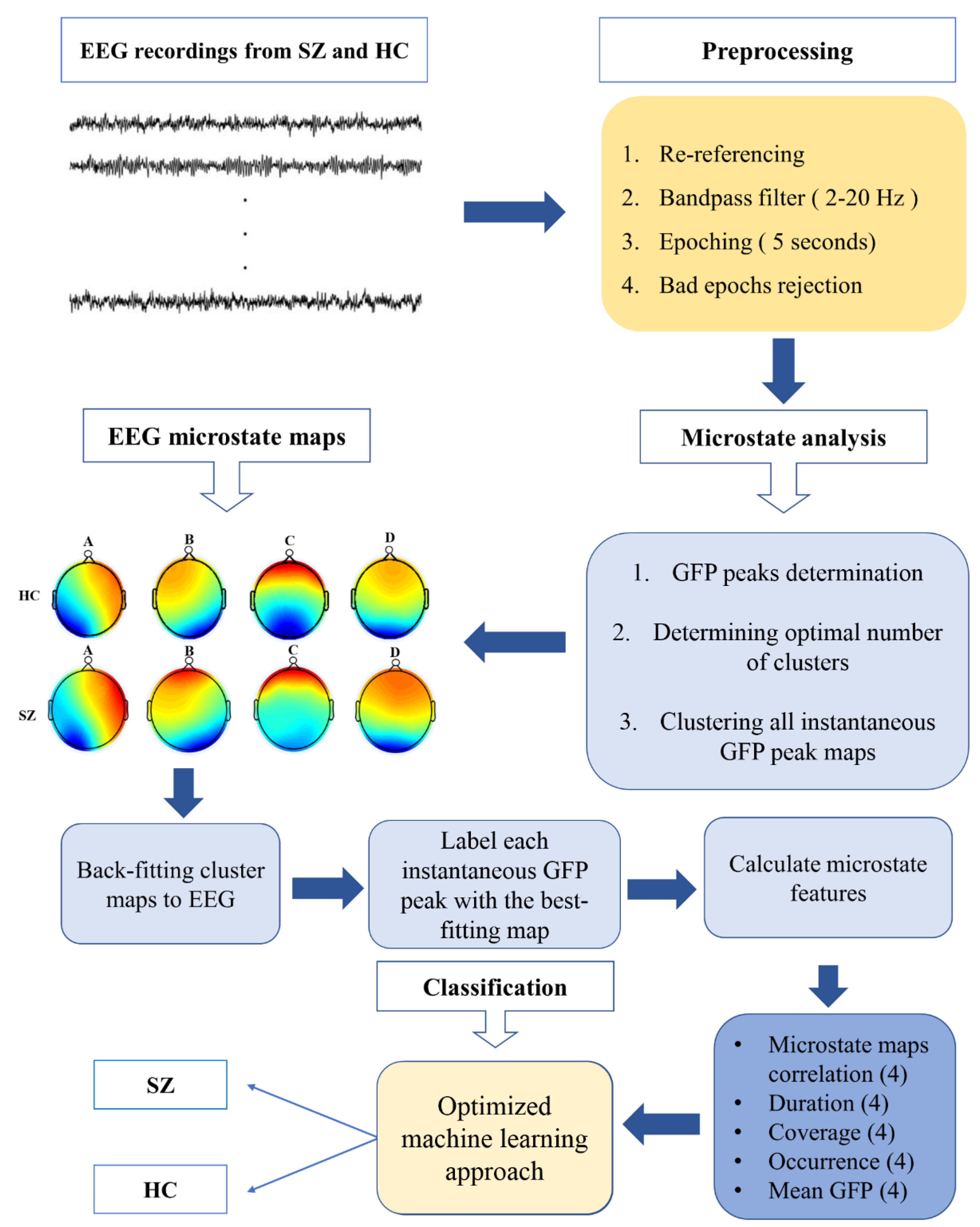
2.2. EEG Data Pre-Processing
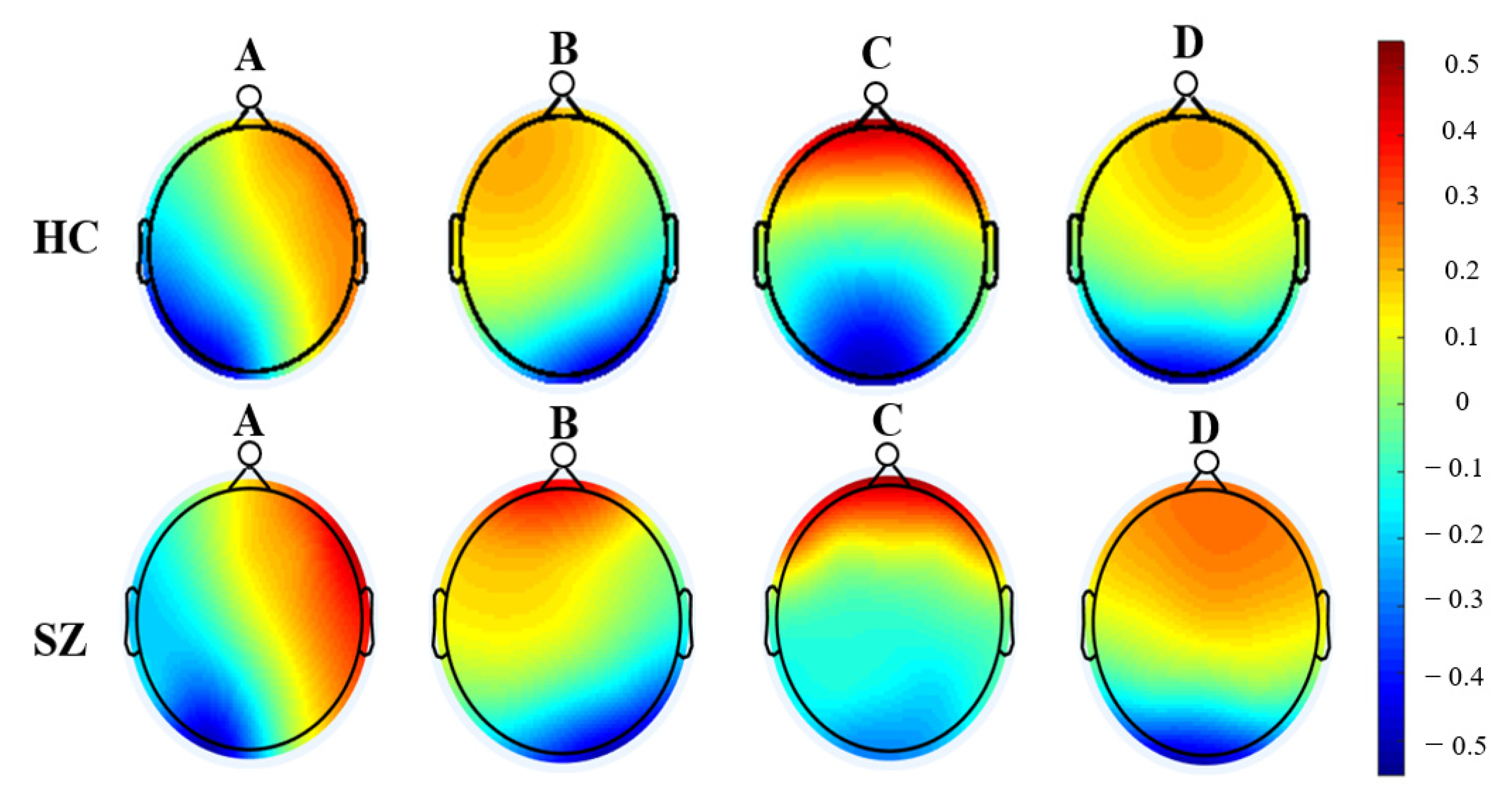
2.3. Microstate Analysis
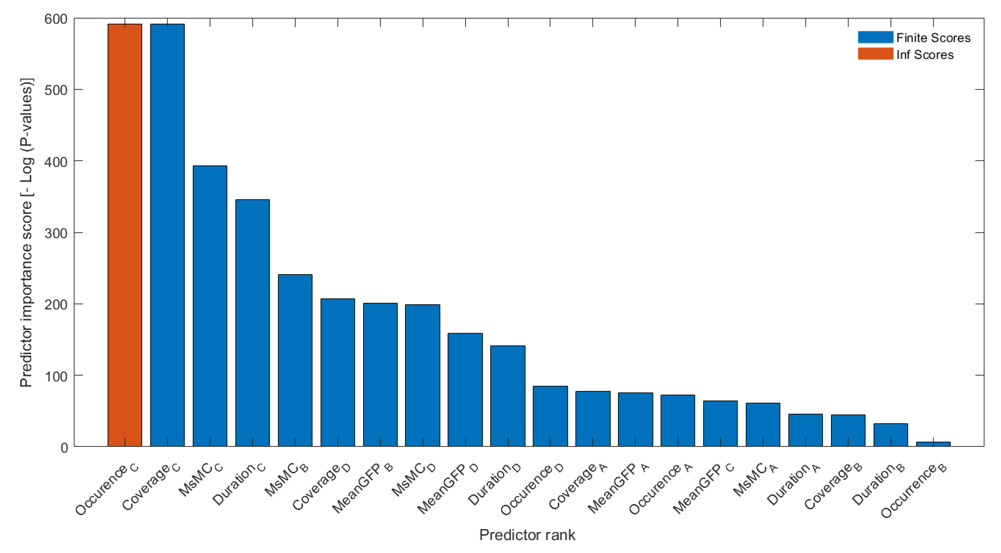
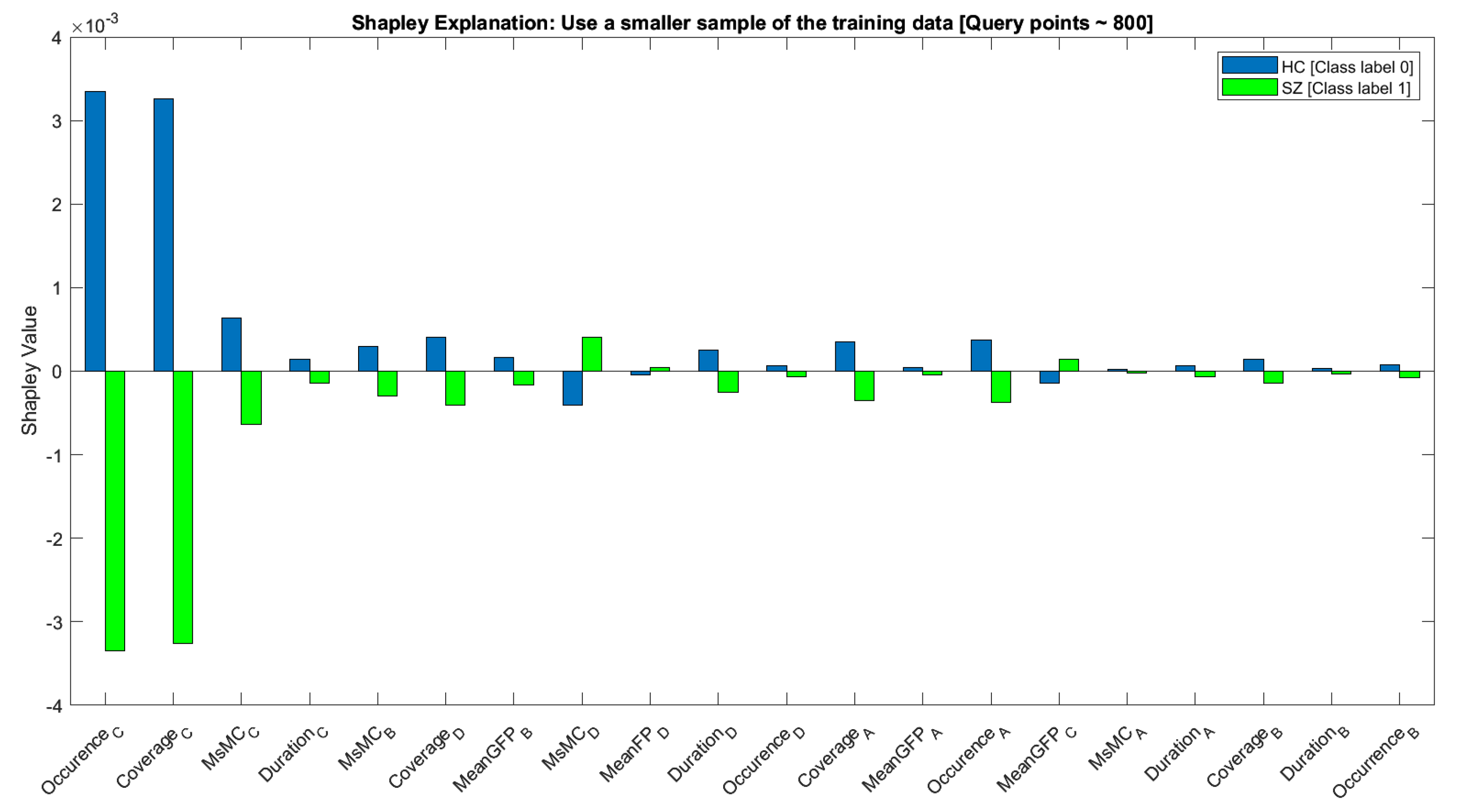
2.4. Predictors’ Ranking and Classification
2.5. Bayesian Optimization of Classification
3. Results
4. Discussion
5. Conclusions
Supplementary Materials
Author Contributions
Funding
Institutional Review Board Statement
Informed Consent Statement
Data Availability Statement
Acknowledgments
Conflicts of Interest
References
- Bleuler, E. Dementia Praecox or the Group of Schizophrenias; International Universities Press: New York, NY, USA, 1950. [Google Scholar]
- Kraepelin, E. Dementia Praecox and Paraphrenia; Barclay, R.M., Translator; Krieger: Huntingdon, NY, USA, 1919. [Google Scholar]
- Vignapiano, A.; Koenig, T.; Mucci, A.; Giordano, G.M.; Amodio, A.; Altamura, M.; Bellomo, A.; Brugnoli, R.; Corrivetti, G.; Di Lorenzo, G. Disorganization and cognitive impairment in schizophrenia: New insights from electrophysiological findings. Int. J. Psychophysiol. 2019, 145, 99–108. [Google Scholar] [CrossRef] [PubMed]
- McCleery, A.; Lee, J.; Joshi, A.; Wynn, J.K.; Hellemann, G.S.; Green, M.F. Meta-analysis of face processing event-related potentials in schizophrenia. Biol. Psychiatry 2015, 77, 116–126. [Google Scholar] [CrossRef] [PubMed]
- Haigh, S.M.; Coffman, B.A.; Salisbury, D.F. Mismatch negativity in first-episode schizophrenia: A meta-analysis. Clin. EEG Neurosci. 2017, 48, 3–10. [Google Scholar] [CrossRef] [PubMed]
- Ferrarelli, F. Sleep abnormalities in schizophrenia: State of the art and next steps. Am. J. Psychiatry 2021, 178, 903–913. [Google Scholar] [CrossRef] [PubMed]
- Chan, M.-S.; Chung, K.-F.; Yung, K.-P.; Yeung, W.-F. Sleep in schizophrenia: A systematic review and meta-analysis of polysomnographic findings in case-control studies. Sleep Med. Rev. 2017, 32, 69–84. [Google Scholar] [CrossRef] [PubMed]
- Kambeitz, J.; Kambeitz-Ilankovic, L.; Cabral, C.; Dwyer, D.B.; Calhoun, V.D.; Van Den Heuvel, M.P.; Falkai, P.; Koutsouleris, N.; Malchow, B. Aberrant functional whole-brain network architecture in patients with schizophrenia: A meta-analysis. Schizophr. Bull. 2016, 42, S13–S21. [Google Scholar] [CrossRef] [PubMed]
- Craig, N.; Coppola, R.; Morihisa, J.M.; Weinberger, D.R. Computed electroencephalographic activity mapping in schizophrenia: The resting state reconsidered. Arch. Gen. Psychiatry 1987, 44, 514–517. [Google Scholar]
- Kam, J.W.; Bolbecker, A.R.; O’Donnell, B.F.; Hetrick, W.P.; Brenner, C.A. Resting state EEG power and coherence abnormalities in bipolar disorder and schizophrenia. J. Psychiatr. Res. 2013, 47, 1893–1901. [Google Scholar] [CrossRef]
- Sueyoshi, K.; Sumiyoshi, T. Electrophysiological evidence in schizophrenia in relation to treatment response. Front. Psychiatry 2018, 9, 259. [Google Scholar] [CrossRef]
- Alimardani, F.; Cho, J.-H.; Boostani, R.; Hwang, H.-J. Classification of bipolar disorder and schizophrenia using steady-state visual evoked potential based features. IEEE Access 2018, 6, 40379–40388. [Google Scholar] [CrossRef]
- Tikka, S.K.; Singh, B.K.; Nizamie, S.H.; Garg, S.; Mandal, S.; Thakur, K.; Singh, L.K. Artificial intelligence-based classification of schizophrenia: A high density electroencephalographic and support vector machine study. Indian J. Psychiatry 2020, 62, 273. [Google Scholar] [CrossRef] [PubMed]
- Koenig, T.; Lehmann, D.; Merlo, M.C.; Kochi, K.; Hell, D.; Koukkou, M. A deviant EEG brain microstate in acute, neuroleptic-naive schizophrenics at rest. Eur. Arch. Psychiatry Clin. Neurosci. 1999, 249, 205–211. [Google Scholar] [CrossRef] [PubMed]
- Lehmann, D.; Faber, P.L.; Galderisi, S.; Herrmann, W.M.; Kinoshita, T.; Koukkou, M.; Mucci, A.; Pascual-Marqui, R.D.; Saito, N.; Wackermann, J. EEG microstate duration and syntax in acute, medication-naive, first-episode schizophrenia: A multi-center study. Psychiatry Res. Neuroimaging 2005, 138, 141–156. [Google Scholar] [CrossRef] [PubMed]
- Strelets, V.; Faber, P.; Golikova, J.; Novototsky-Vlasov, V.; König, T.; Gianotti, L.; Gruzelier, J.; Lehmann, D. Chronic schizophrenics with positive symptomatology have shortened EEG microstate durations. Clin. Neurophysiol. 2003, 114, 2043–2051. [Google Scholar] [CrossRef]
- Tomescu, M.I.; Rihs, T.A.; Roinishvili, M.; Karahanoglu, F.I.; Schneider, M.; Menghetti, S.; Van De Ville, D.; Brand, A.; Chkonia, E.; Eliez, S. Schizophrenia patients and 22q11. 2 deletion syndrome adolescents at risk express the same deviant patterns of resting state EEG microstates: A candidate endophenotype of schizophrenia. Schizophr. Res. Cogn. 2015, 2, 159–165. [Google Scholar] [CrossRef]
- Rieger, K.; Diaz Hernandez, L.; Baenninger, A.; Koenig, T. 15 years of microstate research in schizophrenia–where are we? A meta-analysis. Front. Psychiatry 2016, 7, 22. [Google Scholar] [CrossRef]
- Lehmann, D.; Ozaki, H.; Pál, I. EEG alpha map series: Brain micro-states by space-oriented adaptive segmentation. Electroencephalogr. Clin. Neurophysiol. 1987, 67, 271–288. [Google Scholar] [CrossRef]
- Seitzman, B.A.; Abell, M.; Bartley, S.C.; Erickson, M.A.; Bolbecker, A.R.; Hetrick, W.P. Cognitive manipulation of brain electric microstates. Neuroimage 2017, 146, 533–543. [Google Scholar] [CrossRef]
- Lehmann, D.; Strik, W.K.; Henggeler, B.; König, T.; Koukkou, M. Brain electric microstates and momentary conscious mind states as building blocks of spontaneous thinking: I. Visual imagery and abstract thoughts. Int. J. Psychophysiol. 1998, 29, 1–11. [Google Scholar] [CrossRef]
- Britz, J.; Van De Ville, D.; Michel, C.M. BOLD correlates of EEG topography reveal rapid resting-state network dynamics. Neuroimage 2010, 52, 1162–1170. [Google Scholar] [CrossRef]
- Zappasodi, F.; Perrucci, M.G.; Saggino, A.; Croce, P.; Mercuri, P.; Romanelli, R.; Colom, R.; Ebisch, S.J. EEG microstates distinguish between cognitive components of fluid reasoning. Neuroimage 2019, 189, 560–573. [Google Scholar] [CrossRef] [PubMed]
- Bowers, K.S. Imagination and dissociation in hypnotic responding. Int. J. Clin. Exp. Hypn. 1992, 40, 253–275. [Google Scholar] [CrossRef] [PubMed]
- Milz, P.; Faber, P.L.; Lehmann, D.; Koenig, T.; Kochi, K.; Pascual-Marqui, R.D. The functional significance of EEG microstates—Associations with modalities of thinking. Neuroimage 2016, 125, 643–656. [Google Scholar] [CrossRef]
- Yuan, H.; Zotev, V.; Phillips, R.; Drevets, W.C.; Bodurka, J. Spatiotemporal dynamics of the brain at rest—Exploring EEG microstates as electrophysiological signatures of BOLD resting state networks. Neuroimage 2012, 60, 2062–2072. [Google Scholar] [CrossRef] [PubMed]
- Kim, K.; Duc, N.T.; Choi, M.; Lee, B. EEG microstate features for schizophrenia classification. PLoS ONE 2021, 16, e0251842. [Google Scholar] [CrossRef] [PubMed]
- Lehmann, D.; Pascual-Marqui, R.; Michel, C. EEG microstates. Scholarpedia 2009, 4, 7632. [Google Scholar] [CrossRef]
- Mackintosh, A.J.; Borgwardt, S.; Studerus, E.; Riecher-Rössler, A.; De Bock, R.; Andreou, C. EEG microstate differences in medicated vs. Medication-Naïve first-episode psychosis patients. Front. Psychiatry 2020, 11, 600606. [Google Scholar] [CrossRef]
- Baradits, M.; Bitter, I.; Czobor, P. Multivariate patterns of EEG microstate parameters and their role in the discrimination of patients with schizophrenia from healthy controls. Psychiatry Res. 2020, 288, 112938. [Google Scholar] [CrossRef]
- Barros, C.; Silva, C.A.; Pinheiro, A.P. Advanced EEG-based learning approaches to predict schizophrenia: Promises and pitfalls. Artif. Intell. Med. 2021, 114, 102039. [Google Scholar] [CrossRef]
- Khanna, A.; Pascual-Leone, A.; Michel, C.M.; Farzan, F. Microstates in resting-state EEG: Current status and future directions. Neurosci. Biobehav. Rev. 2015, 49, 105–113. [Google Scholar] [CrossRef]
- Poulsen, A.T.; Pedroni, A.; Langer, N.; Hansen, L.K. Microstate EEGlab toolbox: An introductory guide. BioRxiv 2018, 289850. [Google Scholar] [CrossRef]
- Hu, W.; Zhang, Z.; Zhang, L.; Huang, G.; Li, L.; Liang, Z. Microstate Detection in Naturalistic Electroencephalography Data: A Systematic Comparison of Topographical Clustering Strategies on an Emotional Database. Front. Neurosci. 2022, 16, 812624. [Google Scholar] [CrossRef] [PubMed]
- Wu, J.; Chen, X.-Y.; Zhang, H.; Xiong, L.-D.; Lei, H.; Deng, S.-H. Hyperparameter optimization for machine learning models based on Bayesian optimization. J. Electron. Sci. Technol. 2019, 17, 26–40. [Google Scholar]
- Bergstra, J.; Bengio, Y. Random search for hyper-parameter optimization. J. Mach. Learn. Res. 2012, 13, 281–305. [Google Scholar]
- Gelbart, M.A.; Snoek, J.; Adams, R.P. Bayesian optimization with unknown constraints. arXiv 2014, arXiv:1403.5607. [Google Scholar]
- Snoek, J.; Larochelle, H.; Adams, R.P. Practical bayesian optimization of machine learning algorithms. Adv. Neural Inf. Process. Syst. 2012, 25. [Google Scholar] [CrossRef]
- Jones, D.R. A taxonomy of global optimization methods based on response surfaces. J. Glob. Optim. 2001, 21, 345–383. [Google Scholar] [CrossRef]
- Lillo, E.; Mora, M.; Lucero, B. Automated diagnosis of schizophrenia using EEG microstates and Deep Convolutional Neural Network. Expert Syst. Appl. 2022, 209, 118236. [Google Scholar] [CrossRef]
- Alves, L.M.; Côco, K.F.; de Souza, M.L.; Ciarelli, P.M. Microstate Graphs: A Node-Link Approach to Identify Patients with Schizophrenia. In Proceedings of the Brazilian Congress on Biomedical Engineering, Vitória, Brazil, 26–30 October 2020; pp. 1679–1685. [Google Scholar]
- Olejarczyk, E.; Jernajczyk, W. Graph-based analysis of brain connectivity in schizophrenia. PLoS ONE 2017, 12, e0188629. [Google Scholar] [CrossRef]
- Olejarczyk, E.; Jernajczyk, W. EEG in schizophrenia. RepOD 2017. [Google Scholar] [CrossRef]
- Delorme, A.; Makeig, S. EEGLAB: An open source toolbox for analysis of single-trial EEG dynamics including independent component analysis. J. Neurosci. Methods 2004, 134, 9–21. [Google Scholar] [CrossRef] [PubMed]
- Koenig, T.; Prichep, L.; Lehmann, D.; Sosa, P.V.; Braeker, E.; Kleinlogel, H.; Isenhart, R.; John, E.R. Millisecond by millisecond, year by year: Normative EEG microstates and developmental stages. Neuroimage 2002, 16, 41–48. [Google Scholar] [CrossRef] [PubMed]
- Wackermann, J.; Lehmann, D.; Michel, C.; Strik, W. Adaptive segmentation of spontaneous EEG map series into spatially defined microstates. Int. J. Psychophysiol. 1993, 14, 269–283. [Google Scholar] [CrossRef]
- Lehmann, D.; Skrandies, W. Reference-free identification of components of checkerboard-evoked multichannel potential fields. Electroencephalogr. Clin. Neurophysiol. 1980, 48, 609–621. [Google Scholar] [CrossRef]
- Michel, C.M.; Koenig, T. EEG microstates as a tool for studying the temporal dynamics of whole-brain neuronal networks: A review. Neuroimage 2018, 180, 577–593. [Google Scholar] [CrossRef]
- Murray, M.M.; Brunet, D.; Michel, C.M. Topographic ERP analyses: A step-by-step tutorial review. Brain Topogr. 2008, 20, 249–264. [Google Scholar] [CrossRef]
- Hussain, I.; Park, S.J. HealthSOS: Real-time health monitoring system for stroke prognostics. IEEE Access 2020, 8, 213574–213586. [Google Scholar] [CrossRef]
- Hussain, I.; Park, S.-J. Quantitative evaluation of task-induced neurological outcome after stroke. Brain Sci. 2021, 11, 900. [Google Scholar] [CrossRef]
- Choi, W.; Park, E.-Y.; Jeon, S.; Kim, C. Clinical photoacoustic imaging platforms. Biomed. Eng. Lett. 2018, 8, 139–155. [Google Scholar] [CrossRef]
- Tahernezhad-Javazm, F.; Azimirad, V.; Shoaran, M. A review and experimental study on the application of classifiers and evolutionary algorithms in EEG-based brain–machine interface systems. J. Neural Eng. 2018, 15, 021007. [Google Scholar] [CrossRef]
- Keihani, A.; Mohammadi, A.M.; Marzbani, H.; Nafissi, S.; Haidari, M.R.; Jafari, A.H. Sparse representation of brain signals offers effective computation of cortico-muscular coupling value to predict the task-related and non-task sEMG channels: A joint hdEEG-sEMG study. PLoS ONE 2022, 17, e0270757. [Google Scholar] [CrossRef] [PubMed]
- Hussain, I.; Park, S.J. Big-ECG: Cardiographic predictive cyber-physical system for stroke management. IEEE Access 2021, 9, 123146–123164. [Google Scholar] [CrossRef]
- Bull, A.D. Convergence rates of efficient global optimization algorithms. J. Mach. Learn. Res. 2011, 12, 2879–2904. [Google Scholar]
- Li, L.; Jamieson, K.; Rostamizadeh, A.; Gonina, E.; Ben-Tzur, J.; Hardt, M.; Recht, B.; Talwalkar, A. A system for massively parallel hyperparameter tuning. Proc. Mach. Learn. Syst. 2020, 2, 230–246. [Google Scholar]
- Noble, W.S. What is a support vector machine? Nat. Biotechnol. 2006, 24, 1565–1567. [Google Scholar] [CrossRef]
- Wang, F.; Hujjaree, K.; Wang, X. Electroencephalographic microstates in schizophrenia and bipolar disorder. Front. Psychiatry 2021, 12, 638722. [Google Scholar] [CrossRef]
- Custo, A.; Van De Ville, D.; Wells, W.M.; Tomescu, M.I.; Brunet, D.; Michel, C.M. Electroencephalographic resting-state networks: Source localization of microstates. Brain Connect. 2017, 7, 671–682. [Google Scholar] [CrossRef]
- Yang, G.J.; Murray, J.D.; Repovs, G.; Cole, M.W.; Savic, A.; Glasser, M.F.; Pittenger, C.; Krystal, J.H.; Wang, X.-J.; Pearlson, G.D. Altered global brain signal in schizophrenia. Proc. Natl. Acad. Sci. USA 2014, 111, 7438–7443. [Google Scholar] [CrossRef]
- Kowalski, J.; Aleksandrowicz, A.; Dąbkowska, M.; Gawęda, Ł. Neural Correlates of Aberrant Salience and Source Monitoring in Schizophrenia and At-Risk Mental States—A Systematic Review of fMRI Studies. J. Clin. Med. 2021, 10, 4126. [Google Scholar] [CrossRef]
- White, T.P.; Joseph, V.; Francis, S.T.; Liddle, P.F. Aberrant salience network (bilateral insula and anterior cingulate cortex) connectivity during information processing in schizophrenia. Schizophr. Res. 2010, 123, 105–115. [Google Scholar] [CrossRef]
- Palaniyappan, L.; White, T.P.; Liddle, P.F. The concept of salience network dysfunction in schizophrenia: From neuroimaging observations to therapeutic opportunities. Curr. Top. Med. Chem. 2012, 12, 2324–2338. [Google Scholar] [CrossRef] [PubMed]
- Nishida, K.; Morishima, Y.; Yoshimura, M.; Isotani, T.; Irisawa, S.; Jann, K.; Dierks, T.; Strik, W.; Kinoshita, T.; Koenig, T. EEG microstates associated with salience and frontoparietal networks in frontotemporal dementia, schizophrenia and Alzheimer’s disease. Clin. Neurophysiol. 2013, 124, 1106–1114. [Google Scholar] [CrossRef] [PubMed]
- Yoshimura, M.; Koenig, T.; Irisawa, S.; Isotani, T.; Yamada, K.; Kikuchi, M.; Okugawa, G.; Yagyu, T.; Kinoshita, T.; Strik, W. A pharmaco-EEG study on antipsychotic drugs in healthy volunteers. Psychopharmacology 2007, 191, 995–1004. [Google Scholar] [CrossRef] [PubMed]
- Fioravanti, M.; Bianchi, V.; Cinti, M.E. Cognitive deficits in schizophrenia: An updated metanalysis of the scientific evidence. BMC Psychiatry 2012, 12, 64. [Google Scholar] [CrossRef] [PubMed]
- Bagherzadeh, S.; Shahabi, M.S.; Shalbaf, A. Detection of schizophrenia using hybrid of deep learning and brain effective connectivity image from electroencephalogram signal. Comput. Biol. Med. 2022, 146, 105570. [Google Scholar] [CrossRef] [PubMed]
- Khare, S.K.; Bajaj, V.; Acharya, U.R. Spwvd-cnn for automated detection of schizophrenia patients using eeg signals. IEEE Trans. Instrum. Meas. 2021, 70, 2507409. [Google Scholar] [CrossRef]
- Oh, S.L.; Vicnesh, J.; Ciaccio, E.J.; Yuvaraj, R.; Acharya, U.R. Deep convolutional neural network model for automated diagnosis of schizophrenia using EEG signals. Appl. Sci. 2019, 9, 2870. [Google Scholar] [CrossRef]
- Phang, C.-R.; Noman, F.; Hussain, H.; Ting, C.-M.; Ombao, H. A multi-domain connectome convolutional neural network for identifying schizophrenia from EEG connectivity patterns. IEEE J. Biomed. Health Inform. 2019, 24, 1333–1343. [Google Scholar] [CrossRef]
- Shalbaf, A.; Bagherzadeh, S.; Maghsoudi, A. Transfer learning with deep convolutional neural network for automated detection of schizophrenia from EEG signals. Phys. Eng. Sci. Med. 2020, 43, 1229–1239. [Google Scholar] [CrossRef]
- Singh, K.; Singh, S.; Malhotra, J. Spectral features based convolutional neural network for accurate and prompt identification of schizophrenic patients. Proc. Inst. Mech. Eng. Part H J. Eng. Med. 2021, 235, 167–184. [Google Scholar] [CrossRef]


| Features | Definition | Number |
|---|---|---|
| Occurrence | Occurrence of a microstate per second (Hz) | 4 |
| Duration | The average duration of a microstate (ms) | 4 |
| Coverage | Percent of time occupied by a microstate (%) | 4 |
| Mean GFP | Mean of global field power (uV) | 4 |
| Microstate map correlation (MsMC) | Spatial correlation between topographies and microstates | 4 |
| Features (Occurrence) | Type A | Type B | Type C | Type D |
|---|---|---|---|---|
| Mean ± SD [HC] | 3.65 ± 1.17 | 4.26 ± 1.39 | 4.13 ± 1.28 | 4.01 ± 1.26 |
| Mean ± SD [SZ] | 4.05 ± 1.23 | 4.41 ± 1.06 | 2.34 ± 1.42 | 4.49 ± 1.09 |
| p-value | <0.001 | <0.001 | <0.001 | <0.001 |
| t-value | −11.68 | −4.28 | 46.89 | −14.41 |
| Observed power | >0.999 | 0.990 | >0.999 | >0.999 |
| Features (Duration) | Type A | Type B | Type C | Type D |
| Mean ± SD [HC] | 67.18 ± 62.08 | 58.46 ± 15.80 | 55.91 ± 15.89 | 65.07 ± 26.78 |
| Mean ± SD [SZ] | 56.22 ± 11.90 | 59.49 ± 13.94 | 57.29 ± 36.88 | 79.79 ± 36.43 |
| p-value | <0.001 | 0.015 | 0.086 | <0.001 |
| t-value | 8.68 | −2.43 | −1.72 | −16.30 |
| Observed power | >0.999 | 0.684 | 0.405 | >0.999 |
| Features (Coverage) | Type A | Type B | Type C | Type D |
| Mean ± SD [HC] | 23.53 ± 17.62 | 25.75 ± 10.65 | 23.65 ± 10.49 | 27.04 ± 13.36 |
| Mean ± SD [SZ] | 22.82 ± 8.31 | 26.22 ± 8.18 | 15.21 ± 14.37 | 35.73 ± 15.507 |
| p-value | 0.068 | 0.077 | <0.001 | <0.001 |
| t-value | 1.82 | −1.76 | 23.76 | −21.28 |
| Observed power | 0.446 | 0.423 | >0.999 | >0.999 |
| Features (Mean GFP) | Type A | Type B | Type C | Type D |
| Mean ± SD [HC] | 4.61 ± 1.67 | 4.92 ± 1.75 | 5.20 ± 2.00 | 5.40 ± 1.99 |
| Mean ± SD [SZ] | 4.90 ± 3.93 | 5.05 ± 1.67 | 5.42 ± 2.75 | 5.61 ± 1.77 |
| p-value | 0.001 | 0.007 | <0.001 | <0.001 |
| t-value | −3.29 | −2.70 | −3.32 | −3.85 |
| Observed power | 0.908 | 0.770 | 0.913 | 0.971 |
| Features (Mean MsMC) | Type A | Type B | Type C | Type D |
| Mean ± SD [HC] | 0.60 ± 0.05 | 0.62 ± 0.11 | 0.64 ± 0.09 | 0.66 ± 0.11 |
| Mean ± SD [SZ] | 0.58 ± 0.07 | 0.60 ± 0.08 | 0.59 ± 0.10 | 0.66 ± 0.08 |
| p-value | <0.001 | <0.001 | <0.001 | 0.434 |
| t-value | 6.86 | 6.12 | 15.99 | 0.78 |
| Observed power | >0.999 | >0.999 | >0.999 | 0.1222 |
| Classifier | Accuracy (%) | AUC | Sensitivity (%) | Specificity (%) | Best-Fitted Model |
|---|---|---|---|---|---|
| Previous study [19 features] [27] | 75.64 | 0.80 | 71.93 | 75.50 | Quadratic SVM |
| Previous study [15 features] [27] | 76.62 | - | - | - | Quadratic SVM |
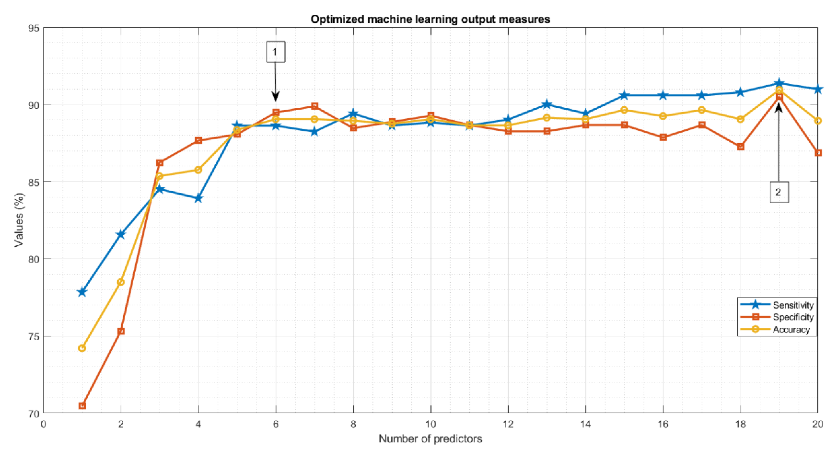
| Optimized ML [6 features] | 89.04 | 0.89 | 88.62 | 89.47 | Ensemble |
| Optimized ML [19 features] | 90.93 | 0.90 | 91.37 | 90.48 | Gaussian SVM |
Publisher’s Note: MDPI stays neutral with regard to jurisdictional claims in published maps and institutional affiliations. |
© 2022 by the authors. Licensee MDPI, Basel, Switzerland. This article is an open access article distributed under the terms and conditions of the Creative Commons Attribution (CC BY) license (https://creativecommons.org/licenses/by/4.0/).
Share and Cite
Keihani, A.; Sajadi, S.S.; Hasani, M.; Ferrarelli, F. Bayesian Optimization of Machine Learning Classification of Resting-State EEG Microstates in Schizophrenia: A Proof-of-Concept Preliminary Study Based on Secondary Analysis. Brain Sci. 2022, 12, 1497. https://doi.org/10.3390/brainsci12111497
Keihani A, Sajadi SS, Hasani M, Ferrarelli F. Bayesian Optimization of Machine Learning Classification of Resting-State EEG Microstates in Schizophrenia: A Proof-of-Concept Preliminary Study Based on Secondary Analysis. Brain Sciences. 2022; 12(11):1497. https://doi.org/10.3390/brainsci12111497
Chicago/Turabian StyleKeihani, Ahmadreza, Seyed Saman Sajadi, Mahsa Hasani, and Fabio Ferrarelli. 2022. "Bayesian Optimization of Machine Learning Classification of Resting-State EEG Microstates in Schizophrenia: A Proof-of-Concept Preliminary Study Based on Secondary Analysis" Brain Sciences 12, no. 11: 1497. https://doi.org/10.3390/brainsci12111497
APA StyleKeihani, A., Sajadi, S. S., Hasani, M., & Ferrarelli, F. (2022). Bayesian Optimization of Machine Learning Classification of Resting-State EEG Microstates in Schizophrenia: A Proof-of-Concept Preliminary Study Based on Secondary Analysis. Brain Sciences, 12(11), 1497. https://doi.org/10.3390/brainsci12111497