Article

Bayesian Network as a Decision Tool for Predicting ALS Disease

1
Department of Statistics, Amasya University, Amasya 05100, Turkey
2
Department of Statistics, Yildiz Technical University, Istanbul 34220, Turkey
3
Department of Chemistry, Ahi Evran University, Kirsehir 40200, Turkey
4
Department of Molecular Biology and Genetics, Yildiz Technical University, Istanbul 34220, Turkey
*
Author to whom correspondence should be addressed.
Brain Sci. 2021, 11(2), 150; https://doi.org/10.3390/brainsci11020150
Submission received: 21 December 2020 / Revised: 9 January 2021 / Accepted: 20 January 2021 / Published: 23 January 2021
(This article belongs to the Collection Collection on Molecular and Cellular Neuroscience)

Abstract

:
Clinical diagnosis of amyotrophic lateral sclerosis (ALS) is difficult in the early period. But blood tests are less time consuming and low cost methods compared to other methods for the diagnosis. The ALS researchers have been used machine learning methods to predict the genetic architecture of disease. In this study we take advantages of Bayesian networks and machine learning methods to predict the ALS patients with blood plasma protein level and independent personal features. According to the comparison results, Bayesian Networks produced best results with accuracy (0.887), area under the curve (AUC) (0.970) and other comparison metrics. We confirmed that sex and age are effective variables on the ALS. In addition, we found that the probability of onset involvement in the ALS patients is very high. Also, a person’s other chronic or neurological diseases are associated with the ALS disease. Finally, we confirmed that the Parkin level may also have an effect on the ALS disease. While this protein is at very low levels in Parkinson’s patients, it is higher in the ALS patients than all control groups.

1. Introduction

Amyotrophic lateral sclerosis (ALS) is a rare neurological disorder mainly caused by progressive degeneration of upper and lower motor neurons. Currently, it is not possible to cure or stop the progression of this disease [1]. ALS may initially affect only one hand or only one leg, making it difficult to walk in a straight line. As the disease progresses, severe muscle weakness, decrease in muscle mass, impaired speech, swallow, fine and gross motor function, and respiratory weakness occur in patients. These lead to paralysis and death usually within 2–5 years following diagnosis [2].
ALS is a multifactorial disease. Approximately 10% of ALS cases are familial (fALS) and 90% of cases are sporadic (sALS) [3]. Although its etiology largely unknown, mutations in various genes have been associated to the ALS [4,5]. There are also some underlying biochemical mechanisms have been proposed, such as protein aggregation, endoplasmic reticulum stress, oxidative stress, mitochondrial impairment, neuro-inflammation, apoptotic cell death, glutamate excitotoxicity, abnormalities in RNA mechanisms, and abnormal function of ubiquitin–proteasome system (UPS) [6].
ALS is typically an adult-onset disease although juvenile forms are present. There are sex-dependent differences in disease development with a slight male predominance [7,8]. ALS can occur in people from all over the world from all ranks of people. Geographical variations have been reported by different population-based studies for the incidence of ALS which ranges 0.6 to 11 cases per 100.000 per year. The prevalence of ALS is between 4.1 and 8.4 per 100.000 persons (reviewed in [9]).
Clinical diagnosis of ALS is difficult in the early period because the patients may not show any upper or lower motor neuron signs [10]. In addition ALS symptoms can be quite heterogeneous and show resemblance to many neurological diseases. Currently the diagnosis is made according to El Escorial Criteria of the World Federation of Neurology and based on complete neurological examination, radiological and electrophysiological investigations [11]. All of these tests may take 3–6 months and cause delay between emergence of early symptoms and diagnosis. It will be possible to prolong the patient’s survival and improve the quality of life with more effective and earlier diagnosis of ALS.
Blood tests are less time consuming and low cost methods compared to other methods for the diagnosis. In addition, the relationship between the values obtained with these analyzes and other variables are very important. This study aims to develop a statistical machine learning model for the prediction of risk of ALS using Parkin protein concentration in blood plasma. For this purpose data was obtained from an experimental study investigating the potential use of Parkin protein as biomarker for the diagnosis of ALS. Patient’s records including age, gender, disease onset, chronic disease information were also obtained from the same study. In this paper, (1) we developed a predictive model using Bayesian networks, (2) examined model performance by comparison with other machine learning methods and (3) created queries based on patient type for evaluation of afore-mentioned variables. In the literature, machine learning methods have been used to examine the genetic architecture of the ALS disease [12]. This study is the first in the literature with its specified features.

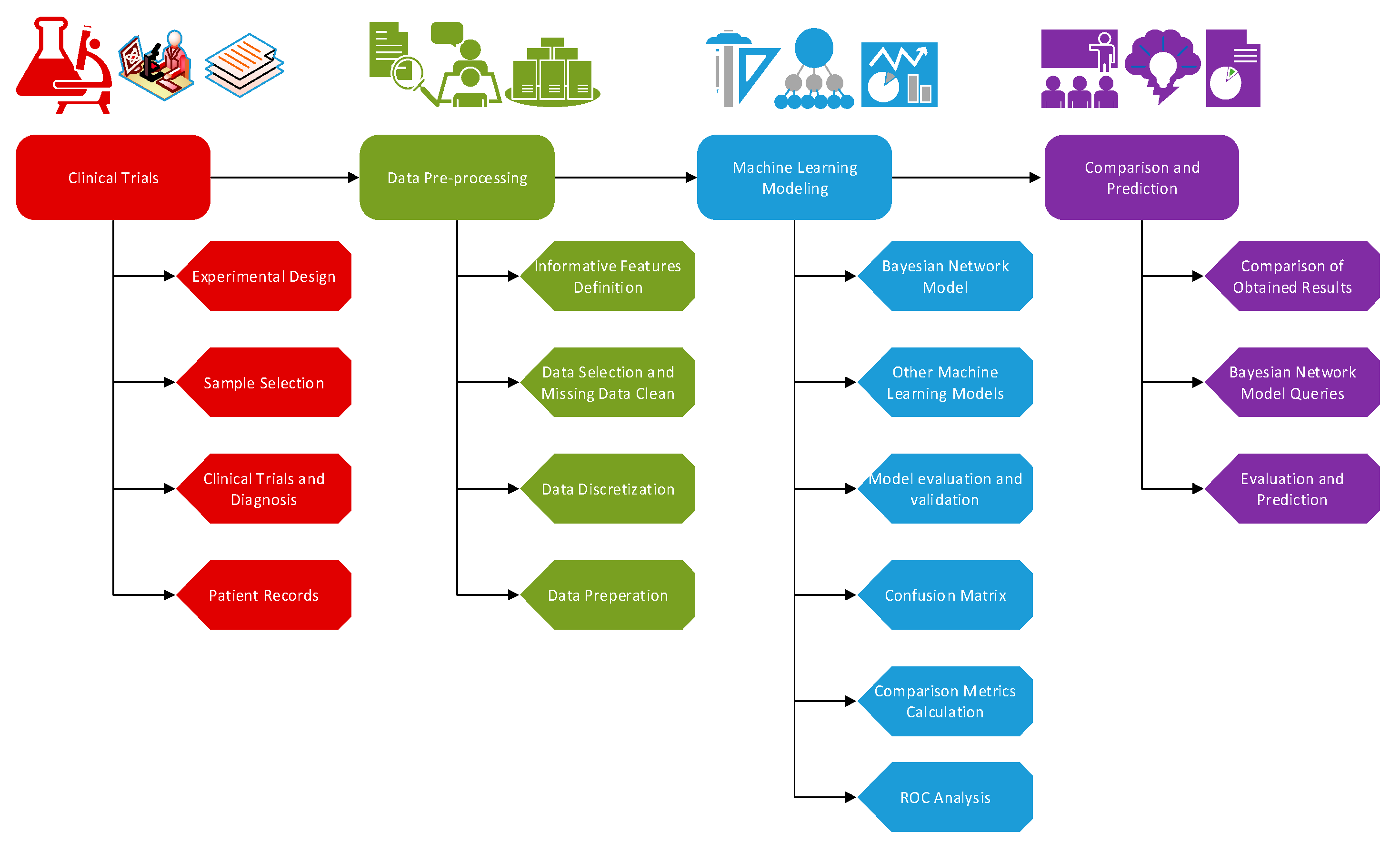
2. Materials and Methods
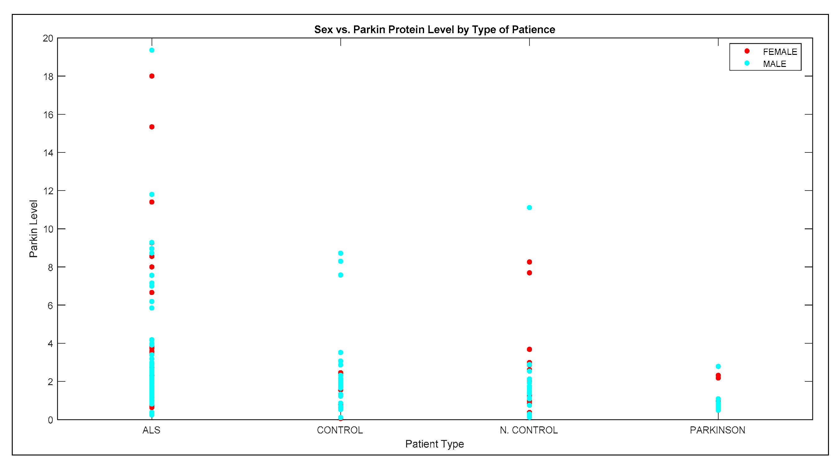
In this section, we summarized the data used in the study and explained the basic steps of the experimental design of machine learning methods used to classify and predict the ALS with ALS-related feature interactions. We described the application process of the study in Figure 1.
In Figure 1, first step was clinical trials to obtain experimental data. Second step, after the properties related to ALS were determined, was data pre-processing. In the next step, the data were modeled with Bayesian networks and other machine learning algorithms, and obtained results were compared. Considering the comparison results, last step was evaluation.

2.1. Participants

This data set has been obtained from an experimental study investigating the differences on the level of Parkin protein between blood plasma from the ALS patients and other neurological cases including multiple sclerosis, frontal dementia and Parkinson’s disease. There is no missing data in the data set, as the patients amnesia was taken in detail.
The characteristics of the subjects used in the study are given in the Table 1. We confirmed that, sex, age, upper motor neurons (UMN), lower motor neurons (LMN), Bulbar onset types, total number of chronic patience and Parkin level (ng/mL) are related to disease type. Accordingly, 50.5% of the data in the study are from the ALS and 9.3% are from Parkinson’s patients. The Neurological Control (N-Control) group includes people with different neurological diseases other than these diseases. Control group consists of completely healthy individuals. Totally 204 individuals are included. All patients were diagnosed and treated by neurologists at Istanbul Medical University according to El Escorial criteria [11].

2.2. Bayesian Networks

Bayesian networks are a graphical modeling approach that models the conditional probabilistic relationships of certain independent variables. In a Bayes network model, nodes correspond to variables, while arrows between nodes show the direct dependency structure between these variables [13]. The direction of the arrow also indicates the direction of the impact.
The probability table for any given X node in the network expresses the values given as X = x for the states of the parents of the node.
P ( X ) = P ( X 1 X n ) = i = 1 n P ( X i | P a ( X i ) )
These networks are widely used in medicine and biology [14,15,16,17]. Bayesian networks are very useful in terms of ease of use of posterior probabilities especially in risk assessment studies [17,18]. The ability to refine the network for new information makes the network more useful and adaptive [19]. In addition, it provides to combine the relationships and expert knowledge stated in the literature with the probabilities obtained from the data as a prior probability. In this respect, it is superior to other machine learning methods [20]. Bayesian networks, which are statistically very strong due to the fact that they are based on probability theory. They are accepted as hybrid methods hence they use both classical statistical techniques and heuristic algorithms [21].

2.3. Other Machine Learning Methods

Machine learning (ML) methods are a subfield of artificial intelligence (AI) and are becoming increasingly common in clinical research [12,22]. The ML methods are mainly examined in three main categories as semi-supervised, supervised and unsupervised algorithms [23]. Supervised learning methods aim to make predictions about unknown situations (e.g., disease type) based on known situations like age, gender, type of onset [12,23]. Classification, similarity detection and regression are among the most common tasks of supervised machine learning methods [24].
In our study, we examined the following seven popular supervised machine learning techniques with Bayesian Network: Artificial Neural Networks, Logistic Regression, Naïve Bayes Algorithm, J48 Algorithm, Support Vector Machines, KStar Algorithm, and K-Nearest Neighbor Algorithm. We investigate as extensively as possible in terms of computing the best results for each machine learning method.
Artificial Neural Network (ANN), based on its learning and generalization abilities, is one of the learning methods that imitate the human brain. These models basically have a hidden layer and input and output layer. One of the most important advantages is that it works on nonlinear, complex models and missing data. Models are optimized with back propagation algorithms of faults during training. On the other hand, lack of rigid hypotheses found in statistical methods makes the ANN advantageous in modeling [25,26].
Logistic regression (LR) is one of the most widely used methods in biology and health science applications [27]. The LR differs from standard regression models due to the structure of the dependent variable. However, as in linear regression models, the relationships of dependent and independent variables are investigated in the LR. The most important difference here is that the dependent variable in LR is dichotomous. In terms of application, the LR is similar to standard linear regression [28]. In cases where there are more than two situations, the LR can be applied to estimate the dependent variable [29].
Naïve Bayes (NB) Algorithm is one of the most important machine learning methods based on Bayes Rule. This method is a classical Bayesian network based on the independence of variables. Classes to be estimated in the NB method must be independent from each other [30]. This method is one of the supervised learning algorithms. Despite being simple, it produces very successful results in medical applications [31,32].
J48 algorithm is one of the most important decision tree algorithms decision trees include popular machine learning algorithms [33]. This algorithm is a modified version of ID3 [34] and c4.5 algorithms [35,36]. While this algorithm uses c4.5, c5.0, and ID3 algorithms to create the decision tree, criteria such as gini index, information gain or entropy reduction are used for estimation [33,36]. Another important feature of it is that it can make predictions by creating a smaller tree compared to other decision trees. This enables the J48 algorithm to produce more successful results than its counterparts [37].
Support Vector Machines (SVMs) are statistical algorithms that use statistical learning theory to produce a consistent estimator using available data [25]. It tries to divide the data into two basic categories. The n-dimensional hyperplane is produced for this reason [38]. Basically, if linear separation of data is possible, system optimization is done the linear SVM. If not possible, quadratic optimization is provided with the non-linear SVM [38,39,40]. Models use kernel functions for this. The selected kernel function affects the performance of the system. Different results can be obtained with different kernel functions.
KStar algorithm is one of the Instance-based learning algorithms in the WEKA program [41]. It is a method that automatically reveals the number of clusters when the number of clusters is unknown [42]. This algorithm uses entropy as a measure of distance [43]. In this respect, the algorithm is similar to the kNN algorithm that uses entropy as a measure of the distance of the data [44].
The k-Nearest Neighbor Algorithm (k-NN) determines the classification of data according to its closest neighbors. This algorithm is one of the most popular algorithms in data mining work [41]. It is preferred because of simplicity and ease of understandability [45]. The similarity function with the k parameter value in the algorithm affects the performance [46]. It calculates the probability of a data considered to be included in the class of its neighbors based on the status of its nearest neighbor. In this respect, it is superior to NN, which is a completely black box. However, it is difficult to determine the distance between neighbors [25].

2.4. Classification Criteria

There are a variety of criteria that can be used to compare the performance of the ML models, the choice of which depends on the structure of the data and nature of the task [12,38,41]. In our study, the numbers of samples in each class are different from each other. In addition, while there are generally two classes in the ML studies, we had four different classes in this study. Increasing the number of classes can affect the results [47]. Since some methods used to evaluate the results are susceptible to unbalanced data, criteria such as Geometric Mean and Youden’s index were also used in the evaluation [48].
The criteria used to determine the algorithms that are effective in this section are given in the Table 2. These criteria were given as Accuracy (ACC), Geometric Mean (GM), Error Rate (ERR), Precision (PREC), Sensitivity (SENS), Specificity (SPEC), F-Measure (FM), Matthew’s correlation coefficient (MCC), Youden’s index (YI), Kappa (κ), False Positive Rate (FPR), and Receiver Operating Characteristic (ROC) Area. Calculation of these formulas is possible by using True positive (TP), True negative (TN), False positive (FP), and False negative (FN) values. Given TP; correct positive prediction, FP; incorrect positive prediction, TN; correct negative prediction, and FN; incorrect negative prediction values are obtained from confusion matrixes.
Accuracy reflects the ratio of true positive and true negative predictions within the total model estimates. The geometric mean is a metric that determines the balance between the results of both the majority and minority subgroups in classification [49]. Accuracy is affected by the changes in the class distribution, but geometric mean is not. For this reason geometric mean is more suitable for the imbalanced dataset [48]. The error rate is complementary to the accuracy. Unlike the measure of accuracy, this metric shows the number of misclassified samples for both positive and negative classes. Precision represents how many positive predictions were genuinely positive for the model. Sensitivity and specificity, representing true positive and true negative rates, are complementary to each other. Sensitivity, also known as the true positive rate, is the ratio of the number of correct positive samples to the number classified as positive, while specificity is the ratio calculated in the same way for negative samples [50].
The equilibrium between precision and sensitivity is represented by the F-Measure. Higher F-Measure indicates good classifier performance. This value is also equal to the harmonic mean of sensitivity and precision [51]. The Matthew’s correlation coefficient is the comparison coefficient that is least affected by unbalanced data and calculates the correlation between observed and predicted classifications. Youden’s index assesses the misclassifications potential of a classifier. The accuracy that can be obtained entirely by chance is calculated by Kappa [52].
The Receiver Operating Curve plots the sensitivity against 1-Specificity to determine an appropriate balance between true and false positive rates. ROC curve is one of the important comparison criteria in clinical studies. This method uses the area under the curve drawn in comparing the subclasses. The larger sum of the AUC shows better classification results [53].
Also, 5-fold cross validation has been preferred for generating estimation results in analyzes. The available data was divided into five, the first four pieces were used for educational purposes and the last piece was used for testing [51]. 5-fold cross-validation is one of the commonly used validation methods to increase model robustness [22].

3. Results

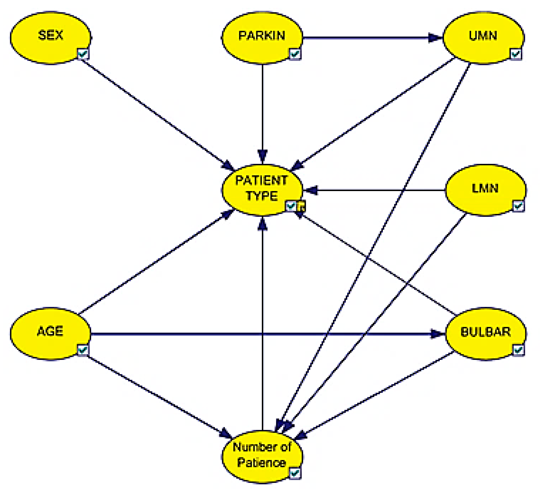
3.1. Bayesian Network Model

The Bayesian network model obtained from the data used is given in Figure 2. Arrows show the relationship between variables in the network. The direction of the arrow also indicates the direction of the impact. The network was created using GeNIe 2.1 Academic version. GeNIe is a machine learning program based on Bayesian networks [54].
According to the Bayesian network model, the types of involvement, age, gender, Parkin protein density and the number of diseases directly affect the type of disease. In addition, it is observed that the types of involvement affect the number of diseases. Since there is at least one disease in people except the control group, it is expected that the involvement will affect the number of diseases. It is known that one of the most important symptoms in the ALS disease is UMN involvement. In the model we obtained as a result of the analysis, it was observed that the Parkin protein density affects the UMN involvement.

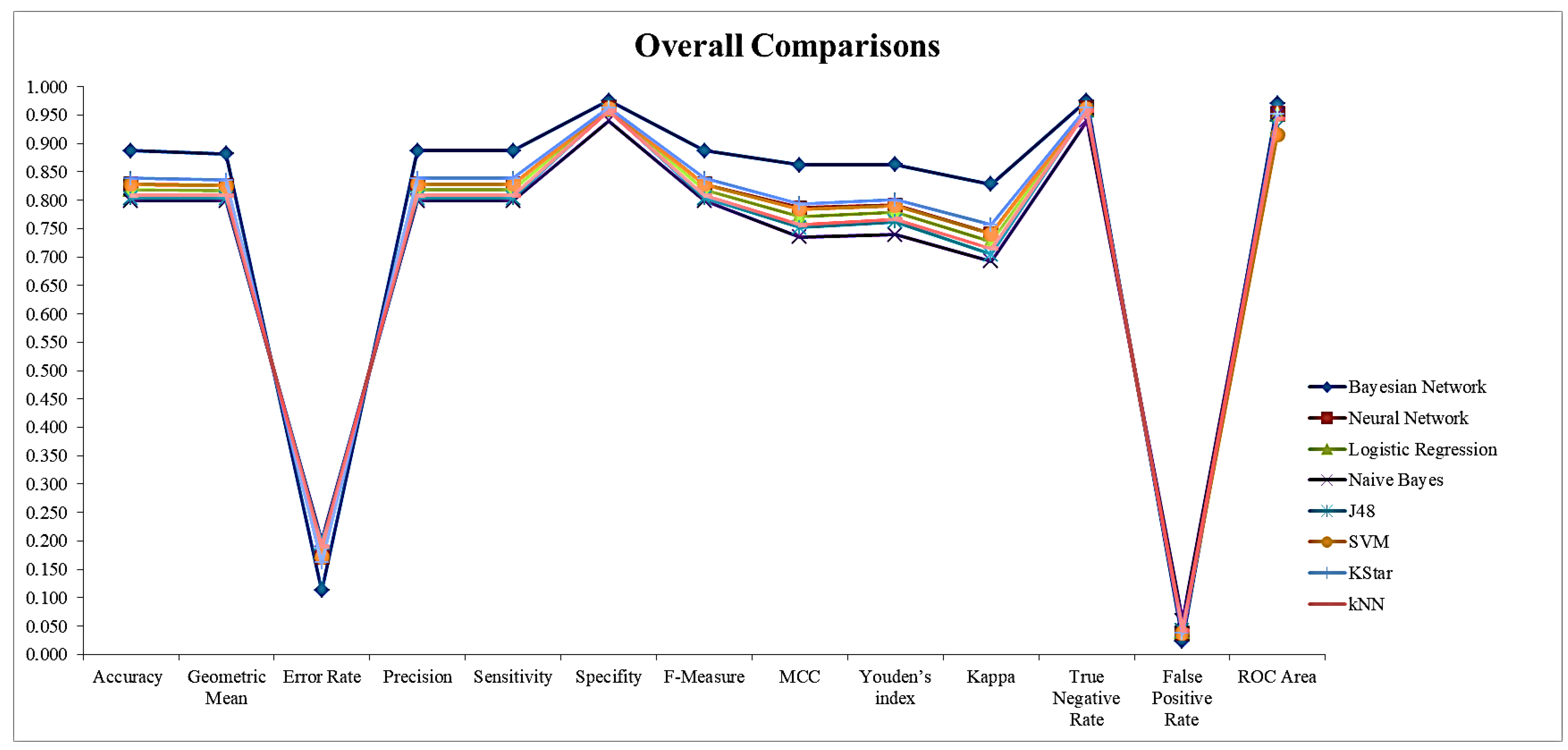
3.2. Comparison Results of Methods

Other machine learning programs that were utilized for comparison were obtained with the WEKA program. This program is Java-based open source software, created by the University of Waikato to facilitate the realization of the ML algorithms [41].
Classification performances of the algorithms according to the classification criteria stated previously are given in Table 3 and Table 4. The generalized results are shown in Table 3 and the results obtained for each class are shown in Table 4. The best classification results according to the criteria are marked in bold.
When the results are examined in general, it has been seen that Bayesian network produces more successful results than other methods. It has been revealed that the Bayes network classifications with little differences. On the other hand, it has been observed that the results of other machine learning methods were close to each other. Polykernel is used for the SVM. For the k-NN, it was seen that the most successful result was obtained with the closest 1 neighbor.
When Table 3 is examined, it is seen that the ACC of Bayesian network is 88.7%. It is observed that the success rates of other methods are approximately 80%. Since Sensitivity and Precision values are the same in the general comparison table, precision values are not included in the table. Specificity value, which expresses confidence in results, shows correctly positively classified variables [55] and this ratio gave high values in all methods. However, the lowest false positive classification rate (0.024) was obtained with Bayesian networks. The same results are also valid for the weighted ROC value.
Graphical comparison of the results is given in Figure 3. When the graph is examined, it is observed that the compared machine learning methods are close to each other and that Bayesian network produces better results than the compared machine learning algorithms.
Comparison should be made for subclasses as well as general comparison of methods. The results of comparison obtained for each subclass are given in Table 4. Accordingly, Bayes network produced more successful results in the ALS estimation than other methods. It was observed that all individuals in the ALS patient group were classified correctly. The results obtained with the SVM and the NN are also close to these values. It can be proposed that all methods yield successful results in predicting the ALS patients. In addition, it is very important to estimate the individuals in other classes.
When the results for the control group were examined, it has been seen that Bayesian network gives the highest ACC value with 0.917. On the other hand, J48 algorithm produced the best results according to GM (0.902), SENS (0.929), and YI (0.805) criteria. However, Bayesian network showed the best fit (0.747) with Kappa value [56] between data and forecast results. In addition, the best results for other criteria for the control group were produced by the Bayesian network.
Bayesian network has produced more successful results than other methods according to all comparison criteria for the Neurological Control group, as in the ALS group. For this group, the Bayesian Network’s ACC value has been found as (0.902). The Kappa values of other methods indicate that the results obtained are random, while the Kappa value (0.677) was found for Bayesian network.
Similar results to the control group were obtained for the last group, Parkinson. The Kstar algorithm produced the best results according to the GM (0.920), SENS (0.895) and YI (0.841) criteria. However, it has been seen that the results obtained for Bayesian network are close to these values.
The ROC curves and the AUC values of the methods are given in Figure 4. According to these values, the AUC value of Bayesian network for each class is higher than other methods. This result supports the values given in Table 4.

3.3. Queries of Bayesian Network Model

One of the most important features of Bayesian networks is that predictions can be made by creating queries with the information and data available [20]. While the known variables are included as evidence, the predicted variables are taken as target nodes. When a new person in one of the disease groups is considered, the questions about the status of other variables are given in Table 5.
When the probability values given in Table 5 are examined, in the absence of any prior knowledge, probability values of the persons are P(Patient Type = ALS) = 0.340; P(Patient Type = Control) = 0.252; P(Patient Type = Neurological Control) = 0.257 and P(Patient Type = Parkinson) = 0.151. From these given values, the conditional probability value obtained for gender is shown in Equation (2).
P   ( S E X   =   F e m a l e   |   P a t i e n t   T y p e   =   A L S ) =   0.382 P   ( S E X   =   M a l e   |   P a t i e n t   T y p e   =   A L S )   =   0.618
According to this result, it is understood that the ALS disease is seen 62% in men and 38% in women. In addition, the ALS disease is expressed largely as an adult-onset disease in the literature [9]. In this part, it was found that 88.1% of the ALS patients were older than 36 years. Furthermore, it was predicted that 54.8% of the ALS patients and 60.5% of Parkinson’s patients were older than 52 years.
P   ( U M N   =   N o   |   P a t i e n t   T y p e   =   A L S ) =   0.273 P   ( U M N   =   Y e s |   P a t i e n t   T y p e   =   A L S )   =   0.727
when the information given in Equation (3) is examined, it is predicted that 72.7% of the ALS patients have the UMN type onset involvement. In addition, it is understood that 82.2% of the patients do not have the LMN and 85.3% have no bulbar onset involvement. However, it was calculated that there were 3.8% of the ALS patients with no involvement. In summary, the probability of having at least 1 type of onset involvement in the ALS patients was predicted 96.2%.
In Table 5, 25.7% of the ALS patients have at least 1 disease other than their own disease. This probability was 19.4% in Parkinson’s patients. This probability was found to be 11.6% in the control group and 11.7% in the neurological control group. Accordingly, it can be thought that different neurological-chronic diseases are related to neurological diseases such as Parkinson’s or ALS.
Moreover, according to the Parkin level, it is predicted that 75.3% of the ALS patients to be higher than 1.36 (ng/mL). This value is quite different in Parkinson’s patients. When Table 5 is examined, 56.3% of Parkinson’s patients’ Parkin level is lower than 1.36 (ng/mL). Also, Parkin level distribution is given in Figure 5. The protein level differences of the groups are also shown in the graph. Protein level is highest in the ALS patients, but this level is lowest in Parkinson’s patients.

4. Discussion and Conclusions

The use of machine learning methods with personal medical records in medical decision-making processes is increasing. In this study Bayesian network—one of the most beneficial ML method in clinical decision-making—has been used for the prediction of ALS, based on differences in the level of a plasma protein, onset, age, sex, and total number of patience. Then results were compared with some popular ML algorithms. To the best of our knowledge, this is the first performance comparison study for Bayesian network model and the ML models for predicting ALS disease using these variables.
Bayesian Networks are one of the probabilistic expert systems that use probability as a measure of uncertainty in order to obtain a graphical structure that best represents the data [57,58]. Since BN uses all the variables in the model, it is easily used in cases where there is missing data [13,59]. With diagnostic reasoning in BN, it is ensured to make a judgement about the patient and the disease by observing various symptoms [60]. Unlike various rule-based ML methods such as NN, LR, SVM, and BN is a method of inference and reasoning. These features allow making queries that reveal cause-effect relationships between variables in the model [13]. The posterior probability values of the network are updated with every new information acquired in BNs. Therefore, the use of BN in prediction problems produces more effective results [61]. The transparency of all relationships in the network structure makes BN advantageous to other ML methods such as k-nn, NN and LR. In addition, it can produce successful results in cases where the data set is small and the number of variables is high [62]. Discretization is main drawback of the BNs which causes loss of information [63]. However, working with discrete data increases the power of accurate prediction regarding classes [64]. All these features have made BN a preferred method in clinical studies [59,62,65,66,67,68].
In this study, unlike the literature, there are three control groups; Parkinson’s disease, neurological control and healthy individuals in the control group. In this way, a comparative result with different control groups containing a large number of subjects improves the applicability of the study in practice.
According to the results of this study, ALS disease is more likely to be seen in men than in women. Various studies have also indicated that gender is an independent variable affecting ALS along with other demographic factors [5,69,70]. Gender was an influential variable and it was confirmed that the ALS disease is more common in males [7,8,71,72,73]. There are studies showing that there is a difference in onset of the disease in ALS patients with different mutations depending on sex [70,74]. Although it is known in which gene some of ALS patients carry a mutation in this study, it has not been taken into consideration. In the future, a similar analysis can be applied to a more homogeneous ALS patient group in terms of mutation.
It has been determined that with the algorithm used in this study, the probability of having ALS will be higher with increasing age. This finding is also consistent with the results of previous studies [75,76]. UMN, LMN and Bulbar are the onset types seen in ALS disease. The probability of having at least one of each kind of onset involvement in the ALS patients was found to be 96.2%. UMN has been determined to be the most common type of involvement. LMN and Bulbar are less common. ALS patients can present together with each a LMN or UMN prevalent phenotype [77]. Previously particular clinical and demographic characteristics of ALS phenotypes have been demonstrated in a population based study with a large epidemiological setting The likelihood of a specific phenotype occurring in different age and gender groups changes. Bulbar phenotype occurs mostly in elderly patients with almost equal incidence rates in the two genders [76].
In particular, the ALS is considered as a multifactorial disease which influenced by environmental and genetic factors. Other neurological diseases that people have can have a small effect on the ALS. It is thought that brain damages and mutations [77] caused by other diseases such as schizophrenia [78], Alzheimer’s disease, Parkinson’s disease, or frontotemporal dementia [79,80] should be associated with the ALS. In our study, the probability of having multiple diseases with the ALS was higher than the control and neurological control groups. Similar results were seen in Parkinson’s patients. Therefore, it will be beneficial to treat patients considering multiple disease situations.
According to all these results, the algorithms we use and the Bayesian network can predict the correct classes with high accuracy rates when information such as the type of involvement of individuals, Parkin protein level, age, and the number of various chronic diseases are considered. Although other machine learning algorithms also produce results with high success, the most important advantage of Bayesian network in this regard is that it can be updated with new additional information and this aspect increases its success. In this respect, it provides more useful results than other machine learning methods such as artificial neural networks showing black box feature in prospective studies, the change of the results should be examined by increasing number of samples and using more variables. The results obtained from statistical and computational methods may be more useful in combination with neuroimaging methods. There is such a study in the literature [81]. A similar approach can be used to classify images of different brain networks as alternative or additional views and the entire MV framework can be further extended to combine imaging with non-imaging views, such as clinical, behavioral, or even genetic multidimensional data, when available from the same subjects.

Author Contributions

Conceptualization, A.G., S.V.K., R.C., and H.A.K.; methodology, H.A.K. and I.D.; software, H.A.K. and I.D.; validation, A.G., R.C., and S.V.K.; formal analysis, H.A.K.; investigation, A.G., S.V.K., and H.A.K.; resources, H.A.K., A.G., and S.V.K.; data curation, A.G., S.V.K., and R.C.; writing—original draft preparation, H.A.K., A.G. and S.V.K.; writing—review and editing, H.A.K., A.G., and S.V.K.; visualization, H.A.K. All authors have read and agreed to the published version of the manuscript.

Funding

This research received no external funding.

Institutional Review Board Statement

Ethical approvals for this study were acquired from Istanbul University, Faculty of Medicine (2016/665 File number, meeting issue is 10 on 24 May 2016) All volunteers participating the study declared their consent and signed the related ethical documents.

Informed Consent Statement

Informed consent was obtained from all subjects involved in the study.

Acknowledgments

We are deeply grateful to Atilla Halil Idrisoglu for his valuable support in the collection of blood samples.

Conflicts of Interest

The authors declare no conflict of interest.

References

  1. Rowland, L.P.; Shneider, N.A. Amyotrophic Lateral Sclerosis. N. Engl. J. Med. 2001, 344, 1688–1700. [Google Scholar] [CrossRef] [PubMed]
  2. Hardiman, O.; van den Berg, L.H.; Kiernan, M.C. Clinical Diagnosis and Management of Amyotrophic Lateral Sclerosis. Nat. Rev. Neurol. 2011, 7, 639–649. [Google Scholar] [CrossRef] [PubMed]
  3. Swinnen, B.; Robberecht, W. The Phenotypic Variability of Amyotrophic Lateral Sclerosis. Nat. Rev. Neurol. 2014, 10, 661. [Google Scholar] [CrossRef] [PubMed] [Green Version]
  4. Al-Chalabi, A.; Hardiman, O. The Epidemiology of ALS: A Conspiracy of Genes, Environment and Time. Nat. Rev. Neurol. 2013, 9, 617. [Google Scholar] [CrossRef] [PubMed]
  5. Filippini, T.; Fiore, M.; Tesauro, M.; Malagoli, C.; Consonni, M.; Violi, F.; Arcolin, E.; Iacuzio, L.; Oliveri Conti, G.; Cristaldi, A.; et al. Clinical and Lifestyle Factors and Risk of Amyotrophic Lateral Sclerosis: A Population-Based Case-Control Study. Int. J. Environ. Res. Public Health 2020, 17, 857. [Google Scholar] [CrossRef] [PubMed] [Green Version]
  6. Mendonça, D.M.F.; Pizzati, L.; Mostacada, K.; Martins, S.C.D.S.; Higashi, R.; Sá, L.A.; Neto, V.M.; Chimelli, L.; Martinez, A.M.B. Neuroproteomics: An insight into ALS. Neurol. Res. 2012, 34, 937–943. [Google Scholar] [CrossRef]
  7. Manjaly, Z.R.; Scott, K.M.; Abhinav, K.; Wijesekera, L.; Ganesalingam, J.; Goldstein, L.H.; Janssen, A.; Dougherty, A.; Willey, E.; Stanton, B.R.; et al. The Sex Ratio in Amyotrophic Lateral Sclerosis: A Population Based Study. Amyotroph. Lateral Scler. 2010, 11, 439–442. [Google Scholar] [CrossRef]
  8. Pape, J.A.; Grose, J.H. The Effects of Diet and Sex in Amyotrophic Lateral Sclerosis. Revue Neurol. 2020, 176, 301–315. [Google Scholar] [CrossRef]
  9. Longinetti, E.; Fang, F. Epidemiology of Amyotrophic Lateral Sclerosis: An Update of Recent Literature. Curr. Opin. Neurol. 2019, 32, 771. [Google Scholar] [CrossRef]
  10. Le Gall, L.; Anakor, E.; Connolly, O.; Vijayakumar, U.G.; Duddy, W.J.; Duguez, S. Molecular and Cellular Mechanisms Affected in ALS. J. Pers. Med. 2020, 10, 101. [Google Scholar] [CrossRef]
  11. Brooks, B.R.; Miller, R.G.; Swash, M.; Munsat, T.L. El Escorial Revisited: Revised Criteria for the Diagnosis of Amyotrophic Lateral Sclerosis. Amyotroph. Lateral Scler. Other Mot. Neuron Disord. 2000, 1, 293–299. [Google Scholar] [CrossRef] [PubMed]
  12. Vasilopoulou, C.; Morris, A.P.; Giannakopoulos, G.; Duguez, S.; Duddy, W. What Can Machine Learning Approaches in Genomics Tell Us about the Molecular Basis of Amyotrophic Lateral Sclerosis? J. Pers. Med. 2020, 10, 247. [Google Scholar] [CrossRef] [PubMed]
  13. Pearl, J. Probabilistic Reasoning in Intelligent Systems: Networks of Plausible Inference; Revised Second Printing; Morgan Kaufmann: San Francisco, CA, USA, 2014; ISBN 978-0-08-051489-5. [Google Scholar]
  14. Bandyopadhyay, S.; Wolfson, J.; Vock, D.M.; Vazquez-Benitez, G.; Adomavicius, G.; Elidrisi, M.; Johnson, P.E.; OConnor, P.J. Data Mining for Censored Time-to-Event Data: A Bayesian Network Model for Predicting Cardiovascular Risk from Electronic Health Record Data. Data Min. Knowl. Discov. 2015, 29, 1033–1069. [Google Scholar] [CrossRef] [Green Version]
  15. Kanwar, M.K.; Lohmueller, L.C.; Kormos, R.L.; Teuteberg, J.J.; Rogers, J.G.; Lindenfeld, J.; Bailey, S.H.; McIlvennan, C.K.; Benza, R.; Murali, S.; et al. A Bayesian Model to Predict Survival after Left Ventricular Assist Device Implantation. JACC Heart Fail. 2018, 6, 771–779. [Google Scholar] [CrossRef] [PubMed]
  16. Kraisangka, J.; Druzdzel, M.J.; Benza, R.L. A Risk Calculator for the Pulmonary Arterial Hypertension Based on a Bayesian Network. In Proceedings of the BMA@ UAI, New York, NY, USA, 29 June 2016; pp. 1–6. [Google Scholar]
  17. Arora, P.; Boyne, D.; Slater, J.J.; Gupta, A.; Brenner, D.R.; Druzdzel, M.J. Bayesian Networks for Risk Prediction Using Real-World Data: A Tool for Precision Medicine. Value Health 2019, 22, 439–445. [Google Scholar] [CrossRef] [PubMed] [Green Version]
  18. Gupta, A.; Slater, J.J.; Boyne, D.; Mitsakakis, N.; Béliveau, A.; Druzdzel, M.J.; Brenner, D.R.; Hussain, S.; Arora, P. Probabilistic Graphical Modeling for Estimating Risk of Coronary Artery Disease: Applications of a Flexible Machine-Learning Method. Med. Decis. Mak. 2019, 39, 1032–1044. [Google Scholar] [CrossRef] [PubMed]
  19. Lam, W.; Bacchus, F. Learning Bayesian Belief Networks: An Approach Based on the Mdl Principle. Comput. Intell. 1994, 10, 269–293. [Google Scholar] [CrossRef] [Green Version]
  20. Koller, D.; Friedman, N. Probabilistic Graphical Models. Principles and Techniques; MIT Press: Cambridge, MA, USA, 2009. [Google Scholar]
  21. Probabilistic Modeling in Bioinformatics and Medical Informatics; Husmeier, D.; Dybowski, R.; Roberts, S. (Eds.) Advanced Information and Knowledge Processing; Springer: London, UK, 2005; ISBN 978-1-85233-778-0. [Google Scholar]
  22. Senders, J.T.; Staples, P.C.; Karhade, A.V.; Zaki, M.M.; Gormley, W.B.; Broekman, M.L.D.; Smith, T.R.; Arnaout, O. Machine Learning and Neurosurgical Outcome Prediction: A Systematic Review. World Neurosurg. 2018, 109, 476–486. [Google Scholar] [CrossRef]
  23. Deo Rahul, C. Machine Learning in Medicine. Circulation 2015, 132, 1920–1930. [Google Scholar] [CrossRef] [Green Version]
  24. Yu, K.-H.; Beam, A.L.; Kohane, I.S. Artificial Intelligence in Healthcare. Nat. Biomed. Eng. 2018, 2, 719–731. [Google Scholar] [CrossRef]
  25. Dreiseitl, S.; Ohno-Machado, L. Logistic Regression and Artificial Neural Network Classification Models: A Methodology Review. J. Biomed. Inform. 2002, 35, 352–359. [Google Scholar] [CrossRef] [Green Version]
  26. Gevrey, M.; Dimopoulos, I.; Lek, S. Review and Comparison of Methods to Study the Contribution of Variables in Artificial Neural Network Models. Ecol. Model. 2003, 160, 249–264. [Google Scholar] [CrossRef]
  27. Christodoulou, E.; Ma, J.; Collins, G.S.; Steyerberg, E.W.; Verbakel, J.Y.; Van Calster, B. A Systematic Review Shows No Performance Benefit of Machine Learning over Logistic Regression for Clinical Prediction Models. J. Clin. Epidemiol. 2019, 110, 12–22. [Google Scholar] [CrossRef]
  28. Hosmer, D.W., Jr.; Lemeshow, S.; Sturdivant, R.X. Applied Logistic Regression; John Wiley & Sons: Hoboken, NJ, USA, 2013; Volume 398. [Google Scholar]
  29. Kleinbaum, D.G.; Dietz, K.; Gail, M.; Klein, M.; Klein, M. Logistic Regression; Springer: New York, NY, USA, 2002. [Google Scholar]
  30. John, G.; Langley, P. Estimating Continuous Distributions in Bayesian Classifiers. In Proceedings of the Eleventh Conference on Uncertainty in Artificial Intelligence; Morgan Kaufmann: San Mateo, CA, USA, 1995; pp. 338–345. [Google Scholar]
  31. Wei, W.; Visweswaran, S.; Cooper, G.F. The Application of Naive Bayes Model Averaging to Predict Alzheimer’s Disease from Genome-Wide Data. J. Am. Med. Inform. Assoc. 2011, 18, 370–375. [Google Scholar] [CrossRef] [PubMed] [Green Version]
  32. Jiang, W.; Shen, Y.; Ding, Y.; Ye, C.; Zheng, Y.; Zhao, P.; Liu, L.; Tong, Z.; Zhou, L.; Sun, S.; et al. A Naive Bayes Algorithm for Tissue Origin Diagnosis (TOD-Bayes) of Synchronous Multifocal Tumors in the Hepatobiliary and Pancreatic System. Int. J. Cancer 2018, 142, 357–368. [Google Scholar] [CrossRef] [Green Version]
  33. Rokach, L.; Maimon, O. Decision Trees. In Data Mining and Knowledge Discovery Handbook; Maimon, O., Rokach, L., Eds.; Springer US: Boston, MA, USA, 2005; pp. 165–192. ISBN 978-0-387-25465-4. [Google Scholar]
  34. Kaur, G.; Chhabra, A. Improved J48 Classification Algorithm for the Prediction of Diabetes. Int. J. Comput. Appl. 2014, 98, 13–17. [Google Scholar] [CrossRef]
  35. Quinlan, J.R. Improved Use of Continuous Attributes in C4. 5. J. Artif. Intell. Res. 1996, 4, 77–90. [Google Scholar] [CrossRef] [Green Version]
  36. Yadav, A.K.; Chandel, S. Solar Energy Potential Assessment of Western Himalayan Indian State of Himachal Pradesh Using J48 Algorithm of WEKA in ANN Based Prediction Model. Renew. Energy 2015, 75, 675–693. [Google Scholar] [CrossRef]
  37. bin Othman, M.F.; Yau, T.M.S. Comparison of Different Classification Techniques Using WEKA for Breast Cancer. In Proceedings of the 3rd Kuala Lumpur International Conference on Biomedical Engineering 2006, Kuala Lumpur, Malaysia, 11–14 December 2006; Ibrahim, F., Osman, N.A.A., Usman, J., Kadri, N.A., Eds.; Springer: Berlin/Heidelberg, Germany, 2007; pp. 520–523. [Google Scholar]
  38. Alpaydin, E. Introduction to Machine Learning; MIT Press: Cambridge, MA, USA, 2004. [Google Scholar]
  39. Schölkopf, B.; Smola, A.J. Learning with Kernels: Support Vector Machines, Regularization, Optimization, and Beyond; Adaptive Computation and Machine Learning; MIT Press: Cambridge, MA, USA, 2009; ISBN 0-262-19475-9. [Google Scholar]
  40. Cristianini, N.; Shawe-Taylor, J. An Introduction to Support Vector Machines and Other Kernel-Based Learning Methods; Cambridge University Press: Cambridge, UK, 2000; ISBN 0-521-78019-5. [Google Scholar]
  41. Witten, I.H.; Frank, E.; Hall, M.A.; Pal, C.J. Data Mining: Practical Machine Learning Tools and Techniques with Java Implementations, 4th ed.; Morgan Kaufmann Publishers: Burlington, MA, USA, 2017; ISBN 1-55860-552-5. [Google Scholar]
  42. Pinto, D.; Tovar, M.; Vilarino, D.; Beltrán, B.; Jiménez-Salazar, H.; Campos, B. BUAP: Performance of K-Star at the INEX’09 Clustering Task. In Proceedings of the International Workshop of the Initiative for the Evaluation of XML Retrieval, Brisbane, QLD, Australia, 7–9 December 2009; pp. 434–440. [Google Scholar]
  43. Painuli, S.; Elangovan, M.; Sugumaran, V. Tool Condition Monitoring Using K-Star Algorithm. Expert Syst. Appl. 2014, 41, 2638–2643. [Google Scholar] [CrossRef]
  44. Wiharto, W.; Kusnanto, H.; Herianto, H. Intelligence System for Diagnosis Level of Coronary Heart Disease with K-Star Algorithm. Healthc. Inform. Res. 2016, 22, 30–38. [Google Scholar] [CrossRef] [Green Version]
  45. Zhang, S.; Cheng, D.; Deng, Z.; Zong, M.; Deng, X. A Novel KNN Algorithm with Data-Driven k Parameter Computation. Pattern Recognit. Lett. 2018, 109, 44–54. [Google Scholar] [CrossRef]
  46. Filiz, E.; Öz, E. Educational Data Mining Methods For Timss 2015 Mathematics Success: Turkey Case. Sigma J. Eng. Nat. Sci. /Mühendislik ve Fen Bilimleri Dergisi 2020, 38, 963–977. [Google Scholar]
  47. Ballabio, D.; Grisoni, F.; Todeschini, R. Multivariate Comparison of Classification Performance Measures. Chemom. Intell. Lab. Syst. 2018, 174, 33–44. [Google Scholar] [CrossRef]
  48. Tharwat, A. Classification Assessment Methods. Appl. Comput. Inform. 2020. [Google Scholar] [CrossRef]
  49. Kuncheva, L.I.; Arnaiz-González, Á.; Díez-Pastor, J.-F.; Gunn, I.A.D. Instance Selection Improves Geometric Mean Accuracy: A Study on Imbalanced Data Classification. Prog. Artif. Intell. 2019, 8, 215–228. [Google Scholar] [CrossRef] [Green Version]
  50. Marsland, S. Machine Learning: An Algorithmic Perspective, 2nd ed.; CRC Press: Boca Raton, FL, USA, 2015; ISBN 978-1-4665-8333-7. [Google Scholar]
  51. Sakr, S.; Elshawi, R.; Ahmed, A.M.; Qureshi, W.T.; Brawner, C.A.; Keteyian, S.J.; Blaha, M.J.; Al-Mallah, M.H. Comparison of Machine Learning Techniques to Predict All-Cause Mortality Using Fitness Data: The Henry Ford ExercIse Testing (FIT) Project. BMC Med. Inform. Decis. Mak. 2017, 17, 174. [Google Scholar] [CrossRef] [Green Version]
  52. Akosa, J. Predictive Accuracy: A Misleading Performance Measure for Highly Imbalanced Data. In Proceedings of the SAS Global Forum, Oklahoma State University, Orlando, FL, USA, 2–5 April 2017; pp. 2–5. [Google Scholar]
  53. Fawcett, T. An Introduction to ROC Analysis. Pattern Recognit. Lett. 2006, 27, 861–874. [Google Scholar] [CrossRef]
  54. BayesFusion, L. GeNIe Modeler User Manual; BayesFusion, LLC: Pittsburgh, PA, USA, 2017. [Google Scholar]
  55. Powers, D. Evaluation: From Precision, Recall and F-Measure to ROC, Informedness, Markedness & Correlation. J. Mach. Learn. Technol. 2011, 2, 37–63. [Google Scholar]
  56. Viera, A.J.; Garrett, J.M. Understanding Interobserver Agreement: The Kappa Statistic. Fam. Med. 2005, 37, 360–363. [Google Scholar]
  57. Spiegelhalter, D.J.; Dawid, A.P.; Lauritzen, S.L.; Cowell, R.G. Bayesian Analysis in Expert Systems. Stat. Sci. 1993, 8, 219–247. [Google Scholar] [CrossRef]
  58. Jensen, F.V.; Nielsen, T.D. Bayesian Networks and Decision Graphs, 2nd ed.; Information Science and Statistics; Springer: New York, NY, USA, 2007; ISBN 978-0-387-68281-5. [Google Scholar]
  59. Lin, J.-H.; Haug, P.J. Exploiting Missing Clinical Data in Bayesian Network Modeling for Predicting Medical Problems. J. Biomed. Inform. 2008, 41, 1–14. [Google Scholar] [CrossRef] [PubMed]
  60. Korb, K.B.; Nicholson, A.E. Bayesian Artificial Intelligence; CRC Press: Boca Raton, FL, USA, 2011; p. 479. [Google Scholar]
  61. Chen, R.; Herskovits, E.H. Clinical Diagnosis Based on Bayesian Classification of Functional Magnetic-Resonance Data. Neuroinformatics 2007, 5, 178–188. [Google Scholar] [CrossRef] [PubMed]
  62. Luo, Y.; El Naqa, I.; McShan, D.L.; Ray, D.; Lohse, I.; Matuszak, M.M.; Owen, D.; Jolly, S.; Lawrence, T.S.; Kong, F.-M.; et al. Unraveling Biophysical Interactions of Radiation Pneumonitis in Non-Small-Cell Lung Cancer via Bayesian Network Analysis. Radiother. Oncol. 2017, 123, 85–92. [Google Scholar] [CrossRef] [PubMed] [Green Version]
  63. Nojavan, A.F.; Qian, S.S.; Stow, C.A. Comparative Analysis of Discretization Methods in Bayesian Networks. Environ. Model. Softw. 2017, 87, 64–71. [Google Scholar] [CrossRef]
  64. Yang, Y.; Webb, G.I. A Comparative Study of Discretization Methods for Naive-Bayes Classifiers. In Proceedings of the PKAW 2002: The 2002 Pacific Rim Knowledge Acquisition Workshop, Tokyo, Japan, 18–19 August 2002; pp. 159–173. [Google Scholar]
  65. Rodríguez-López, V.; Cruz-Barbosa, R. Improving Bayesian Networks Breast Mass Diagnosis by Using Clinical Data. In Proceedings of the Pattern Recognition, Mexico City, Mexico, 24–27 June 2015; Carrasco-Ochoa, J.A., Martí­nez-Trinidad, J.F., Sossa-Azuela, J.H., Olvera López, J.A., Famili, F., Eds.; Springer International Publishing: Cham, Switzerland, 2015; pp. 292–301. [Google Scholar]
  66. Nagarajan, R.; Scutari, M.; Lèbre, S. Bayesian Networks in R: With Applications in Systems Biology; Use R! Springer: New York, NY, USA, 2013; ISBN 978-1-4614-6445-7. [Google Scholar]
  67. Antal, P.; Fannes, G.; Timmerman, D.; Moreau, Y.; De Moor, B. Using Literature and Data to Learn Bayesian Networks as Clinical Models of Ovarian Tumors. Artif. Intell. Med. 2004, 30, 257–281. [Google Scholar] [CrossRef]
  68. Khanna, S.; Domingo-Fernández, D.; Iyappan, A.; Emon, M.A.; Hofmann-Apitius, M.; Fröhlich, H. Using Multi-Scale Genetic, Neuroimaging and Clinical Data for Predicting Alzheimer’s Disease and Reconstruction of Relevant Biological Mechanisms. Sci. Rep. 2018, 8, 11173. [Google Scholar] [CrossRef] [Green Version]
  69. Palmieri, A.; Mento, G.; Calvo, V.; Querin, G.; D’Ascenzo, C.; Volpato, C.; Kleinbub, J.R.; Bisiacchi, P.S.; Sorarù, G. Female Gender Doubles Executive Dysfunction Risk in ALS: A Case-Control Study in 165 Patients. J. Neurol. Neurosurg. Psychiatry 2015, 86, 574–579. [Google Scholar] [CrossRef]
  70. Trojsi, F.; D’Alvano, G.; Bonavita, S.; Tedeschi, G. Genetics and Sex in the Pathogenesis of Amyotrophic Lateral Sclerosis (ALS): Is There a Link? Int. J. Mol. Sci. 2020, 21, 3647. [Google Scholar] [CrossRef]
  71. Chiò, A.; Moglia, C.; Canosa, A.; Manera, U.; D’Ovidio, F.; Vasta, R.; Grassano, M.; Brunetti, M.; Barberis, M.; Corrado, L.; et al. ALS Phenotype Is Influenced by Age, Sex, and Genetics: A Population-Based Study. Neurology 2020, 94, e802–e810. [Google Scholar] [CrossRef]
  72. Ingre, C.; Roos, P.M.; Piehl, F.; Kamel, F.; Fang, F. Risk Factors for Amyotrophic Lateral Sclerosis. Clin. Epidemiol. 2015, 7, 181–193. [Google Scholar] [CrossRef] [Green Version]
  73. Trojsi, F.; Siciliano, M.; Femiano, C.; Santangelo, G.; Lunetta, C.; Calvo, A.; Moglia, C.; Marinou, K.; Ticozzi, N.; Ferro, C.; et al. Comparative Analysis of C9orf72 and Sporadic Disease in a Large Multicenter ALS Population: The Effect of Male Sex on Survival of C9orf72 Positive Patients. Front. Neurosci. 2019, 13, 485. [Google Scholar] [CrossRef] [PubMed]
  74. Rooney, J.; Fogh, I.; Westeneng, H.-J.; Vajda, A.; McLaughlin, R.; Heverin, M.; Jones, A.; van Eijk, R.; Calvo, A.; Mazzini, L.; et al. C9orf72 Expansion Differentially Affects Males with Spinal Onset Amyotrophic Lateral Sclerosis. J. Neurol. Neurosurg. Psychiatry 2017, 88, 281. [Google Scholar] [CrossRef] [PubMed] [Green Version]
  75. Atsuta, N.; Watanabe, H.; Ito, M.; Tanaka, F.; Tamakoshi, A.; Nakano, I.; Aoki, M.; Tsuji, S.; Yuasa, T.; Takano, H.; et al. Age at Onset Influences on Wide-Ranged Clinical Features of Sporadic Amyotrophic Lateral Sclerosis. J. Neurol. Sci. 2009, 276, 163–169. [Google Scholar] [CrossRef] [PubMed]
  76. Chiò, A.; Calvo, A.; Moglia, C.; Mazzini, L.; Mora, G.; PARALS Study Group. Phenotypic Heterogeneity of Amyotrophic Lateral Sclerosis: A Population Based Study. J. Neurol. Neurosurg. Psychiatry 2011, 82, 740–746. [Google Scholar] [CrossRef] [PubMed]
  77. Connolly, O.; Le Gall, L.; McCluskey, G.; Donaghy, C.G.; Duddy, W.J.; Duguez, S. A Systematic Review of Genotype–Phenotype Correlation across Cohorts Having Causal Mutations of Different Genes in ALS. J. Pers. Med. 2020, 10, 58. [Google Scholar] [CrossRef]
  78. van Es, M.A.; Hardiman, O.; Chio, A.; Al-Chalabi, A.; Pasterkamp, R.J.; Veldink, J.H.; van den Berg, L.H. Amyotrophic Lateral Sclerosis. Lancet 2017, 390, 2084–2098. [Google Scholar] [CrossRef]
  79. Nguyen, H.P.; Van Broeckhoven, C.; van der Zee, J. ALS Genes in the Genomic Era and Their Implications for FTD. Trends Genet. 2018, 34, 404–423. [Google Scholar] [CrossRef] [Green Version]
  80. Andersen, P.M.; Al-Chalabi, A. Clinical Genetics of Amyotrophic Lateral Sclerosis: What Do We Really Know? Nat. Rev. Neurol. 2011, 7, 603–615. [Google Scholar] [CrossRef]
  81. Fratello, M.; Caiazzo, G.; Trojsi, F.; Russo, A.; Tedeschi, G.; Tagliaferri, R.; Esposito, F. Multi-View Ensemble Classification of Brain Connectivity Images for Neurodegeneration Type Discrimination. Neuroinform 2017, 15, 199–213. [Google Scholar] [CrossRef] [Green Version]
Figure 1. Modeling process with machine learning methods.
Brainsci 11 00150 g001
Figure 2. Bayesian network model of dataset.
Brainsci 11 00150 g002
Figure 3. Overall comparison of methods.
Brainsci 11 00150 g003
Figure 4. ROC Analysis Results of Methods; (a) Bayesian Network, (b) Neural Network, (c) Logistic Regression, (d) Naive Bayes, (e) J48, (f) SVM, (g) KStar, (h) kNN.
Brainsci 11 00150 g004aBrainsci 11 00150 g004b
Figure 5. Sex vs. Parkin level (ng/mL) by the type of disease.
Brainsci 11 00150 g005
Table 1. Characteristics of patients.
Feature NameFeature ValueFreq.%Value
SEXFemale7938.7
Male12561.3
AGEBelow 362914.2
Between 36–527034.3
Between 52–677938.7
Upper 672612.7
UMNNo12963.2
Yes7536.8
LMNNo17887.3
Yes2612.7
BULBARNo18289.2
Yes2210.8
Total Number of Chronic PatienceFive10.5
Four10.5
Three125.9
Two209.8
One11254.9
None5828.4
PARKIN Level (ng/mL)Upper than 3.743115.2
Between 2.79–3.74178.3
Between 2.06–2.793617.6
Between 1.36–2.065225.5
Lower than 1.366833.3
Patient typeALS10350.5
Control4220.6
N-Control4019.6
Parkinson199.3
Table 2. Evaluation criteria formulas.
CriteriaFormula
AccuracyACC = (TP + TN)/(P + N)
Geometric MeanGM = sqrt ((TP/(TP + FN)) × (TN/(TN + FP)))
Error RateEER = (FP + FN)/(TP + TN + FP + FN)
PrecisionPREC = TP/(TP + FP)
SensitivitySENS = TP/(TP + FN)
SpecificitySPEC = TN/(FP + TN)
F-MeasureF-Measure = 2 × TP/(2 × TP + FP + FN)
Matthews Correlation CoefficientMCC = TP × TN − FP×FN/sqrt((TP + FP) × (TP + FN) × (TN + FP) × (TN + FN))
Youden’s indexYI = TPR + TNR − 1
KappaKappa = 2 × (TP × TN – FN × FP) / (TP × FN + TP × FP + 2 × TP × TN + FN2 + FN × TN + FP2 + FP × TN)
Overall KappaKappa = (p0 − pe)/(1 − pe)
p0 = observed accuracy; pe = expected accuracy
False Positive RateFPR = FP/(FP + TN)
Table 3. Overall comparisons for methods.
ACCGMERRSENSSPECF-MMCCYIKappaFPRROC
Bayesian Network0.8870.8820.1130.8870.9760.8870.8620.8630.8280.0240.970
Neural Network0.8280.8260.1720.8280.9630.8280.7870.7910.7410.0370.953
Logistic Regression0.8190.8170.1810.8190.9600.8190.7720.7780.7270.0400.951
Naive Bayes0.7990.8000.2010.7990.9400.7990.7360.7390.6930.0600.951
J480.8040.8040.1960.8040.9580.8040.7520.7620.7050.0420.930
Support Vector Machine (SVM)0.8280.8260.1720.8280.9620.8280.7840.7900.7410.0380.916
KStar0.8380.8350.1620.8380.9630.8380.7940.8010.7560.0370.952
k-Nearest Neighbor (k-NN)0.8090.8080.1910.8090.9580.8090.7560.7660.7150.0420.943
Table 4. Comparisons of Methods for ALS, Control, Neurological Control and Parkinson Disease.
ACCGMERRPRECSENSSPECF-MMCCYIKappa
ALSBayesian Network1.0001.0000.0001.0001.0001.0001.0001.0001.0001.000
Neural Network0.9850.9850.0151.0000.9711.0000.9850.9710.9710.971
Logistic Regression0.9750.9750.0251.0000.9511.0000.9750.9520.9510.951
Naive Bayes0.9710.9700.0290.9620.9810.9600.9710.9410.9410.941
J480.9800.9800.0201.0000.9611.0000.9800.9620.9610.961
SVM0.9800.9800.0201.0000.9611.0000.9800.9620.9610.961
Kstar0.9750.9760.0250.9900.9610.9900.9750.9510.9510.951
k-NN0.9560.9560.0440.9900.9220.9900.9550.9140.9120.912
ControlBayesian Network0.9170.8740.0830.7910.8100.9440.8000.7470.7540.747
Neural Network0.8820.8130.1180.7140.7140.9260.7140.6400.6400.640
Logistic Regression0.8680.8450.1320.6420.8100.8830.7160.6380.6920.631
Naive Bayes0.8820.8540.1180.6800.8100.9010.7390.6680.7110.664
J480.8870.9020.1130.6610.9290.8770.7720.7180.8050.700
SVM0.8920.8970.1080.6790.9050.8890.7760.7190.7940.706
KStar0.9070.8880.0930.7350.8570.9200.7910.7350.7770.732
k-NN0.9120.8910.0880.7500.8570.9260.8000.7460.7830.744
Neurological ControlBayesian Network0.9020.8160.0980.7780.7000.9510.7370.6780.6510.677
Neural Network0.8480.7380.1520.6150.6000.9090.6080.5130.5090.513
Logistic Regression0.8480.6680.1520.6550.4750.9390.5510.4710.4140.462
Naive Bayes0.8090.5680.1910.5190.3500.9210.4180.3170.2710.309
J480.8190.5320.1810.5710.3000.9450.3930.3200.2450.299
SVM0.8430.6500.1570.6430.4500.9390.5290.4490.3890.439
KStar0.8530.6700.1470.6790.4750.9450.5590.4850.4200.474
k-NN0.8330.6610.1670.5940.4750.9210.5280.4320.3960.428
ParkinsonBayesian Network0.9560.9030.0440.7270.8420.9680.7800.7590.8100.756
Neural Network0.9410.8690.0590.6520.7890.9570.7140.6860.7460.682
Logistic Regression0.9460.8980.0540.6670.8420.9570.7440.7210.7990.715
Naive Bayes0.9360.8400.0640.6360.7370.9570.6830.6500.6940.648
J480.9220.8320.0780.5600.7370.9410.6360.6000.6770.593
SVM0.9410.8420.0590.6670.7370.9620.7000.6690.6990.667
KStar0.9410.9200.0590.6300.8950.9460.7390.7210.8410.707
k-NN0.9170.8570.0830.5360.7890.9300.6380.6070.7190.593
Table 5. Bayesian network model queries for patient type.
Target Node (s)Target ValueEvidence (Patient Type)
ALSControlN-ControlParkinson
NoneNone0.3400.2520.2570.151
AGEBelow 360.1190.2490.1060.078
Between 36–520.3330.4190.2980.316
Between 52–670.4370.2320.4490.430
Upper 670.1110.1000.1480.175
SEXFemale0.3820.3420.4010.452
Male0.6180.6580.5990.548
PARKIN Level (ng/mL)Upper than 3.740.2440.1070.0980.114
Between 2.79–3.740.0780.0720.1000.084
Between 2.06–2.790.1920.2000.1590.131
Between 1.36–2.060.2380.2790.3400.107
Lower than 1.360.2470.3430.3030.563
UMNNo0.2730.8400.8440.733
Yes0.7270.1600.1560.267
LMNNo0.8220.9120.9130.852
Yes0.1780.0880.0870.148
BULBARNo0.8530.9240.9250.872
Yes0.1470.0760.0750.128
Total Number of PatienceNone0.0400.6960.2880.075
One0.7040.1890.5950.731
Two0.1400.0600.0590.101
Three0.1030.0420.0450.070
Four0.0080.0080.0070.013
Five0.0060.0060.0060.010
Publisher’s Note: MDPI stays neutral with regard to jurisdictional claims in published maps and institutional affiliations.

