Article

A Novel Indirect Calibration Approach for Robot Positioning Error Compensation Based on Neural Network and Hand-Eye Vision

1
School of Mechanic and Automotive Engineering, University of Ulsan, Daehak-ro 93, Nam-gu, Ulsan 44610, Korea
2
Abeosystem Co, LTD, Daehak-ro 93, Nam-gu, Ulsan 44610, Korea
*
Author to whom correspondence should be addressed.
Appl. Sci. 2019, 9(9), 1940; https://doi.org/10.3390/app9091940
Submission received: 16 April 2019 / Revised: 4 May 2019 / Accepted: 9 May 2019 / Published: 11 May 2019

Abstract

:

Featured Application

This study aims to improve the absolute position error of robot manipulators for vehicle assembly line without using an expensive external apparatus.

Abstract

It is well known that most of the industrial robots have excellent repeatability in positioning. However, the absolute position errors of industrial robots are relatively poor, and in some cases the error may reach even several millimeters, which make it difficult to apply the robot system to vehicle assembly lines that need small position errors. In this paper, we have studied a method to reduce the absolute position error of robots using machine vision and neural network. The position/orientation of robot tool-end is compensated using a vision-based approach combined with a neural network, where a novel indirect calibration approach is presented in order to gather information for training the neural network. In the simulation, the proposed compensation algorithm was found to reduce the positional error to 98%. On average, the absolute position error was 0.029 mm. The application of the proposed algorithm in the actual robot experiment reduced the error to 50.3%, averaging 1.79 mm.

1. Introduction

The repeated and monotonous manual work is continuously reintegrated by flexible manufacturing systems. To build a flexible manufacturing system, adopting an intelligent robot system is essential to distinguish workpieces within a workspace, perceive a situation and manipulate themselves autonomously [1]. Among the intelligent robot systems, vision-based robot systems have been developed continuously to improve the quality and efficiency of the manufacturing system such as arc welding, materials handling, painting and even assembly [2,3,4]. Especially, picking up an object and assembling it to another subsystem accurately is the most important task in an automated manufacturing system [5,6,7]. To do this task correctly, a robot should be calibrated precisely in advance, and then the robot should be connected with visual sensing systems to observe objects and compute the poses of objects. Although industrial robots generally have high-precision repeatability, the absolute position accuracy of them is not so high due to the kinematic error or assembly tolerance of the robot mechanism [8,9]. In order to improve accuracy, various approaches have been proposed in the literature based on choosing a mathematical error model for robot calibration. From the actual robot experiment, the partial pose or whole pose data of the robot end-effector is gathered, and then it is used to estimate the real robot kinematic parameters. However, the processes of robot calibration considered in the methods are complex, and high precision measurement devices are required to track the nominal pose and the real pose of the robot end-effector. For small-range 3D measurements, touch probes or telescoping-ball bar devices are commonly used. On the other hand, for large-range measurement camera-based systems, coordinate measuring machines (CMM) and laser trackers are typically used [10,11,12,13,14]. However, these types of devices are very expensive to be implemented in robot calibration, and even ineffective.
The conventional robot calibration is often implemented with these convenient devices, but there are still some remaining issues. In fact, the cost of measurement devices and the complexity of the mathematical error model are one of the concerns in the production line. Furthermore, these approaches directly track the pose of the robot end-effector with respect to the device’s coordinate and estimate the robot base coordinate by applying the inverse kinematic process. However, this approach does not guarantee high calibration accuracy. In addition, for the vision-based robot system in the industrial field environment, it is essentially desirable that the system is capable of performing calibration without any expensive external apparatus or elaborate setups, which is the system self-calibration [5,6].
Lots of work about robot calibration techniques without using expensive external devices are reported in the literature. Meng et al. [15] proposed a method for robot calibration using vision technology. This approach only requires a ground-truth scale in the reference frame to estimate the pose of the manipulator. However, the proposed method adopts corner detection to extract the corners of the chessboard; its algorithm is easily affected by noise, leading to the failure of corner detection. Then, calibration errors are increased. Gong et al. [16] proposed a method for calibrating and compensating the robot system kinematic error using its internal laser sensor based on distance measurements. However, this approach is restricted by the sensor accuracy not using the absolute position measurement system to measure the robot end-effector. On the other hand, Yin et al. [17] presented an approach for evaluating the kinematic errors of the robot based on the fixed-point constraints to estimate the robot’s end-effector. The method is limited to aligning the tool-center-point (TCP) of a robot to fixed points in the robot workspace. The predicted position of the robot’s end-effector estimated by the fixed-point and the laser stripe could be misaligned. These techniques are often inconvenient, time consuming and it may not be feasible for some certain applications. To overcome the above limitations, we develop a novel and flexible indirect calibration method for the vision-based robot application that need small position errors. This is a straightforward and efficient method to reduce the absolute position error. Our method does not require the complex solution of the kinematics parameter equations and the complicated procedures of the traditional robot compensation methods. As a result, we successfully reduced the absolute position error the robot’s end-effector in the workspace, the position/orientation of the robot’s end-effector is compensated without modifying the parameters of the robot. Using the robot’s end-effector as an input for a neural network, and the camera attached on the end-effector to observe the object and gather information for training the neural network, the absolute position error of the robot’s end-effector is improved. The proposed method is well suited for easy deployment of the robot visual system in the different manufacturing environments because no external measuring equipment or no complicated setup is required in the error compensation and makes the calibration procedure more convenient to implement.
The purpose of our research in this paper is to improve the degree of work in an object picking application by compensating the absolute position error of a six-axis industrial robot by applying a vision-based measurement system. First, the position/orientation of the end-effector was estimated using a vision-based approach combined with the neural network. A novel indirect approach proposed in this paper was used to collect the data in the workspace and to train the neural network, and the calibration methodology among the robot base coordinate, camera system frame and the workspace is described in detail. Then, some simulations and experiments were performed to evaluate the performance of the proposed indirect calibration, and the results were compared in detail to demonstrate the excellence of the proposed method. Finally, some experiments to pick up objects using an industrial robot were conducted to guarantee the positioning performance of the proposed algorithm.

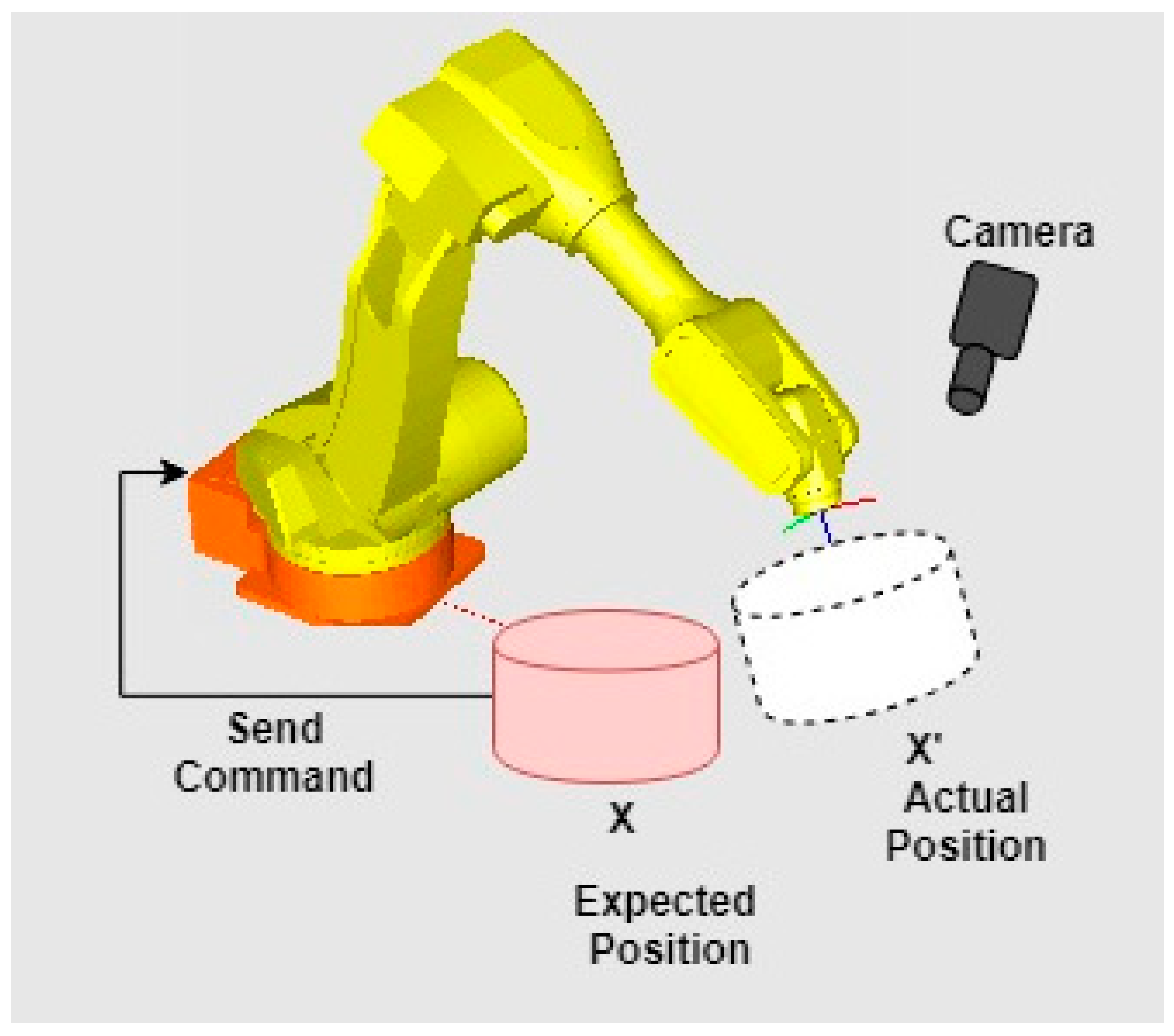
2. Overview of the Problem

The goal of the error compensation approach is to reduce the position error of the robot tool in the real world during the online operation. The added information, usually the real coordinate value of objects, must be precisely determined with respect to the robot coordinate [18]. One can estimate the pose of the object based on its 3D object model known a priori. The pose of the model in the frame (B) is written as
x W B =   [ t W θ W ]   ,
where t and θ denote the position and the orientation of the object from the world coordinate to the robot base coordinate, respectively. Based on the x W B pose, the transformation matrix describing the model frame (W) relative to the base frame (B) can be determined as follows:
T W B =   [ R W B ( θ W ) t W B 0 1 × 3 1 ]   .
However, the robot has its own error, so that the real pose of the object corresponding to the robot coordinate is different compared to the x W B pose. We denote the real pose as x W B . Figure 1 shows that the positions of these two objects differ from the coordinates of the robot.
In order to pick up objects using the robot, the robot moves to a fine search position. The 3D pose of the correct object is then calculated through the sensor and produces the object coordinates. After calculating the pickup posture considering the 3D posture of the object, the trajectory of the robot is modified to reach the expected position x W B .
In a real-life scenario, however, the robot will reach an actual location x W B due to a robot’s error. From a general point of view, there is a full pose corresponding to the pose x W B of an object that allows the controller to control the robot’s reach. The important problem is that in order to get to the expected pose correctly, the controller will have to do an error compensation, and the actual pose of the robot will be moved to the expected pose. To solve this problem, we proposed a method using a neural network and a machine vision to predict a new pose x n e w W B after training the data inside the workspace.
Figure 2 describes the architecture of the proposed error compensation algorithm for the object picking system. It consists of two stages: the initial stage and the robot operation stage. The first stage includes the pre-error compensation and error compensation operation. In the pre-error compensation, the operator has to register the reference pattern in the workspace; calibrate the camera in order to detect the 3D pose of the pattern as shown in Block 1. Next, the reference pattern will be detected in the error compensation operation; hand-eye calibration work is implemented to build up the coordinate relationship between camera and robot frames, and the position of the robot will be estimated in this operation based on the neural network as shown in Block 2. Finally, the whole process of object picking is described in the robot operation stage, which includes the go-to-fine-search-position to pick-object as shown in Block 3. The main technical functions of the proposed robot error compensation are training the workspace for the robot using the indirect calibration approach.

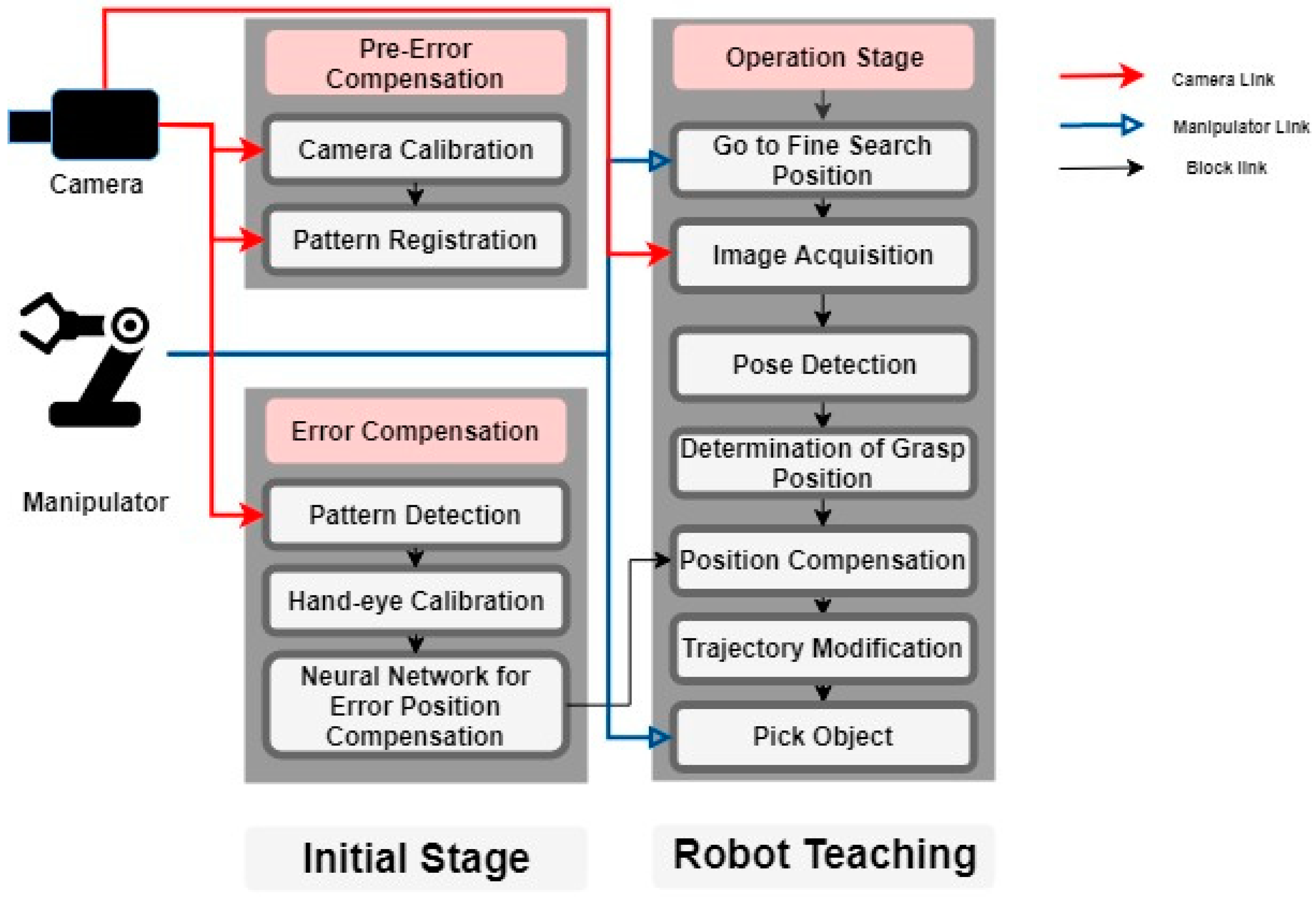
3. Proposed Error Compensation Method

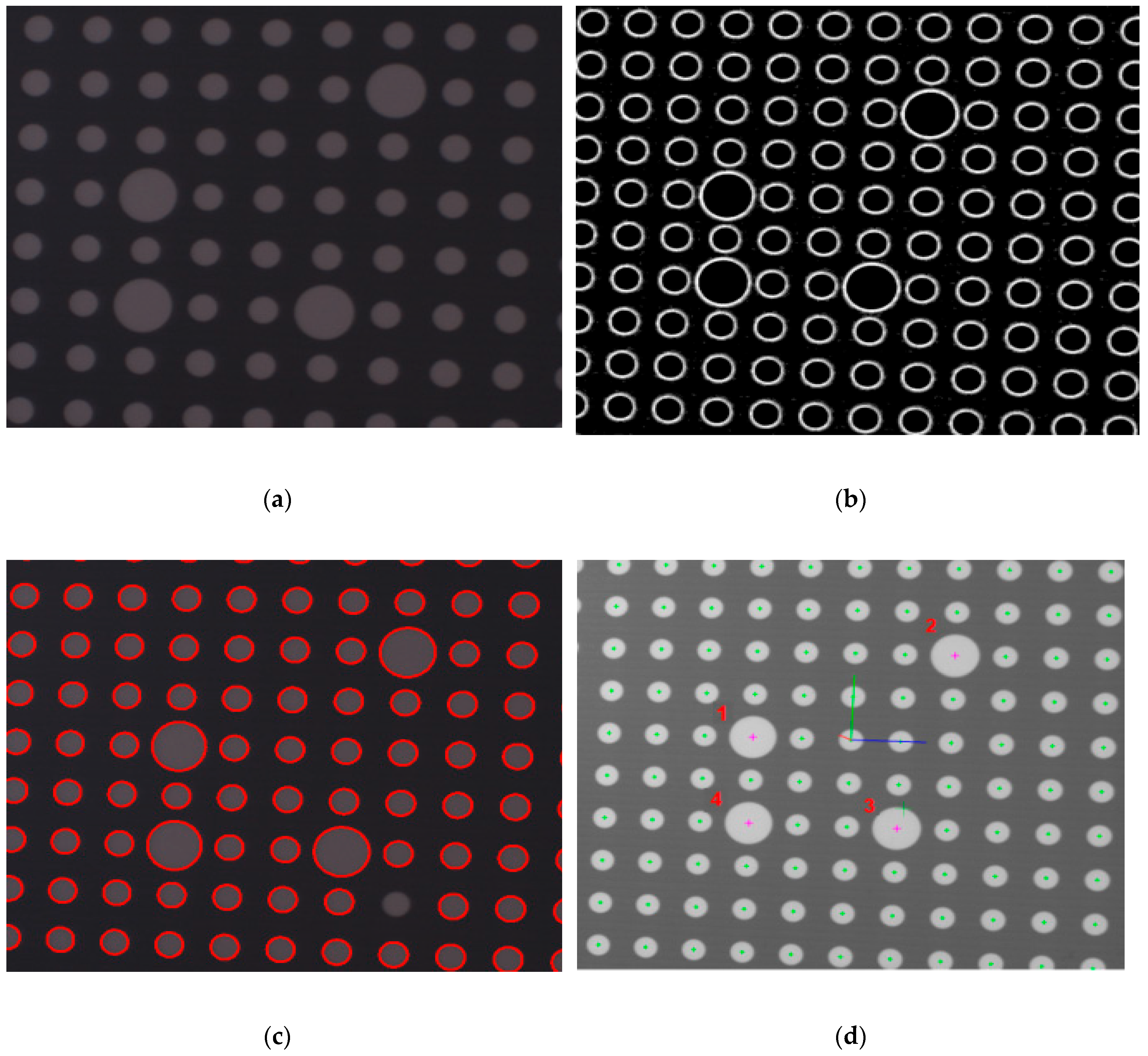
3.1. Pattern Detection and Pose Estimation

In this study, the world coordinate system is located on the pattern board, which is the calibrated workspace for the robot. For simple detection and pose estimation of the pattern board, we designed a specific pattern image as seen in Figure 3a. The circles on the pattern board are numbered as seen in Figure 3d, four bigger circles. The pattern board consists of the key feature made of four big circles, which are used to create the workspace coordinate, and the rest of the circles with smaller size are used for the pose estimation. The operation of the pre-compensation system is divided into two stages: the pattern detection and pose estimation. For pattern image detection we moved the robot to the pattern board, then the hole geometry was extracted from the image. In the pose estimation stage, the Perspective-n-Point (PnP) method based on the RANSAC-algorithm was used to estimate the coordinate of the pattern corresponding to the camera system.
In the pattern detection stage, we extracted the holes section from image data via the edge detection algorithm as shown in Figure 3b. We applied a Difference-of-Gaussian (DoG) filter to remove noise and improve the geometry shape of the holes. DoG is accomplished by convolving the image with a Gaussian filter at different scales. As a result, key-points were extracted from multiple scales, based on the maximum/minimum value of DoG:
D ( x , y , σ ) = ( G ( x , y , k σ ) G ( x , y , σ ) ) I ( x , y )   ,
where G ( x , y , σ ) =   1 2 π σ 2 e ( x 2 + y 2 ) / 2 σ 2 .
In order to increase the reliability of pattern detection, the ellipse fitting techniques were additionally applied for circle detection as shown in Figure 3c. The ellipse-fitting algorithm is a common task in machine vision to estimate the centers and radius of the circle. Let denote a set of 2D data points P =   { x i } i = 1 n ,   w h e r e   x i = ( x i , y i ) , a family of curves C(a) parameterized by the vector a, and the distance metric δ ( C ( a ) , x ) which measures the distance from a point x to the curve C ( a ) . The problem is to find the value a m i n for which the error function ϵ 2 ( a ) =   i = 1 n δ ( C ( a ) , x i ) attains its global minimum. Hence, the curve best fits the data. In this study, the fitting algorithm based on the “approximate mean square distance” metric [19], minimizes the unusual objective function,
ϵ 2 ( a ) =   i = 1 n F ( a , x i ) 2 i = 1 n x F ( a , x i ) 2 = D a 2 D x a 2 + D y a 2   ,
where the matrices D x and D y are the partial derivatives of D with respect to x and y.
Based on the detection stage, key-points localization is suitably implemented using a pose estimation algorithm. To estimate the pose of the pattern, many approaches have been proposed in the literature. For this work, we applied the RANSAC algorithm to estimate the pose. RANSAC is an iterative method proposed to solve the PnP problem [20]. Since then, it has been applied to many machine vision areas such as PnP, visual SLAM, homographic estimation, fundamental or essential matrix estimation, etc. Let assume we have a set of pairs of matched 2D-3D points (corresponding): ( x i ,   X i W ) , as shown in Figure 3d, four major feature points are used to define the workspace coordinate. The final solution is the transformation matrix T W C that transforms from the workspace coordinate to camera coordinate.
Since we applied robust image processing algorithms such as pattern detection and ellipse fitting to increase the performance of 3D position and orientation, the proposed system becomes more reliable on data preparation for the neural network used to compensate the error position.

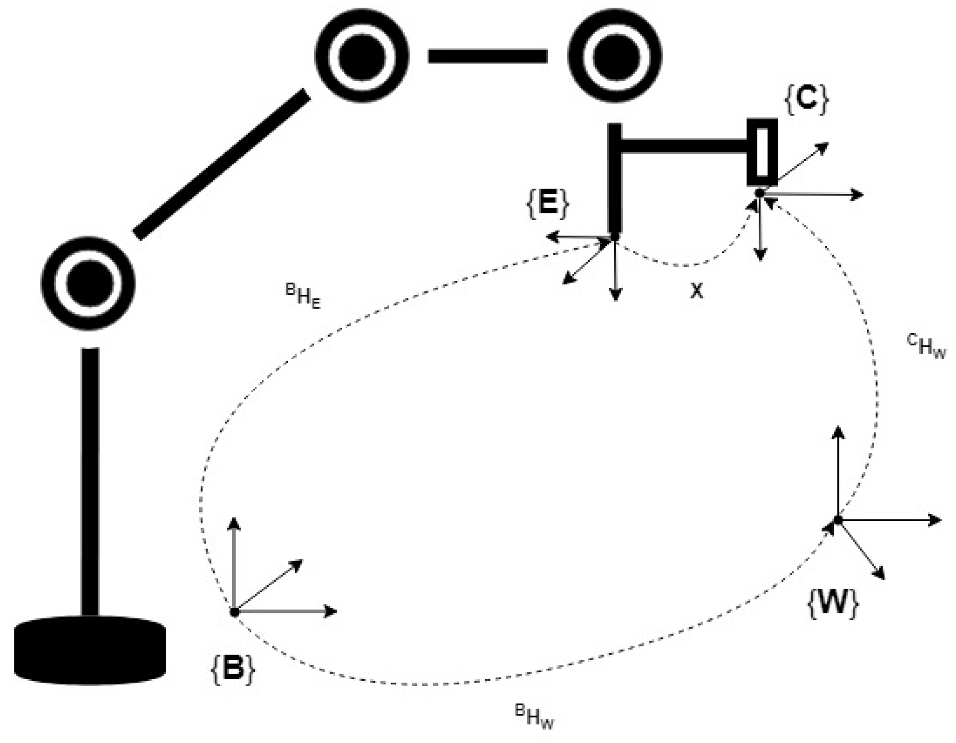
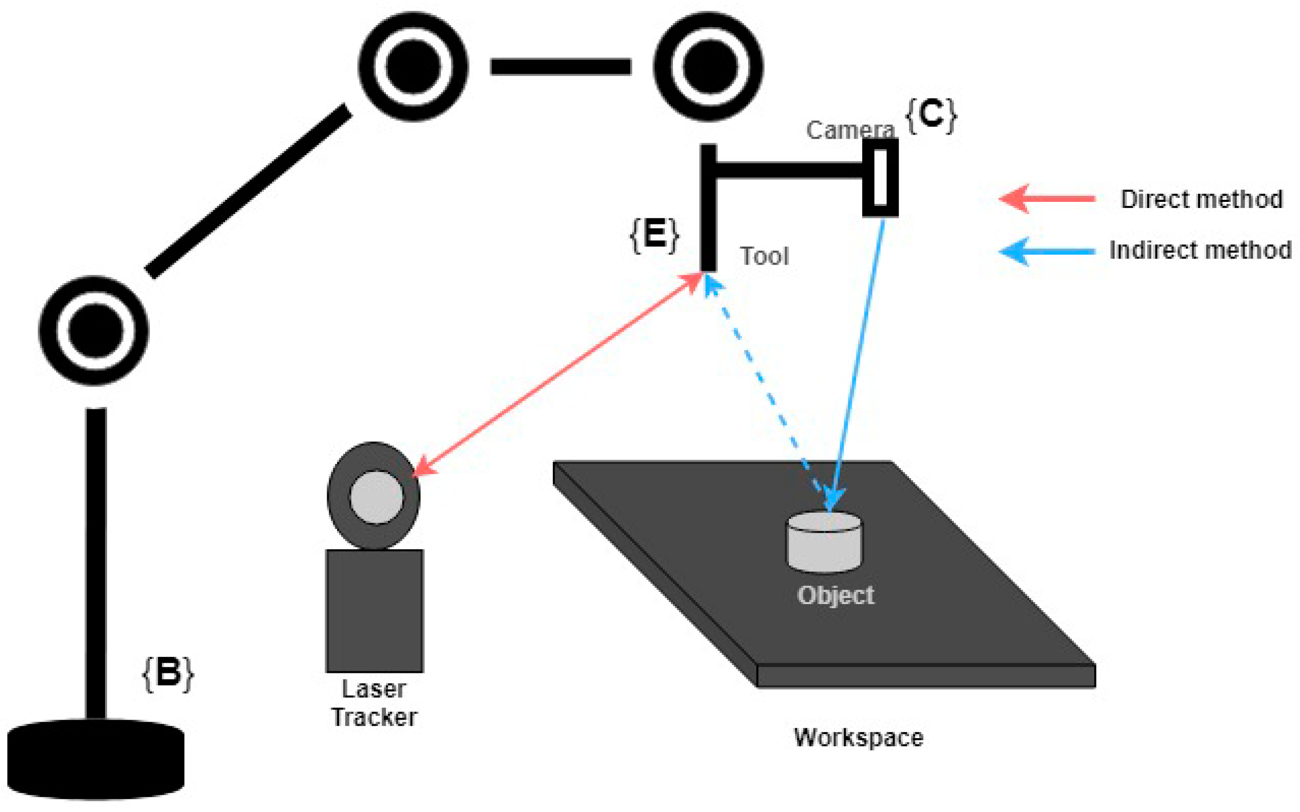
3.2. The Hand-Eye Calibration

The initial vision-based robot involved determining the coordinate relationship between the robot coordinate and the sensor coordinate [21,22]. Common setup of the sensor can be located at a fixed position or can be mounted on the tool of the robot according to a specific application. In this work, the sensor was attached to the tool of the robot for a better field of view in the workspace. The setup of the sensor was fixed on that position during the calibration. If there was any rearrangement about the setting, the calibration was implemented again.
Figure 4 represents the coordinate frames used to perform the hand-eye calibration in this paper, where (B), (E), (C) and (W) are the coordinates of the robot base, the robot, the camera, and the world, respectively. The relationship between each coordinate can be described by a homogenous transformation matrix.
In the literature, several approaches have been published to solve the hand-eye calibration; the problem yields a homogeneous matrix equation of the A X = X B form as the following:
r a r x = r x r b   ,
( r a i 3 ) t x = r x t b t a   ,
where i 3 is 3 × 3 unit matrix r a , r b SO 3 are rotation matrices corresponding to the robot and camera transformation, respectively. r x   S O 3   , t x   R 3 are the rotation matrix and translation matrix, respectively, which denotes X. The linear optimization method is a common solution to solve this equation based on the assumption that A, B satisfy the rigid transformation or their rotation angles in Equation (5) are equal. However, in most cases, their A, B, and X might not satisfy rigid transformation. A direct solution based on the iterative computation with Jacobian optimization is proposed by Jianfei et al. [23]. Given multiple pairs, ( A i ,   B i )   f o r   i = 1 , , n , where i represents the sequence number of the equation   A X = X B . The problem of hand-eye can be stated using the properties of Kronecker product ( ), the Equations (5) and (6) can be written as:
F ( i ) = ( r a ( i ) i 3 i 3 r b t ( i ) ) v e c ( r X )   ,
G ( i ) = ( r a ( i ) i 3 ) t a i t X t b i +   t a i   ,
where v e c is an operation, which stretches a matrix as the row’s direction, v e c ( R X ) R 9 is the vector obtained by stacking the columns of t X , and F ( i ) ,   G ( i ) are the vectors of ( 9 × 1 )   and   ( 3 × 1 ) separately. Find the rotation θ m i n R 3 and the translation t m i n R 3 for which the error function L ( θ ,   t ) = min i [ F ( i ) 2 +   G ( i ) 2 ] attains its global minimum, where L ( θ ,   t ) is the objective function of optimization for solving the hand-eye problem. Let J ( i ) be the Jacobian formula for the object function, H =   [ F ( i ) , G ( i ) , , F ( n ) , G ( n ) ] T can be represented of multi-equations such as Equations (7) and (8). Then the interactive formula for optimization is given as:
J Δ X =   H   ,
X n + 1 =   X n + Δ X   .
The transformation X( θ , t ) is then the solution that best fits the multiple pairs ( A i ,   B i )   f o r   i = 1 , , n . A linear solution can be found using singular value decomposition (SVD) or using a pseudo-inverse.
After solving the hand-eye problem, the object position in the world coordinate corresponding to the robot coordinate can be described as follows:
H W B =   H E B X H W C   ,
H i B =   H W B P i W   ,
where X is obtained from the work above, H E B is provided by the robot controller, H W C is calculated by the pattern detected from the camera, and P i W is the 3D position of the object in world coordinate.

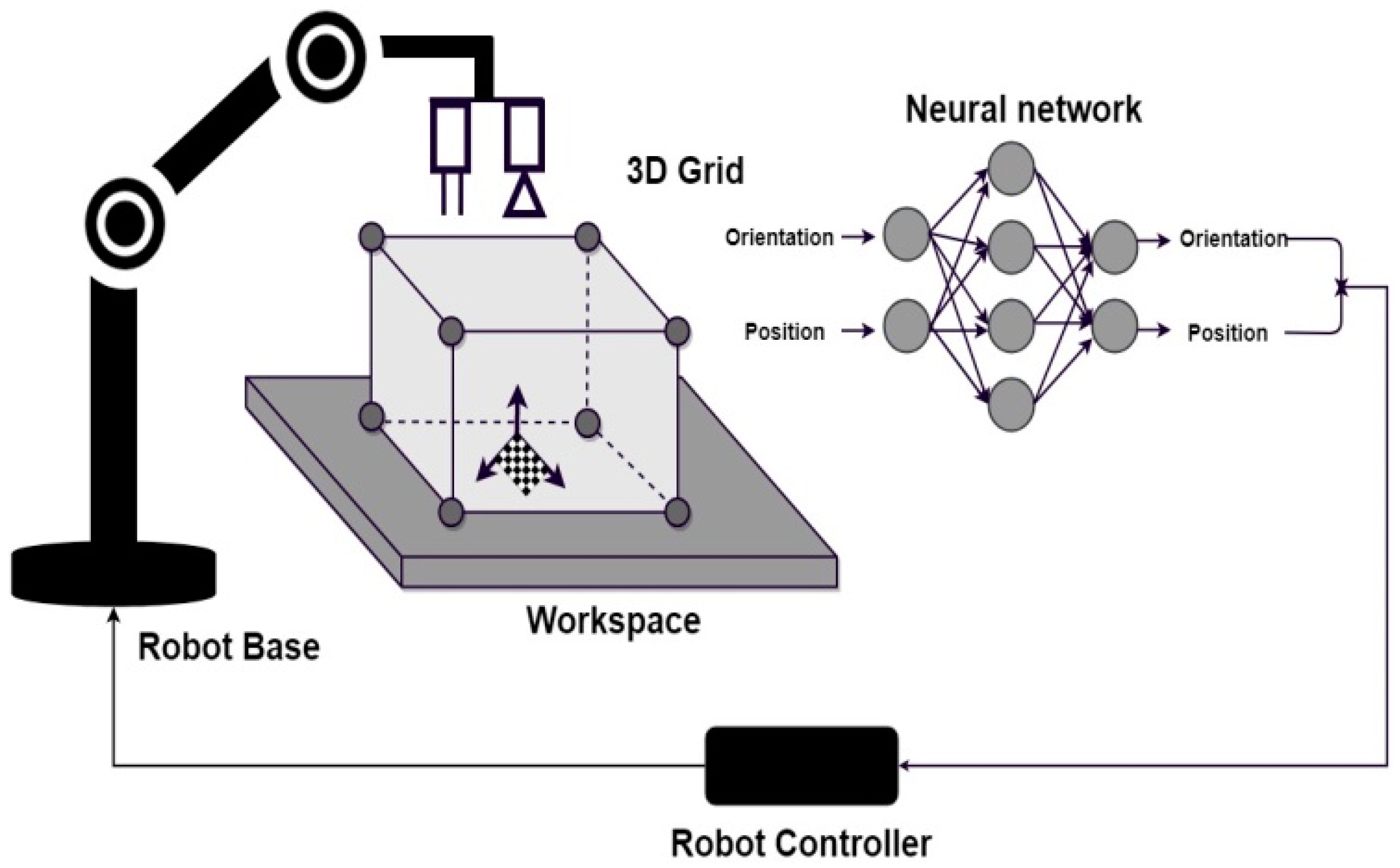
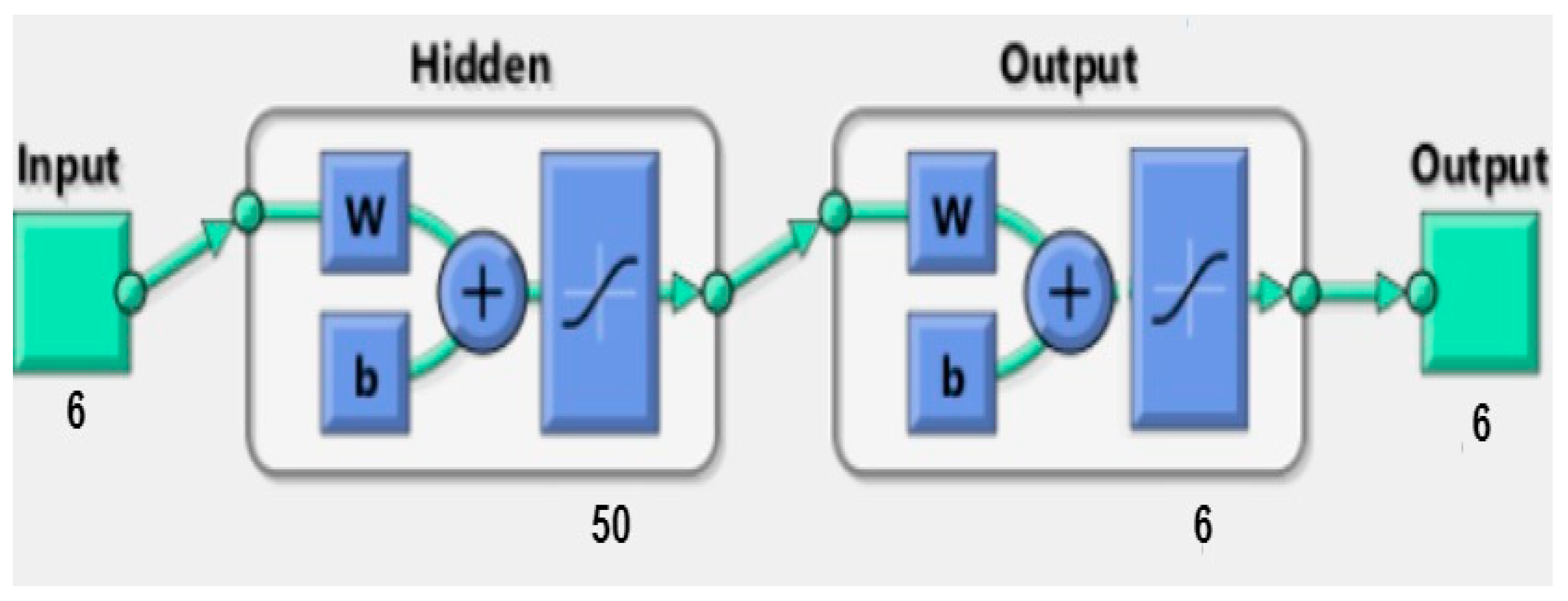
3.3. Feature Training Using Neural Network

A non-parametric kinematics calibration is an approach using intelligent algorithms to reduce the position error without modifying robot parameters [9]. Its advantage is that the position is compensated directly, by which the calibration process can be simplified. Several approaches to error compensation without robot parameter modification are introduced in the literature [24,25]. The real position of the robot can be tracked by using external devices such as a laser tracker, stereo vision, etc. Then, the non-linear approach is used to estimate the error between the actual position and the real position to minimize the error of the robot.
In this paper, we proposed an error compensation method based on advanced machine-vision algorithms and neural network to guide the robot to pick the object. Figure 5 shows the difference between the direct and the indirect approach presented in this paper. When applying the indirect approach, the robot’s end-effector is set to be interpolated, assuming that the coordinate conversion value from the measuring object to the camera coordinate system is obtained accurately. The transformation from the camera coordinate to the root always has a constant value. In addition, the real position of the end-effector and commanded position P a E B from the robot controller is different, so the actual position of the robot controller in the world coordinate frame is defined as:
P a E B = H W B H C W X 1   ,
where X ,   H W B   S E ( 3 ) are obtained from the above, and H C W   S E ( 3 ) is calculated from the camera. To collect information from the workspace, the robot moves to all defined 3D grids to obtain images from the camera to determine the position of the object, where the 3D grid is the workspace where the robot will be trained during the error-compensation stage; finally, the actual position of the robot is calculated by the controller and stored in memory. This data is used for training purposes. Figure 6 shows our proposed method.
The next step is to perform training using measured data. In this paper, we applied a neural network to estimate the actual location of the robot. Neural networks are currently the state of the art method in machine learning [26].
In our experiment, we used a three-layer feedforward neural network to classify different types of defects. Let V = ( V 1 T , V 2 T , , V m T ) T be the weight matrix connecting the input and the hidden layers, where V j = ( V j 1 , , V j n ) for j = 1, 2, …,m. Let W = ( W 1 T , W 2 T , , W p T ) T be the weight matrix between the hidden and the output layers, where W k = ( W k 1 ,   W k 2 , , W k m ) for k = 1, 2,…, p. Given input x =   ( x 1 ,   , x n ) T   R n , and the final output vector o = ( o 1 ,   , o p ) T   R p is given:
o k = f ( W k . y   b k ) = f ( j = 1 m W k j y j b k ) , k = 1 ,   , p .
where { b k } k = 1 p is the biases from hidden to output layers, and y =   ( y 1 ,   , y n ) T   R m is the output of the hidden layer. The distance error is measured based on mean square error, defined as
E ( W , V ) =   1 2 h = 1 H || z h o h || 2   ,
where z n =   ( z 1 ,   , z n ) T   R n is the desired output from the dataset. The update rules based on gradient descent for the weight vector are
W kj ( l + 1 ) =   W kj ( l ) +   η δ E ( W ( l ) , V ( l ) ) δ W kj ,
V kj ( l + 1 ) =   V kj ( l ) +   η δ E ( W ( l ) , V ( l ) ) δ V kj .
where l = 0, 1, 2, …; k = 1, 2, …, p; j = 1, 2, …, m; and i = 1, 2, …, n.

4. Simulation for Robot Model

To improve errors based on the direct approach, the simulation was performed based on PUMA robot parameters before and after compensation using a neural network. For the comparison, two robot models were created: the nominal model and the error model. All DH parameters of the error model added to the nominal model with uniformly distributed noise. Let ε l e n g t h and ε a n g u l a r be the length error magnitude (mm) and angular error offset (deg). The noises added to the nominal model parameters with length error Δ ε l e n g t h (mm) and angular error Δ ε a n g u l a r (deg) are given as:
Δ ε l e n g t h = G ( x l , σ l )   ε l e n g t h   ,
Δ ε a n g u l a r = G ( x a , σ a )   ε a n g u l a r   ,
where G ( x , σ ) =   1 2 π σ 2 e x 2 / 2 σ 2 ,   x , σ are the mean and standard deviation. The geometric errors in the robot-link could be written as Δ a i ,   Δ α i ,   Δ d i ,   Δ θ i while the original parameters of the robot-link i t h were denoted as a i ,   α i ,   d i ,    θ i . The parameters of error model are as following: a i r =   a i + Δ a i   ( m m ) , α i r =   α i + Δ α i   ( m m ) , d i r =   d i + Δ d i (mm).
Where Δ is the noise determined in Equations (18) and (19). The actual values for two kinematic models are shown in Table 1 and Table 2, respectively. In this simulation, ε l e n g t h = 10   mm , and ε a n g u l a r = 2 d e g .
Firstly, the simulation was based on the neural network combined with the laser tracker system. The simulation describes the use of an artificial neural to estimate the robot’s end-effector where the actual positions of end-effector in the workspace are known. The robot is moved to all 3D grid points, all position errors in the 3D grid are measured and recorded by the laser tracker system, and these position errors are stored in the memory to train the neural network. The simulation results are shown in Figure 7. The errors have been improved after the compensation. However, a direct approach using a laser tracker is not well suited for vision-based robot applications because of the cost-effectiveness of the external measuring device and the elaborate setup for the calibration procedure.
Secondly, to illustrate the validity of the proposed method, this section performs error compensation in the simulation environment of the PUMA 560 robot model. For comparison, two robot models were created the same as above. The data generated in this simulation for solving the hand-eye vision problem and training the neural network is also described in this section.

4.1. Simulation Procedure

The procedure for the simulation process is divided into two phases. In the first phase, data is collected from both models. An error compensation assessment is then performed. For the first step, for the hand-eye calibration (AX = XB), real data for the transformation matrix A i was generated by the nominal robot model and data for the transformation matrix B i was generated by the robot error model. Next, in the training for the neural network section, m (m = 686) set of samples were used, and 200 random samples on various positions and orientations in the work coordinate frame were examined for testing. In addition, the distance between the neighboring of each grid points was 28.5 (mm) in all three directions X, Y, and Z, which is an empirical interval for a mid-size calibration space. In total, the workspace includes 343 cells ( 7 × 7 × 7   mm 3 ) . At each cell, two different orientations were taken.
In the error compensation stage, a generalized feed-forward neural network is used. This network consists of one hidden layer. As presented in Figure 8, there are 50 neurons in the hidden layer. The desired position and orientation x =   ( x 1 ,   , x 6 ) T   R 6 of the robot’s end-effector is taken as input layer nodes, and the related position/orientation o = ( o 1 ,   , o 6 ) T   R 6 for robot controller is taken as the output layer nodes.

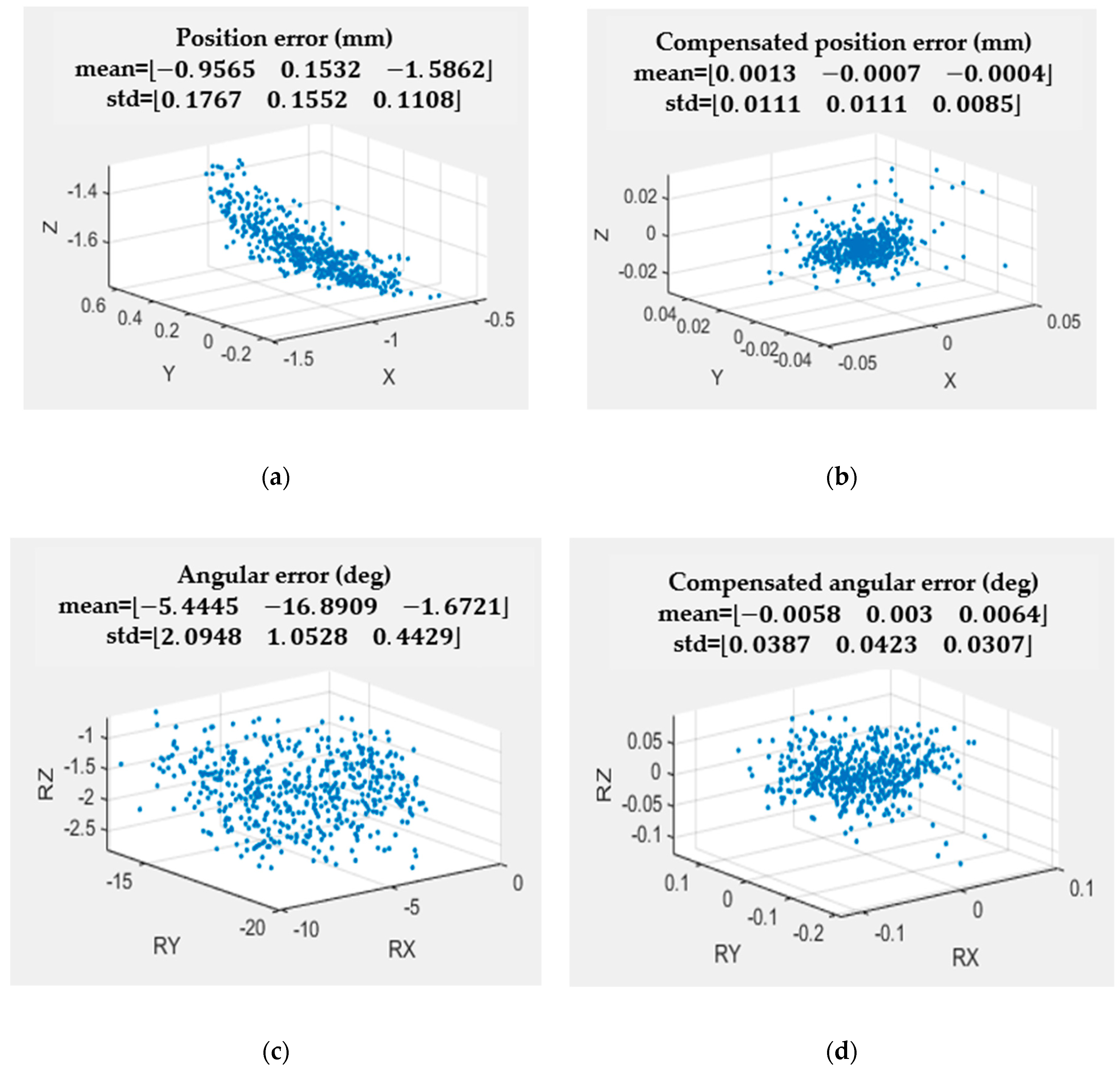
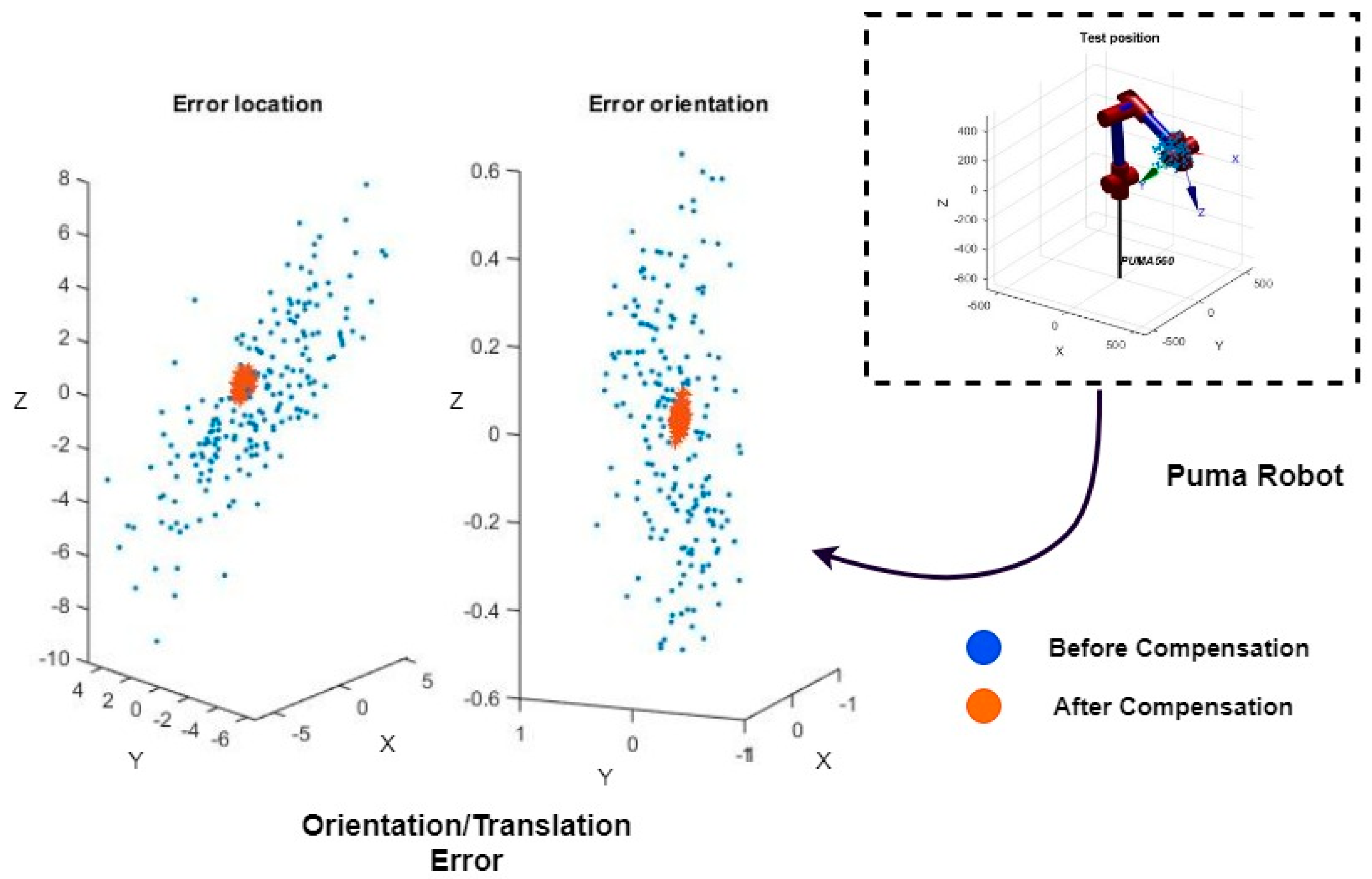
4.2. Simulation Results

After training the neural network, we used 200 test data to evaluate the performance of position/orientation error, and the results are shown in Figure 9.
In Figure 9, the blue area is the result of the robot system before training, while the red area is the result after applying neural network training. The position error t E r r o r = ( t x ,   t y , t z ) T   R 3 and θ E r r o r = ( θ x ,   θ y , θ z ) T   R 3 are defined as follows:
t E r r o r =   t e s t i m a t e d t r e a l   ,
θ E r r o r =   θ e s t i m a t e d θ r e a l   .
As you can see in Figure 9, the errors have been greatly reduced when using the method proposed in this paper. In addition, you can see that applying the neural network to the indirect compensation approach significantly reduces the mean and standard deviation of error.
Table 3 shows that the mean error decreased significantly when the error was compensated using the neural network compared to when the error was not compensated. The mean position errors after compensation are e t x =   −0.0295 (mm), e t y =   −0.0079 (mm), and e t z =   −0.0496 (mm), for which the errors are reduced by 98% on average. As shown in Table 4, the standard deviation for position/orientation error was greatly reduced: e t x =   0.3583 (mm), e t y =   0.5101 (mm), and e t z =   0.03634 (mm), approximately 94% of error reduction on average.

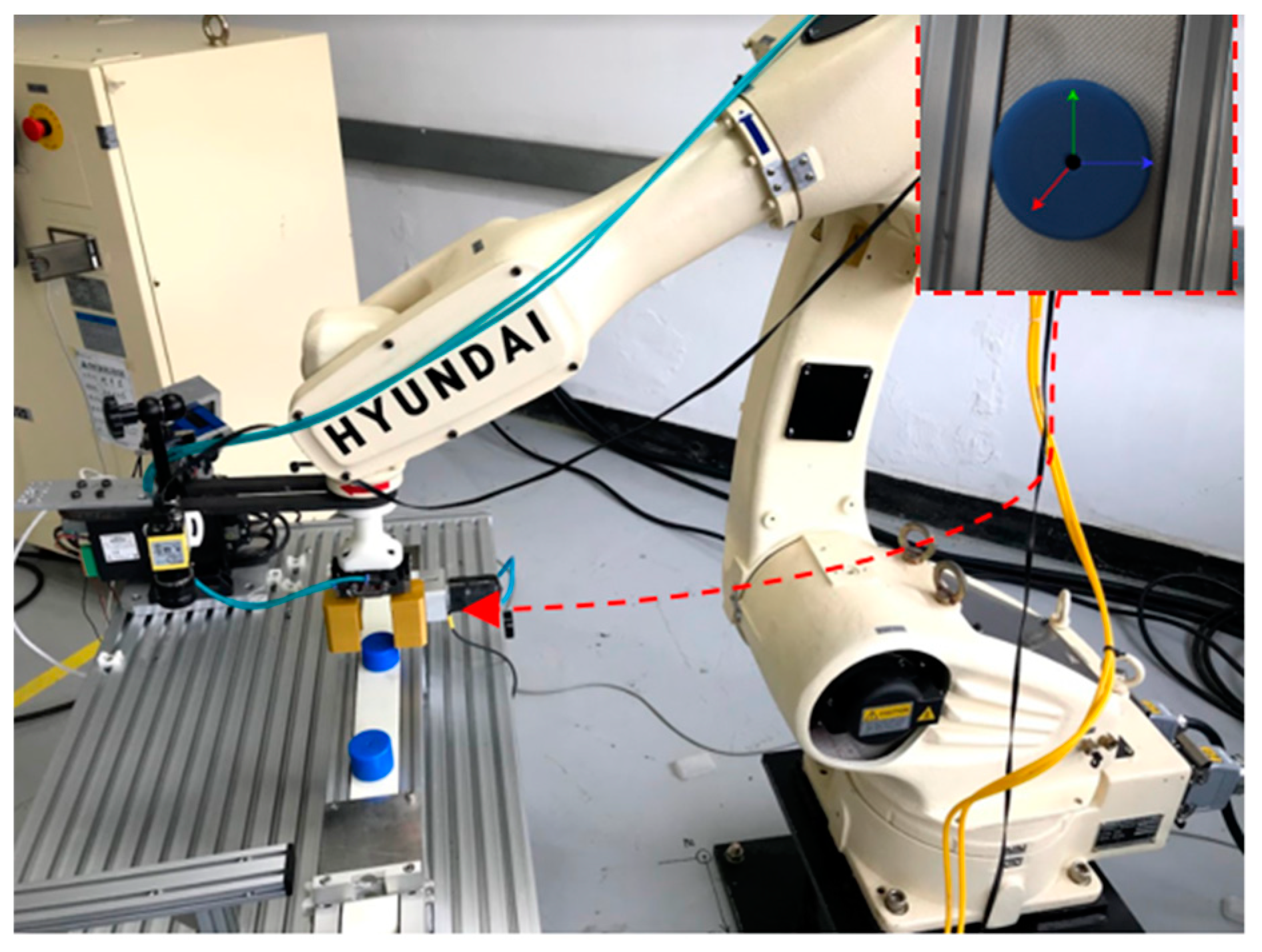
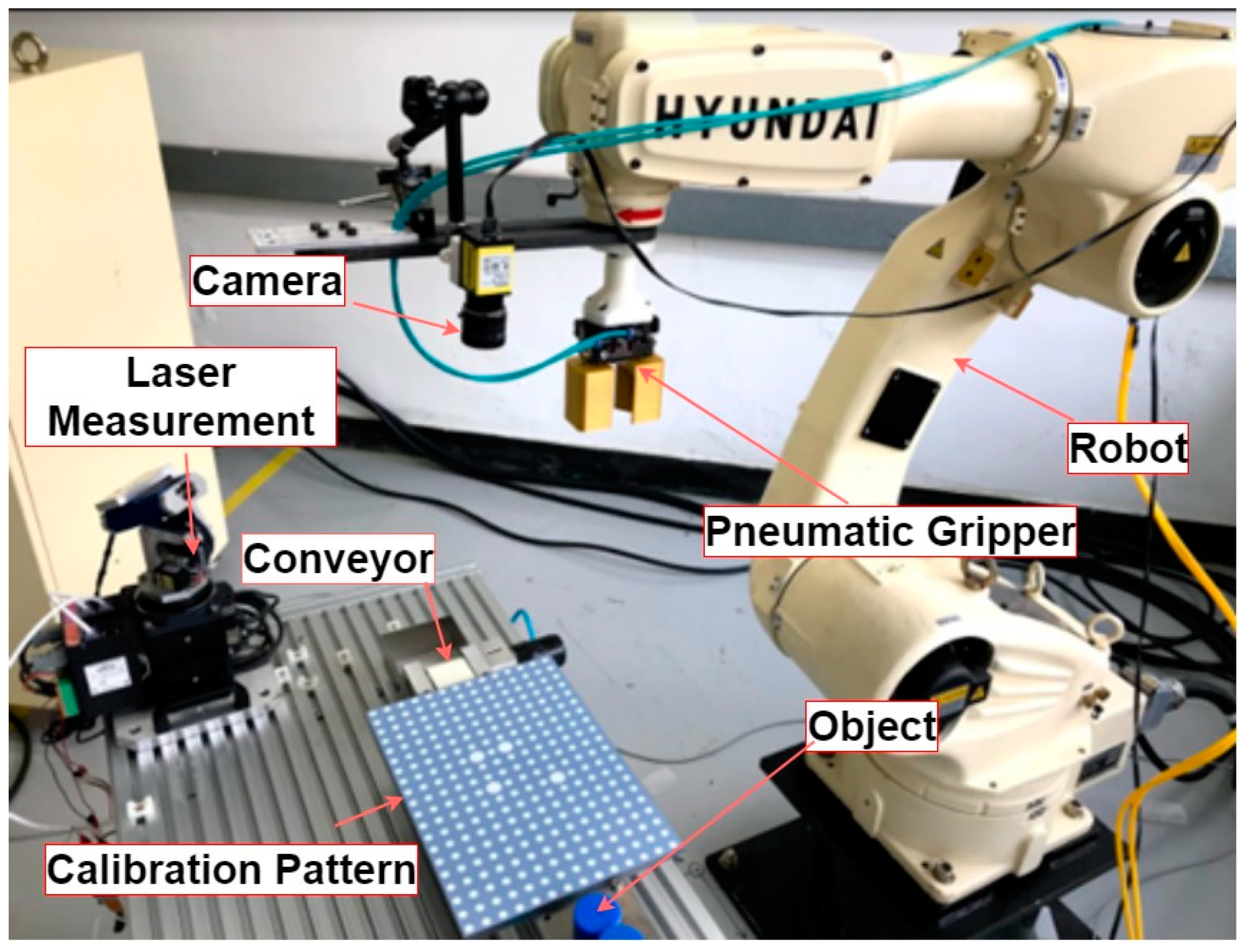
5. Experimental Results

We used a Hyundai Hi5 (HA006 model) 6-axis industrial robot to conduct the experiment. A high-resolution (12 Mp) baser camera with a focal length of 8 mm was attached to the end effector of the robot. In addition, a pneumatic gripper was attached to the robot’s end-effector to enable the robot to grasp objects. The overall robot system is shown in Figure 10.

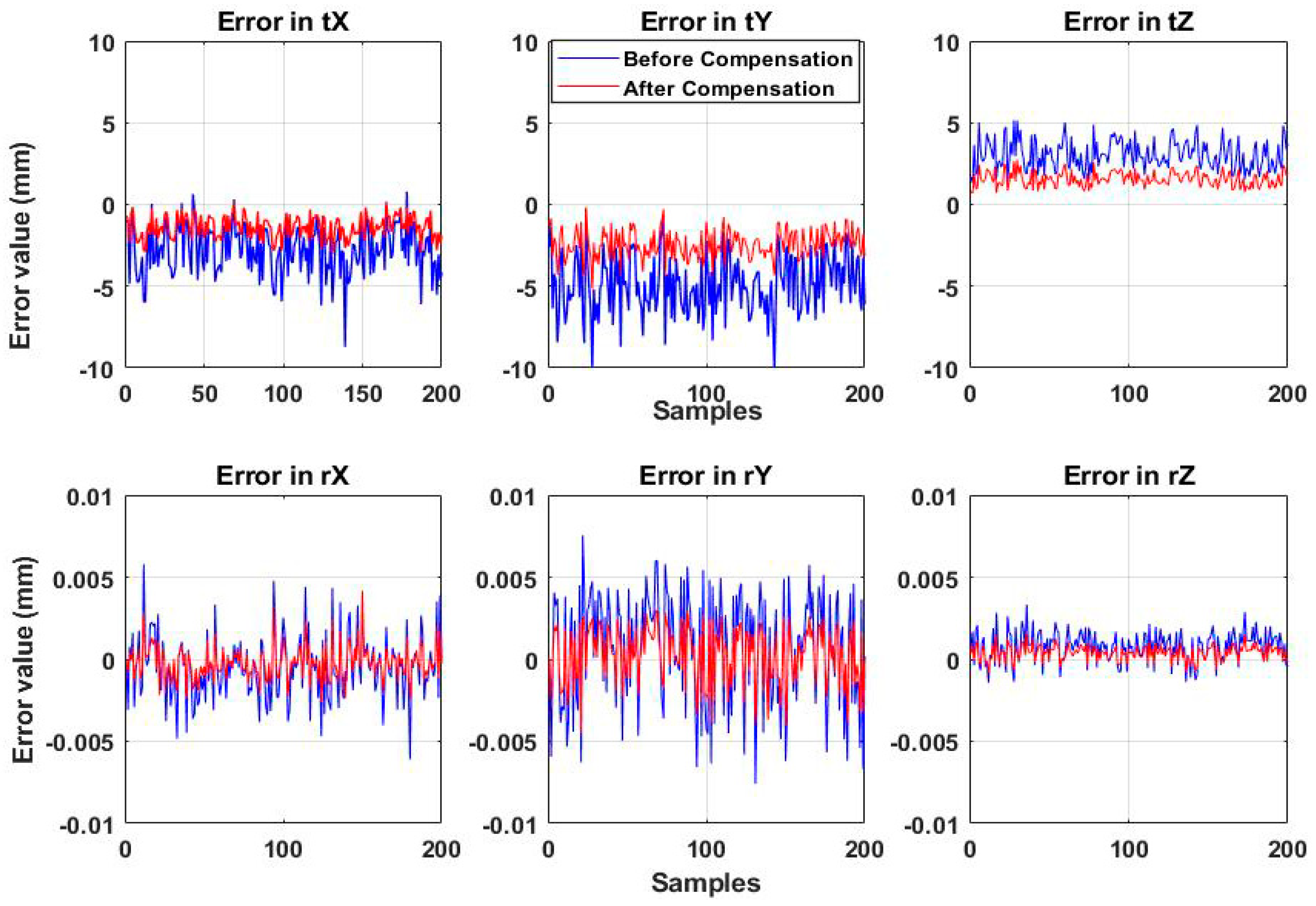
5.1. Experiments on Position/Orientation Error

To evaluate the performance of the proposed system, we compared the calculated amount of movement of the robot to the actual amount of movement. The amount of robot movement can be easily calculated using Equation (13). In this error evaluation process, 686 data samples were used for neural network training, and 200 data samples were used for testing the neural network. The test results are shown in Figure 11. Although the actual results are not as good as the results from the simulation environment, they have reduced the position/orientation error sufficiently. The after compensation value of mean error-position in each direction as shown in Table 5 are e t x =   −1.3897 (mm), e t y = −2.4289 (mm), and e t z =   1.554 (mm), for which the error was reduced by 50.3% on average.
In Table 6, the standard deviation for position/orientation errors after compensation are greatly reduced: e t x =   0.6998 (mm), e t y =   0.8826 (mm), and e t z =   0.4484 (mm), approximately 69% of error reduction on average. The proposed method showed good performance as a result of the experiment. In Figure 11, the after-compensation error (red line) is smaller and smoother than the before compensation error (blue line) when applying the error compensation technique. This illustrates that the absolute position error of the robot’s end-effector is improved. Considering the calculated data from the simulation and experiment as shown in Table 3, Table 4, Table 5 and Table 6, respectively, the compensation improvement of the experimental cases is smaller than the result of the simulation cases. The main reason is that it is really difficult in the real experiment to consider all factors that lead to the absolute position error of the robot’s end-effector such as tolerances, eccentricities, wear-out, payload, temperature and insufficient knowledge of model parameters for the transformation between robot poses, etc. [5]. However, our algorithm did reduce the absolute position error in real experiments by 50.3%, which can verify the proposed compensation algorithm to be utilized successfully in the real application.
Comparing the compensation performance the other works, Liu et al. [27] proposed an improved method for the pose accuracy of the robot manipulator by using a multiple-sensor combination measuring system (MCMS). In their experiments, the pose accuracy of the manipulator is improved by 67.3%, to 3.379 mm on average with the Kamal filter (KF) and by 38.2%, to 1.286 mm on average with multi-sensor optimal information fusion algorithm (MOIFA). Yauheni et al. [2] proposed a method of robot end-effector pose accuracy improving using joint error mutual compensation, the improved value of positioning accuracy for the robot end-effector from 2% to two times, to Δ L = 2.39 mm on average. Hence, it can be concluded that our proposed method gives a better performance on the whole, both in terms of the error reduction ratio and the absolute position error, which is a quite acceptable error in robot application in the real field.

5.2. The Qualitative Experiments Results

To verify the validity of the error compensation method proposed in this paper, an object-picking task was performed using the robot used in the experiment. The procedure for the object picking task is described in Figure 2. Using C#, control software was developed and Raspberry board was used for communication with the robot. Communication was carried out using the RS-232 standard. First, the robot was moved to the fine search position in the field-of-view area of the camera. Then, the camera was used to calculate the 3D pose of an object and then combined with the information of the hand-eye calibration. Then, the position and the normal vector of the object was calculated. Next, the position/orientation value of the end effector was estimated using a neural network. Finally, the robot’s trajectory was modified, and the robot’s gripper reached the target object. The photo of the robot’s picking task is shown in Figure 12 and Figure 13.
The results of the experiment confirmed that the proposed method reduced the absolute position error in the workspace with 200 random positions by 50.3% on average, which is sufficiently applicable to the object-picking task. We are confident that applying the method proposed in this paper to robots will also allow for tasks requiring higher accuracy.

6. Conclusion

In this paper, the proposed indirect calibration approach is proved to compensate for the absolute position/orientation error of a six-axis industrial robot throughout the simulations and experiments. In particular, experiments with an object picking task using a robot and camera were also conducted to substantively demonstrate the validity of the proposed algorithm. The position/orientation of the robot’s end-effector is compensated without modifying the robot’s parameters. The proposed method is based on a machine vision algorithm combined with a neural network. Using the robot’s end-effector as an input for a neural network, and the camera attached on the end-effector to observe the object, we successfully improved the absolute position error of the robot in the workspace. According to the simulation results, location errors decreased by 98%. The average value of the absolute position error was 0.029 mm. Actual results showed that the absolute position error was reduced to 50.3% and the average value of the absolute position error was 1.79 mm, which is a quite acceptable error in robot application in the real field [5,6,7]. In conclusion, the proposed method is well suited for simply deploying the robot visual system in different manufacturing environments because no external measuring equipment or complicated setup is required in the error compensation and makes the calibration procedure more convenient to implement. We believe that the method proposed in this paper can also be applied to robot tasks requiring a high degree of accuracy and replace the existing error-compensating methods.

Author Contributions

All authors read and approved the manuscript. Conceptualization, C.-T.C.; methodology, C.-T.C. and V.-P.D.; Software, C.-T.C. and V.-P.D.; validation, C.-T.C. and B.-R.L.; format analysis, C.-T.C. and B.-R.L.; investigation, C.-T.C.; resource, C.-T.C.; Writing—Original Draft preparation, C.-T.C.; Writing—Review and Editing, B.-R.L.; visualization, C.-T.C.; supervision, B.-R.L.

Acknowledgments

This work was supported by the 2019 Research Fund of University of Ulsan.

Conflicts of Interest

The authors declare no conflict of interest

References

  1. Oh, J.-K.; Lee, S.; Lee, C.-H. Stereo vision based automation for a bin-picking solution. Int. J. Control Autom. Syst. 2012, 10, 362–373. [Google Scholar] [CrossRef]
  2. Yauheni, V.; Jerzy, K. Application of joint error mutual compensation for robot end-effector pose accuracy improvement. J. Intell. Robot. Syst. Theory Appl. 2003, 36, 315–329. [Google Scholar]
  3. Darmanin, R.N.; Bugeja, M.K. A review on multi-robot systems categorised by application domain. In Proceedings of the 2017 25th Mediterranean Conference on Control and Automation (MED), Valletta, Malta, 4–6 July 2017; pp. 701–706. [Google Scholar]
  4. Njaastad, E.B.; Egeland, O. Automatic Touch-Up of Welding Paths Using 3D Vision. IFAC-PapersOnLine 2016, 49, 73–78. [Google Scholar] [CrossRef]
  5. Pérez, L.; Rodríguez, Í.; Rodríguez, N.; Usamentiaga, R.; García, D. Robot Guidance Using Machine Vision Techniques in Industrial Environments: A Comparative Review. Sensors 2016, 16, 335. [Google Scholar] [CrossRef] [PubMed]
  6. Labudzki, R.; Legutko, S. Applications of Machine Vision. Manuf. Ind. Eng. 2011, 2, 27–29. [Google Scholar]
  7. Wöhler, C. 3D Computer Vision: Efficient Methods and Applications; Springer: Dortmund, Germany, 2009. [Google Scholar]
  8. Roth, Z.; Mooring, B.; Ravani, B. An overview of robot calibration. IEEE J. Robot. Autom. 1987, 3, 377–385. [Google Scholar] [CrossRef]
  9. Xuan, J.Q.; Xu, S.H. Review on kinematics calibration technology of serial robots. Int. J. Precis. Eng. Manuf. 2014, 15, 1759–1774. [Google Scholar] [CrossRef]
  10. Nubiola, A.; Bonev, I.A. Absolute calibration of an ABB IRB 1600 robot using a laser tracker. Robot. Comput. Integr. Manuf. 2013, 29, 236–245. [Google Scholar] [CrossRef]
  11. Nubiola, A.; Bonev, I.A. Absolute robot calibration with a single telescoping ballbar. Precis. Eng. 2014, 38, 472–480. [Google Scholar] [CrossRef]
  12. Kubota, T.; Aiyama, Y. Calibration of relative position between manipulator and work by Point-to-face touching method. In Proceedings of the 2009 IEEE International Symposium on Assembly and Manufacturing, Suwon, Korea, 17–20 November 2009; pp. 286–291. [Google Scholar]
  13. Bai, Y.; Zhuang, H.; Roth, Z.S. Experiment study of PUMA robot calibration using a laser tracking system. In Proceedings of the 2003 IEEE International Workshop on Soft Computing in Industrial Applications, Binghamton, NY, USA, 25 June 2003; pp. 139–144. [Google Scholar]
  14. Ha, I.-C. Kinematic parameter calibration method for industrial robot manipulator using the relative position. J. Mech. Sci. Technol. 2008, 22, 1084–1090. [Google Scholar] [CrossRef]
  15. Meng, Y.; Zhuang, H. Autonomous robot calibration using vision technology. Robot. Comput. Integr. Manuf. 2007, 23, 436–446. [Google Scholar] [CrossRef]
  16. Gong, C.; Yuan, J.; Ni, J. A Self-Calibration Method for Robotic Measurement System. J. Manuf. Sci. Eng. 2000, 122, 174–181. [Google Scholar] [CrossRef]
  17. Yin, S.; Ren, Y.; Zhu, J.; Yang, S.; Ye, S. A Vision-Based Self-Calibration Method for Robotic Visual Inspection Systems. Sensors 2013, 13, 16565–16582. [Google Scholar] [CrossRef] [PubMed]
  18. Chang, W.-C.; Wu, C.-H. Eye-in-hand vision-based robotic bin-picking with active laser projection. Int. J. Adv. Manuf. Technol. 2016, 85, 2873–2885. [Google Scholar] [CrossRef]
  19. Fitzgibbon, A.; Fisher, R. A Buyer’s Guide to Conic Fitting. In Proceedings of the British Machine Vision Conference 1995; British Machine Vision Association: Durham, UK, 1995; pp. 51.1–51.10. [Google Scholar]
  20. Marchand, E.; Uchiyama, H.; Spindler, F. Pose Estimation for Augmented Reality: A Hands-On Survey. IEEE Trans. Vis. Comput. Graph. 2016, 22, 2633–2651. [Google Scholar] [CrossRef] [PubMed]
  21. Park, F.C.; Martin, B.J. Robot sensor calibration: Solving AX=XB on the Euclidean group. IEEE Trans. Robot. Autom. 1994, 10, 717–721. [Google Scholar] [CrossRef]
  22. Strobl, K.H.; Hirzinger, G. Optimal Hand-Eye Calibration. In Proceedings of the 2006 IEEE/RSJ International Conference on Intelligent Robots and Systems, Beijing, China, 9–15 October 2006; pp. 4647–4653. [Google Scholar]
  23. Jianfei, M.; Qing, T.; Ronghua, L. A Direct Linear Solution with Jacobian Optimization to AX=XB for Hand-Eye Calibration. WSEAS Trans. Syst. Control 2010, 5, 509–518. [Google Scholar]
  24. Bai, Y.; Zhuang, H. Modeless robots calibration in 3D workspace with an on-line fuzzy interpolation technique. In Proceedings of the 2004 IEEE International Conference on Systems, Man and Cybernetics (IEEE Cat. No.04CH37583), The Hague, The Netherlands, 10–13 October 2004; Volume 6, pp. 5233–5239. [Google Scholar]
  25. Wang, D.; Bai, Y.; Zhao, J. Robot manipulator calibration using neural network and a camera-based measurement system. Trans. Inst. Meas. Control 2012, 34, 105–121. [Google Scholar] [CrossRef]
  26. Yang, S.; Zhang, C.; Wu, W. Binary output layer of feedforward neural networks for solving multi-class classification problems. arXiv 2018, arXiv:1801.07599. [Google Scholar] [CrossRef]
  27. Liu, B.; Zhang, F.; Qu, X. A Method for Improving the Pose Accuracy of a Robot Manipulator Based on Multi-Sensor Combined Measurement and Data Fusion. Sensors 2015, 15, 7933–7952. [Google Scholar] [CrossRef] [PubMed]
Figure 1. Difference between expected and actual robot position.
Applsci 09 01940 g001
Figure 2. The overall architecture of proposed error compensation algorithm.
Applsci 09 01940 g002
Figure 3. Pattern detection and pose estimation. (a) Original image, (b) edge detection, (c) ellipse fitting, (d) pose detection.
Applsci 09 01940 g003
Figure 4. Coordinates for hand-eye calibration.
Applsci 09 01940 g004
Figure 5. An indirect method for robot calibration.
Applsci 09 01940 g005
Figure 6. Indirect method for robot error-compensation.
Applsci 09 01940 g006
Figure 7. The error compensation results. (a) position error (mm) (b) compensated position error (mm) (c) angular error (deg) (d) compensated angular error (deg).
Applsci 09 01940 g007
Figure 8. Architecture developed for the neural network.
Applsci 09 01940 g008
Figure 9. Position/orientation error in 3D space for simulation.
Applsci 09 01940 g009
Figure 10. Setup for training robot.
Applsci 09 01940 g010
Figure 11. Comparison between before and after compensation in the experiment environment.
Applsci 09 01940 g011
Figure 12. Trajectory that the robot was taught.
Applsci 09 01940 g012
Figure 13. Object picking result.
Applsci 09 01940 g013
Table 1. DH parameters of the nominal model.
Link No. θ i / r a d d i / m m a i / m m α i / r a d
1 θ 1 001.5708
2 θ 2 04320
3 θ 3 15020−1.5708
4 θ 4 43201.5808
5 θ 5 00−1.5708
6 θ 6 000
Table 2. DH parameters of the error model.
Link No. θ i / r a d d i / m m a i / m m α i / r a d
1 θ 1 2.424633.4331.65256
2 θ 2 5.92042433.9660.031139
3 θ 3 150.02320.0033−1.441
4 θ 4 436.2970.3175391.5975
5 θ 5 5.577961.30921−1.4774
6 θ 6 4.176436.275150.1111
Table 3. Mean error of the measurement system position-accuracy.
MeasurementMean Error
Translation/mmRotation/rad
e t x e t y e t z e θ x e θ y e θ z
Before0.9883−1.31732.37430.0008−0.0062−0.0032
After−0.0295−0.0079−0.0496−0.00000.00020.0000
Reduced %97.01%99.4%97.9%100%96.77%100%
Table 4. Standard deviation error.
MeasurementStandard Deviation Error
Translation/mmRotation/rad
e t x e t y e t z e θ x e θ y e θ z
Before12.418210.47638.79840.02020.02150.0171
After0.26320.42560.38810.00060.00060.0006
Reduced %97.88%95.93%95.58%97.02%97.21%96.49%
Table 5. Mean error of the measurement system position accuracy.
MeasurementMean Error
Translation/mmRotation/rad
e t x e t y e t z e θ x e θ y e θ z
Before−2.9269−4.98402.9249−0.00040.00070.0008
After−1.3897−2.42891.5540−0.00020.00040.00045
Reduced %52.52%51.27%46.87%50%42.86%43.75%
Table 6. Standard deviation error.
MeasurementStandard Deviation Error
Translation/mmRotation/rad
e t x e t y e t z e θ x e θ y e θ z
Before2.24612.37261.74130.00190.00360.0010
After0.69980.88260.44840.00100.00180.00055
Reduced %68.84%62.80%74.25%47.37%50%45%

