Enhancing Recommendation Accuracy of Item-Based Collaborative Filtering via Item-Variance Weighting

Abstract

Recommender systems (RS) analyze user rating information and recommend items that may interest users. Item-based collaborative filtering (IBCF) is widely used in RSs. However, traditional IBCF often cannot provide recommendations with good predictive and classification accuracy at the same time because it assigns equal weights to all items when computing similarity and prediction. However, some items are more relevant and should be assigned greater weight. To address this problem, we propose a niche approach to realize item-variance weighting in IBCF in this paper. In the proposed approach, to improve the predictive accuracy, a novel time-related correlation degree is proposed and applied to form time-aware similarity computation, which can estimate the relationship between two items and reduce the weight of the item rated over a long period. Furthermore, a covering-based rating prediction is proposed to increase classification accuracy, which combines the relationship between items and the target user’s preference into the predicted rating scores. Experimental results suggest that the proposed approach outperforms traditional IBCF and other existing work and can provide recommendations with satisfactory predictive and classification accuracy simultaneously.

1. Introduction

Recommender systems (RS) can provide personalized recommendations for various types of users [1,2,3,4]. Thus, such systems are widely used, have significant commercial value and have been studied extensively [5,6,7,8].

RSs rate items that users have not yet purchased and recommend items based on user preferences [9,10]. Consequently, recommendation accuracy directly affects RS service quality and user experience, because it measures how well an RS can predict an exact rating value for a specific item. Generally, RS accuracy metrics include predictive accuracy and classification accuracy [11,12]. Predictive accuracy indicates the average error between predictions and real values. For example, in the MovieLens dataset, a user will give each movie rating stars which represent the user’s reference degree, the predictive accuracy will evaluate how close predictions are to the user’s true number of stars given to each movie. On the other hand, classification accuracy indicates the extent to which the user agrees with the recommendations; it does not attempt to directly measure the ability of an RS to accurately predict ratings [11]. Note that high predictive accuracy of recommendations does not necessarily imply high classification accuracy, vice versa. It is because even if an RS can correctly rank a user’s movie recommendations, it could fail if the predicted rating scores are incorrect.

Collaborative filtering (CF) approaches are often used in RSs because they perform well [13,14,15]. Item-based collaborative filtering (IBCF) assumes that a user will prefer an item if it is similar to past preferences. Recently, IBCF has demonstrated success in both research and practical applications [16,17], for example, Amazon. In traditional IBCF, all items are assigned the same weight when computing similarity and predictions; however, it is widely recognized that some items are more important than others and should be given relatively higher weight. It will result in the traditional IBCF often cannot provide recommendations with satisfactory accuracy. Currently, many approaches have been proposed to improve the recommendation accuracy of IBCF; however, their results indicate that they can enhance predictive accuracy or classification accuracy but not in both [18,19,20,21,22]. Therefore, how to achieve improvements in both predictive and classification accuracy of IBCF is a difficult problem faced by researchers.

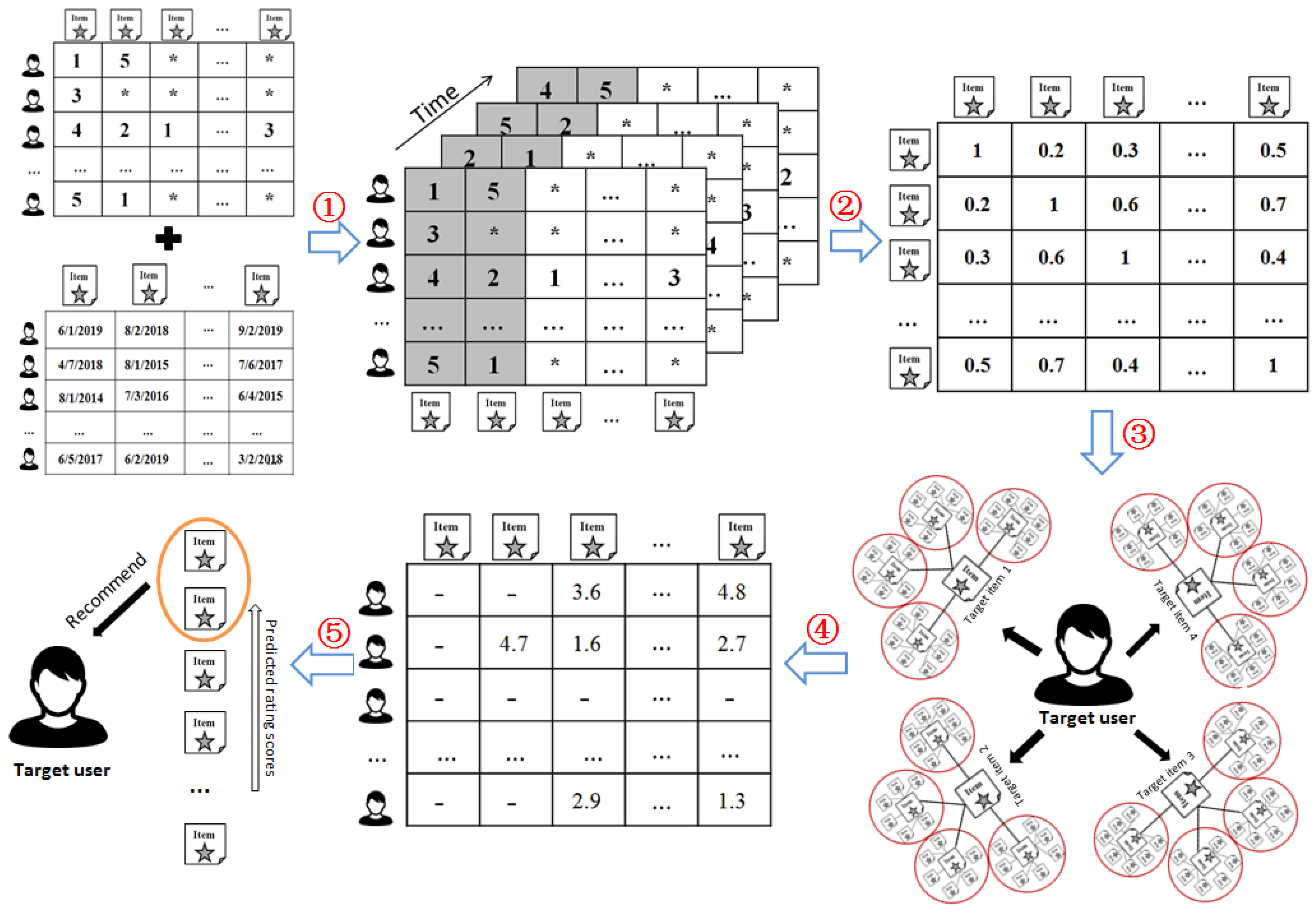
Motivated by this, in this paper, to provide recommendations with good predictive and classification accuracy at the same time, a new approach named TCIBCF was proposed, which implements the time-aware similarity computation and covering-based rating prediction to realize item-variance weighting in traditional IBCF. Figure 1 indicates the flow chart of our proposed approach. We present a time-related correlation degree and apply it to the item-item similarity computation to improve predictive accuracy, that is, recent user ratings are assigned greater weight. We also propose a covering degree and implement it into rating prediction to increase classification accuracy. Items that are closer to a target user’s preference will have a larger covering degree and higher weight. Experimental results demonstrate that the proposed approach outperforms traditional IBCF and other related work and can provide recommendations with satisfactory predictive and classification accuracy. The novel contributions of our approach are featured as follows:

• Different from most related approaches that applied the time factor into rating prediction step [18,19,20], a novel time-related correlation degree function proposed in this paper employs the time factor to compute item-item similarity computation and it can work effectively on the sparse datasets that often occur in real RSs. The predictive accuracy of recommending results can be enhanced effectively by using it and experimental results in Section 4.2 confirm this.
• Unlike the traditional IBCF that utilizes the information of a target item’s similar items to predict rating scores [21,22], the proposed approach further selects neighborhood for each similar item of the target item and presents a new covering degree function to increase the weights of items that are closer to the target user’s preference. By this way, the classification accuracy of recommendations can be improved effectively and experimental results in Section 4.2 confirm this.
• Both predictive and classification accuracy of recommendations are improved. Unlike most related work that can enhance either predictive accuracy or classification accuracy but not in both [18,19,20,21,22], the proposed approach can provide recommendations with satisfactory predictive and classification accuracy simultaneously and experimental results in Section 4 confirm this.

The remainder of this paper is organized as follows. In Section 2, we introduce the traditional IBCF approach and the problem setting. In Section 3, we present the proposed time-aware similarity computation and covering-based rating prediction and provide detailed information about the proposed approach. We describe experiments and compare the results to the traditional IBCF approach and other work in Section 4. Conclusions and suggestions for future work are presented in Section 5.

2. Related Work

2.1. Overview of the Traditional IBCF

First, we explain the notations and terms related to RSs. Given an RS, $U$ and $I$ denote finite sets of users and items, respectively, $R{\cup }^{\text{}}\{\star \}$ denotes the set of possible item rating scores and RM is the user-item rating matrix. $T{\cup }^{\text{}}\{\circ \}$ represents the set of possible item rating time and TM is the user-item time matrix. The rating score of user u for item $x$ is denoted $r_{u,x}\in R{\cup }^{\text{}}\{\star \}$, where $(\star )$ represents a missing rating and $t_{u,x}\in T{\cup }^{\text{}}\{\circ \}$ is the time at which item x was rated by user $u$, where $(\circ )$ indicates a missing rating time. The average of the valid ratings of item $x$ is denoted $r_x$.

The IBCF approach was first proposed by Sarwar [16] and it is widely used in RSs. IBCF has good scalability and can be applied to extremely large numbers of items and users that are typical of modern RSs. In contrast to user-based CF, IBCF can perform well even for RSs that have many items but comparatively few ratings. Furthermore, the IBCF approach can compute item-item similarity offline, which reduces online time and results in more effective recommendations. The IBCF procedure is described in the following.

Step 1: Item-item similarity computation. On the basis of the user-item rating matrix RM, IBCF computes the similarity between all items. Note that several measures can be used to compute similarity; however, we used the Pearson correlation coefficient, which was widely used in IBCF. Similarity computed using the Pearson correlation coefficient is expressed as follows.

$$sim\left(x,y\right)=\frac{{\Sigma }_{u\in U_x{\cap }^{\text{}}{U}_y}\left(r_{u,x}- \overline{r_x}\right)\ast \left(r_{u,y}- \overline{r_y}\right)}{\sqrt{{\Sigma }_{u\in U_x{\cap }^{\text{}}{U}_y}{\left(r_{u,x}- \overline{r_x}\right)}^2} \sqrt{{\Sigma }_{u\in U_x{\cap }^{\text{}}{U}_y}{\left(r_{u,y}- \overline{r_y}\right)}^2}}$$

(1)

Here, $U_x=\left\{u\in U|r_{u,x}\ne \star \right\}$ is a set of users who have rated item x and $\overline{r_y}$ denotes the average rating of item $y$.

Step 2: Neighborhood selection. After computing item-item similarity, for each target item $ti$ that has not been rated by target user $tu$, items with high similarity with target item $ti$ will be selected as its neighborhood. Generally, in traditional IBCF, after all items are sorted in descending order of similarity values, the k most similar (nearest) items will comprise the neighborhood for target item $ti$.

Step 3: Rating prediction. Note that ratings are normalized and according to the rating information of the target item’s neighborhood for target user $tu$, a rating score is predicted for each target item $ti$. Note that the weighted sum is a useful measure often used in the IBCF approach:

$$p_{tu,ti}=\frac{{\Sigma }_{q\in N_{ti}\left(k\right){\cap }^{\text{}}{I}_{tu}}sim\left(t_{i,}q\right)\ast r_{tu,q}}{{\Sigma }_{q\in N_{ti}\left(k\right){\cap }^{\text{}}{I}_{tu}} \left|sim\left(t_{i,}q\right)\right|}$$

(2)

Here, $I_{tu}=\left\{x\in I|r_{tu,x}\ne \star \right\}$ is the set of items rated by target user $tu$, $N_{ti}\left(k\right)$ is the neighborhood of target item $ti$ and $P_{tu,ti}$ is the prediction made about target item $ti$ for target user $tu$.

2.2. Recommendation Accuracy Problem in Traditional IBCF Approach

In the traditional IBCF approach, all items have equal weights for both the item-item similarity computation and rating prediction procedures, that is, item weight is not considered. However, it is widely recognized that some items with greater contribution should be assigned relatively higher weight. Therefore, the traditional IBCF often cannot provide recommendations with good predictive and classification accuracy simultaneously. Figure 2 utilizes two items to describe the comparison between predictive accuracy and classification accuracy. If we treat items rated no less than 3 as relevant items, then, in (a) of Figure 2, both item 1 and item 2 have same classification accuracy; however, because error between prediction and real rating of item 1 is bigger than item 2, item 1 will have worse predictive accuracy than item 2. In (b) of Figure 2, the real rating of item 1 is less than 3 but the predicted rating $p_{u,1}$ is higher than 3, it will result in the classification accuracy of item 1 is worse than item 2. In (c) of Figure 2, both predicted rating and real rating for two items are higher than 3 and errors between them are also the same, so item 1 and item 2 have same results on both predictive accuracy and classification accuracy. From the Figure 2, we can conclude that improving predictive accuracy does not indicate classification accuracy is also improved, vice versa (e.g., (a) and (b) of Figure 2). How to improve predictive and classification accuracy of IBCF simultaneously (e.g., (c) of Figure 2) is a significant problem in the traditional IBCF approach.

To enhance the accuracy of IBCF, a number of approaches have been explored. According to the performance of these approaches, they can be classified into two lines. In the first line, researchers aim to improve the predictive accuracy of IBCF. Gao et al. [21] incorporated the weighted user-rank into the computation of item similarities and differentials to propose a PageRank-based ranking approach, this approach can improve the predictive accuracy of IBCF. Koren [22] proposed a niche approach starting from the dynamic preferences of the target user and extracting the influence on user preferences during the entire time period of user modeling; the predictive accuracy of IBCF has been enhanced clearly by this approach. On the other hand, classification accuracy tries to be improved as a target. Ding et al. [18] applied the time weights for different items in the rating prediction step and increased the weights of the influence of ratings relative to time; this approach could improve the classification accuracy of IBCF effectively. Feng et al. [19] developed a temporal overlapping community detection method based on time-weighted association rule mining; this approach can improve classification accuracy by modeling dynamic user interests. However, even approaches mentioned above can enhance predictive accuracy or classification accuracy of IBCF effectively but they cannot enhance them in both.

3. Proposed Approach

Here, we describe the motivation of the proposed approach. Then, we introduce the time-aware similarity computation and covering-based rating prediction. In addition, we discuss the detailed process and innovative aspects of the proposed approach.

3.1. Motivation

To provide recommendations with better predictive and classification accuracy, the proposed approach attempts to realize item-variance weighting in traditional IBCF, that is, items with greater contribution will have higher weight values in the similarity computation and rating prediction procedures.

In this paper, to increase the predictive accuracy of recommendations, in the similarity computation procedure, we propose a novel time-related correlation function and utilized it to reduce the influence of items rated in the past. Furthermore, to improve the classification accuracy of recommendations, in the rating prediction procedure, for items that have characteristic that are more similar to the target user’s preference, we present a new covering degree to ensure that such items are assigned greater weight.

3.2. Time-Aware Similarity Computation

In an RS, user preferences may change as time goes on, so ratings rated in different period should be assigned different weight [18,19,20]. For example, consider movies 1, 2 and 3 rated by a single person with the same rating scores, where movie 1 was rated one year ago and movies 2 and 3 were rated one day ago. Recall that, in the traditional IBCF, rating weights are equal; thus, here, the similarity between movies 1 and 2 will be the same as that between movies 2 and 3. However, although the ratings have equal values, they may have different contributions because user preferences may change over time. Here, if this user’s preferences have changed, even though movies 1 and 2 are assigned the same rating scores, they may have very different characteristics. Typically, preferences do not change over a single day; thus, movies 2 and 3 should have high similarity. In a similar period, we assume that item ratings can reflect correlation between items more precisely. Therefore, when computing similarity, an effective CF algorithm should gradually reduce the influence of ratings relative to time, that is, recent ratings should be assigned greater weight.

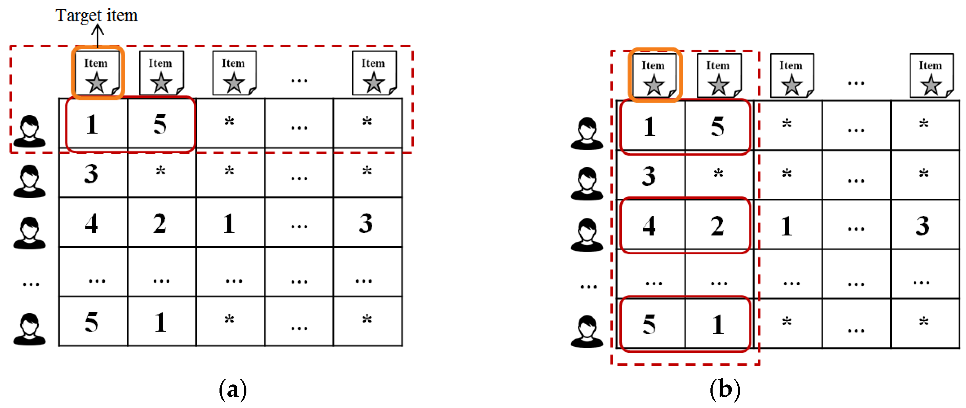
To express the degree of correlation between two items over time, a number of time functions were proposed but most related approaches applied time factor to rating prediction of traditional IBCF (e.g., (a) of Figure 3). However, in this case, the time function was ineffective because, in practical applications, RSs must handle a large amount of data that include significant numbers of users and items. Here, each user has rated only a small number of items compared to the huge number of unrated items. Thus, most RSs have sparse datasets. In the IBCF approach, to maintain real-time performance, the neighborhood size must be limited [23,24,25], that is, the number of items available to rate is limited. The time function is only applied to items that the target user has rated in the target item’s neighborhood; therefore, it is applied to only a few items and cannot efficiently reduce the weight of item ratings given over a long period.

To express the degree of correlation between two items over time more effectively, we propose the following time-related correlation degree in (Equation (3)) that computes time weights for different items such that smaller weight values are assigned to items rated in the past and apply it to the similarity computation in traditional IBCF because, when computing the similarity between each item, it is easy to find two items rated by the same user (e.g., (b) of Figure 3); thus, we can take full advantage of the time-related correlation degree, which is expressed as

$$f\left(u,x,y\right)=e^{-\lambda \ast \left|t_{u,x}-t_{u,y}\right|},$$

(3)

where $\lambda =\frac{1}{T_0}$ is the decay rate. Here, if $T_0=30$ days, the time weight is reduced by one month. $f\left(u,x,y\right)$ is a gradually decreasing function that tracks the degree of correlation between items x and y for target user u. The behavior of the function $f\left(u,x,y\right)$ differs with different values for parameter $T_0$ Thus, we should select different $T_0$ values under different circumstances. For example, consider a dataset with a long-time span (10 years). If we set $T_0$ to one day, most time function values will be 0 and the meaning of the time weight will be lost. In contrast, if a dataset has a short time span (two months) and $T_0$ is set to 30 days, most time function values will be close to 1 and the effect of the time function will be limited.

Generally, user preferences do not change significantly over a short period. Thus, for a single user, the score assigned to an item rated at approximately the same time as the target item will make a greater contribution to effective similarity computation. With the function $f\left(u,x,y\right)$, as the times at which two items were rated by the target user become closer and the value of $\left|t_{u,x}-t_{u,y}\right|$ becomes smaller, the degree of correlation between the two items increases. Therefore, the time-related correlation degree function can effectively estimate the relationship between two items and reduce the weight of the item rated over a long period.

3.3. Covering-Based Rating Prediction

In the traditional IBCF, when predicting the rating score for a target item, items in the neighborhood of the target item will be assigned the same weight values; however, if most of the items in the neighborhood have characteristics that are similar to the target user’s preference, the target item may also be preferred by the target user and should be assigned a relatively higher weight value. The weight differential will result in more accurate prediction results and better recommendations. For example, assume that items $a$ and $b$ are candidates for the target user and that, after sorting items in the neighborhood in descending order of similarity, the similarity values and rating scores for the items in item $a$’s neighborhood will be equal to those of item $b$. However, most items in item $a$’s neighborhood are similar to the target user’s preference and most items in item $b$’s neighborhood have very different characteristics. In traditional IBCF, items $a$ and $b$ will have the same predicted rating scores. However, because the characteristics of item $a$’s neighborhood are more similar to the target user’s preference than those of item $b$, it is more likely that the target user will prefer item $a$. Thus, item $a$ should have a higher predicted rating score than item $b$. In other words, items whose characteristics are more similar to target user’s preference should have higher weight.

In this paper, to measure the relationship between items and the target user’s preference, we present a niche covering degree function (Equation (6)) and further utilize it to propose a covering-based rating prediction method according to the theory of covering-based rough set. As illustrated in Figure 4, different from the traditional IBCF that utilizes the information of a target item’s similar items to predicted rating scores (i.e., (a) of Figure 4), the proposed method further select neighborhood for each similar item of the target item (i.e., (b) of Figure 4) and utilizes proposed covering degree function to increase the weights of items that are closer to the target user’s preference (i.e., (c) of Figure 4).

First, we give the definitions of covering and the covering approximation space. More detailed information can be found in References [26,27,28,29].

Let $T$ be the domain of discourse and $\left\{C_i\right\}\left(i=1,2,\dots ,n\right)$ be a family of subsets of $T$. If $C_i\ne \varnothing$ and ${\cup }^{\text{}}{C}_i=T$, $\left\{C_i\right\}$ is a covering of $T$, denoted by $\mathrm{C}$ and we call the ordered pair $\langle \mathrm{T},\mathrm{C}\rangle$ a covering approximation space.

In a covering approximation space $\langle \mathrm{T},\mathrm{C}\rangle$, the family sets

$$Md\left(t\right)=\left\{K\in C|t\in K\wedge \left(\forall H\in C\wedge t\in H\wedge H\subseteq K\Rightarrow K=H\right)\right\}$$

(4)

is called the minimal description of $t$, which represents a main characteristics description of element $t$. In order to describe the relationship between an element $t\in T$ with a set $X\subseteq T$, Xu and Zhang [26] present a roughness measure in classical rough sets induced by a covering, the definition is as follows.

Let $T$ be the domain of discourse, $C$ be a covering of $T$ and $X\subseteq T$ be a subset of $T$, for every element $t\in T$, degree of rough membership of $t$ in $X$, denote by $D\left(t,X\right)$, is defined by

$$D\left(t,X\right)=\frac{card\left(({\cap }^{\text{}}Md\left(t\right)){\cap }^{\text{}}X\right)}{card\left({\cap }^{\text{}}Md\left(t\right)\right)}$$

(5)

Clearly, for any $t\in T$, $D\left(t,X\right)\in \left[0,1\right]$.

In an RS, an item’s neighborhood is most relevant to the item itself and can express common characteristics of the item. In addition, a target user’s relevant item set can reflect this user’s preference. Here, let $R_{tu}$ be the relevant item set of the target user $tu$, $N_i\left(n\right)$ represents the neighborhood of item $i\in I$ which is comprised by the top $n$ items from the similarity list of item $i$. The covering degree of item $i$ in $R_{tu}$ is defined as

$$CD\left(i,R_{tu}\right)=\frac{card(N_i\left(n\right){\cap }^{\text{}}{R}_{tu})}{card\left(N_i\left(n\right)\right)}$$

(6)

It is clear that $CD\left(i,R_{tu}\right)\in \left[0,1\right]$ and the value of $CD\left(i,R_{tu}\right)$ can be interpreted as the correlation between element $i$ and set $R_{tu}$. Then, we can apply it to the rating prediction procedure and utilize it to measure the relationship between items and the target user’s preference. If an item has a high covering degree, $CD\left(i,R_{tu}\right)$ has a greater value, which means that this item is similar to the target user’s preference; thus, the item should be given greater contribution when predicting the rating score for the target item.

3.4. Procedures of the Proposed Approach

Here, we propose the TCIBCF approach. In the proposed approach, the time-related correlation and covering degree are applied to compute item-item similarity and rating prediction, respectively. Here, $\theta$ is set as the rating score threshold and items with $r_{u,x}\ge \theta$ are defined as relevant items for user $u$. The detailed procedures are described in the following.

Step 1: Time-aware similarity computation. According to user-item rating matrix $\mathrm{RM}$, we insert the time-related correlation degree (Equation (3)) into the Pearson correlation coefficient to compute item-item similarity. Here, we obtain the following:

$$sim\left(x,y\right)=\frac{{\Sigma }_{u\in U_x{\cap }^{\text{}}{U}_y}\left(r_{u,x}- \overline{r_x}\right)\ast \left(r_{u,y}- \overline{r_y}\right)\ast f\left(u,x,y\right)}{\sqrt{{\Sigma }_{u\in U_x{\cap }^{\text{}}{U}_y}{\left(r_{u,x}- \overline{r_x}\right)}^2} \sqrt{{\Sigma }_{u\in U_x{\cap }^{\text{}}{U}_y}{\left(r_{u,y}- \overline{r_y}\right)}^2}}$$

(7)

Step 2: Neighborhood selection. When obtaining the item-item similarity, for each target item $ti$ that has not been rated by target user $tu$, after sorting all items in descending order of similarity, we select the top $k$ items as the neighborhood $N_{ti}\left(k\right)$ of target item $ti$. Furthermore, for each similar item $p\in N_{ti}\left(k\right)$, we select the top $n$ items from the similarity list of item $p$, which comprises the item set $N_p\left(n\right)$.

Step 3: Covering-based rating prediction. In domain $I,$ relevant items for each target user $tu$ comprise the relevant set $R_{tu}$, where

$$R_{tu}=\{x\in I|r_{tu,x}\ge \theta \}$$

(8)

Then, on the basis of the covering degree function (Equation (6)), we compute the covering degree $CD\left(p,R_{tu}\right)$ between each item $p$ and $R_{tu}$ and apply it to the weighted sum approach to predict the rating score of item $ti$ from target user $tu$:

$$p_{tu,ti}=\frac{{\Sigma }_{p\in N_{ti}\left(k\right){\cap }^{\text{}}{I}_{tu}}sim\left(t_{i,}p\right)\ast r_{tu,p}\ast CD\left(p,R_{tu}\right)}{{\Sigma }_{p\in N_{ti}\left(k\right){\cap }^{\text{}}{I}_{tu}} \left|sim\left(t_{i,}p\right)\ast CD\left(p,R_{tu}\right)\right|}$$

(9)

Step 4: Item recommendations. When all predictions for target items are complete, the proposed approach sorts all target items in descending order of predicted rating scores and the top $N$ items are selected as the recommended items for target user $tu$.

3.5. Example of TCIBCF Approach in RSs

Here, we present an example to explain the TCIBCF approach more clearly.

Table 1. Example of user-item rating matrix.

	U1	U2	U3	Utu
I1	3	4	5	1
I2	3	4	5	4
I3	3	4	5	3
I4	3	4	5	2
I5	3	4	5	5
I6	3	4	5	*
I7	3	4	5	*

shows a user-item rating matrix by four users for seven items. The user set is comprised by $\left\{U_1,U_2,U_3,U_{tu}\right\}$, where $U_{tu}$ means the target user. The item set consists of $\left\{I_1,I_2,I_3,I_4,I_5,I_6,I_7\right\}$. The rating value is from 1 to 5, where a higher value indicates that the user likes the given item more.

Table 2. Example of user-item time matrix.

	U1	U2	U3	Utu
I1	6/1/2018	6/1/2018	6/1/2018	6/1/2018
I2	5/1/2018	5/1/2018	5/1/2018	5/1/2018
I3	4/1/2018	4/1/2018	4/1/2018	4/1/2018
I4	3/1/2018	3/1/2018	3/1/2018	3/1/2018
I5	2/1/2018	2/1/2018	2/1/2018	2/1/2018
I6	2/1/2018	2/1/2018	2/1/2018	◦
I7	6/1/2018	6/1/2018	6/1/2018	◦

illustrates a user-item time matrix which shows the time that the user gave the rating in Table 1 and we take one day as a unit of rating time.

In the traditional IBCF approach, because $I_6$ and $I_7$ have the same rating scores from $\left\{U_1,U_2,U_3\right\}$, respectively, thus they will have the same neighborhood and predicted rating scores. However, $I_6$ and $I_7$ may have different rating time and characteristics, so they should have different recommended order for the target user $tu$. In our proposed TCIBCF approach, after the time-aware similarity and covering-based rating prediction, neighborhood and predicted rating scores are quite different between $I_6$ and $I_7$. The detailed procedures of TCIBCF are as follows.

Step 1: Time-aware similarity computation. In order to compute the time-related correlation degree (Equation (3)), we treat $T_0=30$ days in $\lambda =\frac{1}{T_0}$, it means the time weight is reduced by one month. Then, we use Equation 7 to compute item-item similarity,

Table 3. Example of item-item similarity with time-related correlation degree.

	I1	I2	I3	I4	I5	I6	I7
I1	1	0.176	0.091	0.049	−0.001	0.013	0.736
I2	0.176	1	0.314	0.086	0.016	0.050	0.368
I3	0.091	0.314	1	0.288	0.062	0.129	0.129
I4	0.049	0.086	0.288	1	0.050	0.314	0.042
I5	−0.001	0.016	0.062	0.050	1	0.956	0.017
I6	0.013	0.050	0.129	0.314	0.956	1	0.368
I7	0.736	0.368	0.129	0.042	0.017	0.368	1

shows the result of item-item similarity with time-related correlation degree.

Step 2: Neighborhood selection. After obtaining the item-item similarity, we set the size of item’s neighborhood as 3, then, the neighborhood of each item is as follows:

$$N_1\left(3\right)=\left\{I_7,I_2,I_3\right\}; N_2\left(3\right)=\left\{I_7,I_3,I_1\right\};$$

$$N_3\left(3\right)=\left\{I_2,I_4,I_6\right\}; N_4\left(3\right)=\left\{I_6,I_3,I_2\right\};$$

$$N_5\left(3\right)=\left\{I_6,I_3,I_4\right\}; N_6\left(3\right)=\left\{I_5,I_7,I_4\right\};$$

$$N_7\left(3\right)=\left\{I_1,I_2,I_6\right\}$$

Step 3: Covering-based rating prediction. Here, we treat item whose rating is great than or equal to 3 as the target user’s preferred item, then, the target user’s preferred item set is $R_{tu}=\left\{I_2,I_3,I_5\right\}$. According to the covering degree we proposed, we compute the covering degree between each item and the target user’s preferred item set $R_{tu}$:

$$CD\left(I_1,R_{tu}\right)=2/3; CD\left(I_2,R_{tu}\right)=1/3;$$

$$CD\left(I_3,R_{tu}\right)=1/3; CD\left(I_4,R_{tu}\right)=2/3;$$

$$CD\left(I_5,R_{tu}\right)=1/3; CD\left(I_6,R_{tu}\right)=1/3;$$

$$CD\left(I_7,R_{tu}\right)=1/3.$$

Then, we utilize Equation 9 to predict the rating score for $I_6$ and $I_7.$ Here $P_{U_{tu},I_6}$ = 3.811, $P_{U_{tu},I_7}$ = 1.600.

Step 4: Item recommendations. Because $P_{U_{tu},I_6}>P_{U_{tu},I_7}$, if we select the top one movie as recommendation, $I_6$ will be recommended to the target user $tu$.

3.6. Discussion

The most significant innovation in the proposed approach is its ability to realize item-variance weighting in traditional IBCF. Here, as a key item can play a more significant role in RSs, the recommendations provided to the target user could have satisfactory predictive and classification accuracy.

The proposed approach employs two techniques to utilize item-variance weighting to improve predictive and classification accuracy in traditional IBCF.

• The time-related correlation degree is applied to the similarity computation procedure to improve predictive accuracy.
• The covering degree is applied to the rating prediction procedure to improve classification accuracy.

Relative to the first technique, we note that a user’s interests may change over time. In traditional IBCF, items rated at different times have the same weight. Thus, some items rated by the user in the past will have the same weight as recently rated items, even if the target user has changed his or her preferences. The time-related correlation degree function can most effectively reduce the weight of items rated by a user over a long period. Thus, we can reduce the effects of changing user preferences over time. After applying the time-related correlation degree to the similarity computation, items recently rated by the same user will have greater weight than items rated in the past. Thus, the similarity can reflect the relationship between items more precisely. Therefore, errors between the predicted and real ratings are reduced and predictive accuracy is improved.

Relative to the second technique, in traditional IBCF, items in the neighborhood of the target item will have the same weight. In other words, when predicting the rating score for a target item based on rating information from the item’s neighborhood, items that are more similar to the target user’s preference will have the same weight as items that differ significantly from the target user’s preference. Therefore, some items preferred by the target user cannot have higher predicted rating scores than others and it will be difficult to be recommend such items to the target user. The covering degree can measure the relationship between items and the target user’s preference. Thus, after applying the covering degree to rating prediction, items that are more similar to the target user’s preference will have greater weight than others, which means that these items will have greater contribution when predicting rating scores. As a result, target items with more neighborhoods that are similar to the target user’s preference and may be preferred by the user will have relatively higher predicted rating scores. Consequently, it becomes easy to recommend such items to the target user. Therefore, the proposed approach can improve the classification accuracy of recommendations.

Note that, different from some related approaches which require additional information (e.g., user profiles) that is often not available or incomplete [18,19,20,21,22,23], our proposed TCIBCF approach can output recommended items for target user $tu$ without needing other special information.

4. Experiments and Evaluation

In this section, we introduce the evaluation datasets and metrics, examine the effects of the proposed approach and compare the performance of the proposed approach to that of other work.

4.1. Experimental Setup and Evaluation Metrics

Here, we used two popular real-world datasets that are often used to evaluate RSs. One is the MovieLens10M dataset [30], which was collected by the GroupLens Research Project from January 1995 to January 2009 (168 months). This dataset contains 10,681 movies, 69,878 users and a total of 10 million ratings on a scale of $\left\{0.5,1,1.5,2,2.5,3,3.5,4,4.5,5\right\}$. In this dataset, each user has rated at least 20 movies. The other dataset is the Netflix dataset obtained from the Netflix Prize website (http://www.netflixprize.com). This dataset was collected between October 1998 and December 2005 (85 months) and it contains a total of 100 million ratings of 17,770 movies from 480,189 users. The ratings are on a $\left\{1,2,3,4,5\right\}$ scale and each user has rated a different number of movies.

In this paper, considering the huge number of items and users in the MovieLens10M and Netflix dataset, to obtain a manageable size, for each dataset, we randomly selected 2000 items as the experimental data. In our experiment, in order to mimic real-world conditions, we utilized one of the most popular rating orders: the user-centered and time-dependent ordering conditions combination to build the training and test sets [20]. For each item, we ordered the ratings by timestamps separately and the most recent 20% of the ratings were treated as test data and the remaining 80% were treated as training data. We used the training data to compute the item-item similarity and predicted rating scores for the test data and the test data were used to evaluate the performance of the proposed approach. As the MovieLens10M dataset was collected over 168 months, we used two months period (60 days) as the time decay rate. As the Netflix data were collected over 85 months, we utilized a month period (30 days) as the time decay rate. To avoid the impact of accidental phenomena, we repeated experiments for each dataset 20 times and computed the average values as the results.

In RSs, the customer’s confidence in the system depends on both the predictive accuracy and classification accuracy. Therefore, in our experiments, we used the mean absolute error (MAE) and root-mean-square error (RMSE) to represent the predictive accuracy of recommendations. In addition, we used precision, recall and F1 measures to represent the classification accuracy of recommendations.

The MAE and RMSE metrics demonstrate the average error between predictions and real values; therefore, lower values represent higher accuracy. The MAE and RMSE are expressed as follows:

$$MAE= \frac{1}{card\left(U\right)}\sum _{u\in U}(\frac{1}{card\left(O_u\right)}\sum _{x\in O_u}\left|p_{u,x}- r_{u,x}\right|)$$

(10)

$$RMSE= \frac{1}{card\left(U\right)}\sum _{u\in U}\sqrt{\frac{1}{card\left(O_u\right)}\sum _{x\in O_u}{\left(p_{u,x}- r_{u,x}\right)}^2}$$

(11)

where $O_u=\{x\in I|p_{u,x}\ne \star \wedge r_{u,x}\ne \star \}$ indicates a set of items rated by user $\mathrm{u}$ with prediction values.

Precision refers to the proportion of relevant recommended items from the total number of recommended items for the target user. Here, higher values indicate better performance. Assuming that $N_s$ is the number of recommended items for the target user, $N_{rs}$ denotes the amounts of items the target user likes that appear in the recommended list. The precision metric is defined as follows:

$$Precision=\frac{N_{rs}}{N_s}$$

(12)

Recall indicates the proportion of relevant recommended items from all relevant items for the target user. Similar to precision, higher recall values indicate better performance. Here, $N_r$ denotes the number of items preferred by the target user. The recall metric is computed as follows:

$$Recall=\frac{N_{rs}}{N_r}.$$

(13)

F1 is a combination of precision and recall expressed as follows:

$$F1=\frac{2\ast Precision\ast Recall}{Precision+Recall}$$

(14)

Note that neighborhood size has a significant impact on recommendation quality [23,24,25]. According to previous research [16], 30 is an optimal neighborhood size; thus, in our experiments, we set $\mathrm{n}=30$ for each item in the target item’s neighborhood, which means that we utilized an item’s top 30 most similar items to represent the given item’s characteristics. However, to indicate changes in the evaluation metrics as the size of the target item’s neighborhood increases, we also used different neighborhood sizes $\left\{10,20,30,40,50\right\}$. Furthermore, to calculate the precision, recall and F1 values, we treated items rated no less than 3 as relevant items and the number of recommendations was set to 2, 4, 6, 8, 10 and 12.

4.2. Experimental Results and Comparisons

We further define TCIBCF to represent the proposed approach using the time-aware similarity computation and covering-based rating prediction, TRIBCF to represent IBCF only using the time-aware similarity computation and CDIBCF to represent IBCF only using the covering-based rating prediction. To demonstrate the performance of the proposed TCIBCF approach and the effect of TCIBCF’s different components, we compared our results to TRIBCF approach and CDIBCF approach. In addition, we also compared the proposed approach to the traditional IBCF approach and time-weight item-based collaborative filtering (TWIBCF) proposed by Ding [13]. In all experiments, we used the Pearson correlation coefficient as the similarity measure and the weighted sum was used to predict the rating score.

Figure 5 and Figure 6 show the MAE and RMSE results for the MovieLens and Netflix datasets. As can be seen, with increasing neighborhood size, both MAE and RMSE initially decrease then increase with both datasets. With the MovieLens dataset, the MAE and RMSE values between IBCF and CDIBCF are almost the same and the same performance happens in TCIBCF and TRIBCF approaches; however, the MAE and RMSE values of the TCIBCF approach are less than IBCF and TWIBCF approaches. As lower values indicate better predictive accuracy, these results show that time-related correlation can enhance the predictive accuracy, covering degrees have no effect on enhancing the predictive accuracy, so TCIBCF has improved predictive accuracy compared to the traditional IBCF and TWIBCF approaches. With the Netflix dataset, although the values of the evaluation metrics differed, the performance of those approaches was nearly the same as that with the MovieLens dataset. From the above results, we conclude that the time-related correlation can improve predictive accuracy effectively and the predictive accuracy of the proposed TCIBCF approach is better than that of the traditional IBCF and TWIBCF approaches.

Figure 7 shows the precision results obtained with the MovieLens and Netflix datasets, respectively. As can be seen, the precision values for those approaches decreased as the neighborhood size increased. Furthermore, the precision values of the IBCF, TRIBCF and TWIBCF approaches were nearly the same and the same performance for TCIBCF and CDIBCF; however, the precision of the TCIBCF and CDIBCF approaches were clearly greater than that of IBCF, TRIBCF and TWIBCF approaches.

Figure 8 shows the recall results obtained with the MovieLens and Netflix datasets, respectively. As can be seen, recall increased as the neighborhood size increased with both datasets. TWIBCF and TRIBCF approaches demonstrated nearly the same performance as traditional IBCF, indicating that TWIBCF and TRIBCF cannot improve recall compared to traditional IBCF. However, the recall of TCIBCF and CDIBCF increased faster than the traditional IBCF approach. Moreover, the improvement became larger as the neighborhood size increased. Thus, TCIBCF and CDIBCF can improve the recall of traditional IBCF and outperforms TWIBCF and TRIBCF approaches. Figure 9 shows the F1 results for the MovieLens and Netflix datasets, respectively. As shown, the F1 value increased as the neighborhood size increased with both the MovieLens and Netflix datasets. With the MovieLens dataset, first, all of those approaches showed nearly the same F1 values; however, as the neighborhood size increased, the F1 value of TCIBCF and CDIBCF increased faster than that of the traditional IBCF, TRIBCF and TWIBCF approaches. With the Netflix dataset, the F1 values of TCIBCF and CDIBCF were almost the same; however, the F1 values of TCIBCF and CDIBCF were always greater than that of the other three approaches. Thus, the proposed TCIBCF improved F1 results compared to the traditional IBCF and other related work.

The precision, recall and F1 results obtained with the MovieLens and Netflix datasets indicate that, through the use of covering degrees, classification accuracy can be enhanced effectively, so the proposed TCIBCF can improve the classification accuracy of the traditional IBCF and other related work, which means that the recommendations provided by the proposed TCIBCF approach will be more relevant to the users.

4.3. Discussion

In the proposed approach, items are assigned different weights in the item-item similarity computation. For example, consider two items x and y with the same rating scores from user $u$ (i.e., $r_{u,x}=r_{u,y}$). Here, the time at which the user u rated target item $ti$ is $t_{u,ti}$. In addition, item x is more recent than the rating time of item y, that is, $\left|t_{u,ti}-t_{u,x}\right|<\left|t_{u,ti}-t_{u,y}\right|$. In a traditional IBCF, items $x$ and $y$ will be given the same similarity as target item $ti$, because they received the same rating score from the user $u$. However, the preferences of user $u$ may have changed over time; thus, the rating of item $x$ will have greater influence than that of item $y$. In the proposed approach, $f\left(u,ti,x\right)>f\left(u,ti,y\right)$; thus, item $\mathrm{x}$ will obtain higher similarity with the target item than item $\mathrm{y}$ after computing the item-item similarity. In this manner, items that have greater influence on the target item will be selected for the target item’s neighborhood. Here, the items selected as the neighborhood of the target item are more reliable; thus, the neighborhood selected by TCIBCF is more similar to the target item than that of traditional IBCF and this reduces error between the predicted and real ratings. Therefore, the proposed TCIBCF approach provided recommendations with better predictive accuracy than traditional IBCF and other related work for both the MovieLens and Netflix datasets.

After computing the similarity, items that are similar to the target item were selected to predict the rating score. Here, we used the covering degree function to compute the weight of each similar item. For each item $p$ in the target item’s neighborhood, item set $N_p\left(n\right)$ captured its characteristics. If $N_p\left(n\right)$ has a greater degree of inclusion in the target user’s preferences $R_{tu}$, such that the value of $CD\left(N_p\left(n\right),R_{tu}\right)$ is high, this suggests that the characteristics of item $p$ are nearer to the target user’s preferences. If the target item’s neighborhood includes many such items, this target item is more likely to be preferred by the target user. For this target item to obtain a higher predicted rating score, item $p$ will therefore be assigned greater weight than other items when performing rating prediction. Thus, if a target item’s neighborhood includes more items with a high covering degree, the target item is more likely to be preferred by the target user and as this item will have a higher predicted rating score, it becomes easy to recommend this item to the target user. Therefore, most of items in the target user’s recommendation list will be preferred items and the classification accuracy of the proposed approach will be better than that of traditional IBCF and other related work. In summary, recommendations obtained by the proposed approach show accurate predicted rating scores and are preferred by the target user; thus, the proposed approach is more suitable for real-world RS application.

5. Conclusions and Future Work

In this paper, we have proposed the TCIBCF approach to realize item-variance weighting in traditional IBCF. The proposed TCIBCF applies time-related correlation and covering degrees to traditional IBCF to ensure that item weights make a significant contribution to the similarity computation and rating prediction processes. We have shown that the proposed approach outperforms the traditional IBCF approach and other related work experimentally, relative to both predictive accuracy and classification accuracy. To ensure that items with greater impact will have higher weight, the proposed approach realizes the item-variance weighting for traditional IBCF and achieves significant improvements in predictive and classification accuracy while utilizing only the user-item rating matrix rather than any other special information.

The proposed approach can be applied to the new item cold-start issue, which is a very difficult problem in RSs, where a new item has only been rated by a few users; thus, sufficient information cannot be obtained from the new item, which increases the difficulty of making recommendations. Applying the proposed approach to the new item cold-start issue will be our next work. Besides that, more detailed analysis of the proposed approach with data scalability and comparison with more complex recommendation approaches (e.g., graph analysis, deep learning, etc.) will be our future work.