Soft Sensor with Adaptive Algorithm for Filter Gain Correction in the Online Monitoring System of a Polluted River

Abstract

This paper proposes the realization of a soft sensor using an adaptive algorithm with proportional correction of the gain coefficient for monitoring river water quality. This algorithm makes it possible to monitor online signals of an object described by nonlinear ordinary differential equations. Simulation studies of a biochemically polluted river, for which the water quality was represented by biochemical oxygen demand (BOD) indices and the dissolved oxygen (DO) deficit, were carried out. The algorithm concept uses only online measurements of the object, and adaptive changes in the gain coefficient are determined based on the adaptation error adopted for this purpose. Simulation results indicated the correct functioning of the soft sensor even for inaccurately identified parameters of the mathematical model and for unknown values and intensity of disturbances affecting the object. The quality of the signals monitored via a soft sensor implemented in this way was determined with the root-mean-squared error (RMSE) and mean percentage error (MPE) indicators and compared with the Kalman filter.

1. Introduction

The problem of monitoring objects via a real-time system is still a topical and important issue for the industry connected with ecological systems. The need to control the quality of surface water is primarily due to the necessity of protecting the natural environment. The increasing level of water pollutants is mainly associated with the rapid increase of social development. As a result of these transformations, the need for functioning wastewater treatment plants with much higher requirements in terms of quality and efficiency of operation has arisen. In addition to the impact of the treatment plant, weather conditions also have a big influence on the quality of water in rivers, which in turn leads to the need for continuous monitoring with a control and management function to ensure the possibility of managing water in a given region [1,2].

Real-time monitoring systems, which are additionally used for monitoring and control functions, also require fast and accurate determination of the desired signal values. This is achieved by applying various methods and techniques related to the necessity of carrying out the key computer calculations. The simplest monitoring solutions only use easily implementable online measurements, which are part of a full monitoring system, as no other signals of the object are taken into consideration [3]. The proposition for the estimation of water quality presented in [4] uses artificial neural networks and canonical correlation analysis to ensure the correctness of water quality assessment. These considerations include numerous water quality parameters but determine only their static parameters. With this approach, we were not able to observe the dynamic changes in water quality resulting from random extortions. A similar approach was presented in [5], in which the authors developed and proposed methods for assessing water quality for management purposes of local governments, with data obtained on a weekly or annual basis. However, this solution did not take into account the impact of anomalous pollution changes, which indicates the need for continuous online measurements.

In [6], the authors proposed real-time monitoring based on online measurements using mobile measurement stations. This type of mobility does not ensure continuous comprehensive monitoring of water quality in a given water catchment. Other solutions concern the monitoring and control system involving interaction with the object. Such hybrid solutions lead to positive results but at the cost of larger computational effort associated with the current “improvements” of the characteristics of stochastic signals [7,8,9,10].

In monitoring systems, soft sensors are often used to obtain information about certain parameters, which are produced on the basis of measurements of other signals. The principle of soft sensing technology is to build a mathematical model to estimate signals which are difficult to measure, based on the relationship between these signals and certain online signals measured directly. An approach implementing such a soft sensor was presented, among others, in [11,12,13].

The first study previously mentioned used genetic algorithms to control the value of dissolved oxygen (DO) in a wastewater treatment plant. The authors obtained the right quality of sewage and minimized the energy demand, which is a valuable achievement for an integrated global monitoring system with the control function. The second and third mentioned works considered a control system for which the controller’s parameters were selected using an artificial neural network or extreme learning machine (ELM). Satisfactory results were obtained in the form of good real-time performance and high accuracy of soft sensor prediction.

Solutions which are not based on artificial neural networks can also give positive results, even for nonlinear objects [14]. There has been research done on a soft sensor based on locally weighted regression which estimates the regression surface by multivariate smoothing. The implementation of a soft sensor generating a biochemical oxygen demand (BOD) signal for water in an open system based on measurements of many signals and the use of a self-organizing neural network with random weights was presented in [15]. An additional requirement of this application is the preprocessing of data.

Soft sensors can also be implemented using Kalman filter algorithms [16]. This approach used measurements from two different sources to obtain the estimated signal sought, and in the Kalman algorithm, the stages of prediction and updating of the signal estimation were separated. The final results of the soft sensor were based on measurements of online signals and signals developed in laboratory tests, which imposed an additional load on the proposed method.

An extended Kalman filter was used in [17] to obtain better results. The methods used there, in the form of Monte Carlo or polynomial chaos theory, give hope for improvement of the computational efficiency of methods for estimating current parameters but at the cost of greater computational complexity.

The studies discussed above present different approaches for achieving appropriate improvements in the quality of final results, however, they are burdened with significant computational inputs.

This article proposes an adaptive approach to the implementation of the soft sensor, enabling generation of desired signals describing the object, obtained on the basis of possible online measurements and signals generated from a mathematical model. This approach is characterized by lower computational complexity and greater accuracy of the solution compared with algorithms using Kalman filters mechanisms. The essence of the proposed adaptation mechanism consists of changing the gain coefficient in time in the soft sensor’s filtration equation used for online monitoring of river water quality.

2. Concept of a Monitoring System Using a Mathematical Model

BOD and DO are considered to be important indicators of water pollution [1,2,18]. The values of these indicators in river waters change despite properly functioning wastewater treatment plants. This is a result of laterally distracted and point tributaries and weather conditions such as rainfall. For the purposes of monitoring, control, or simulation tests, a mathematical model is usually used, which represents the description of these impurities in the form of ordinary or partial differential equations representing the kinetics of first-order physicochemical reactions [19].

The BOD indicator can be described by an equation in the following form:

$$\frac{d}{dt}{x}_1\left(t\right)=-k_1{x}_1\left(t\right)+w_1$$

(1)

while the DO deficit indicator can be expressed by dependence:

$$\frac{d}{dt}{x}_2\left(t\right)=-k_2{x}_1\left(t\right)-k_3{x}_2\left(t\right)+w_2$$

(2)

where $x_1,x_2$ are, respectively, indicators of water quality BOD and DO;

• $k_1$—coefficient rate of BOD reaction;
• $k_2$—coefficient influence of BOD to DO;
• $k_3$—coefficient of change of oxygen deficit in water;
• $w_1$—intensity of inflow of BOD pollutants;
• $w_2$—intensity of oxygen uptake/delivery from/to water.

Equations (1) and (2) transformed into a vector form can be expressed by the following equation:

$$\frac{d}{dt}x\left(t\right)=\mathit{A}x\left(t\right)+\mathit{B}w\left(t\right)$$

(3)

where:

• $x=\left[\begin{array}{c}{x}_1\\ x_2\end{array}\right]$—vector representing water quality indicators;
• $\mathit{A}=\left[\begin{array}{c}{k}_1\\ k_2\end{array}\begin{array}{c}0\\ k_3\end{array}\right]$—dynamics matrix of vector changes $x$;
• $w=\left[\begin{array}{c}{w}_1\\ w_2\end{array}\right]$—disturbance vector of system;
• $\mathit{B}=\left[\begin{array}{cc}1& 0\\ 0& 1\end{array}\right]$—interactions matrix of disturbance signals.

The existing BOD pollution in a river causes an increase in the DO deficit due to biochemical processes which use the oxygen contained in the water. After a certain period, the pollution in the form of BOD and deficit of oxygen in the form of DO decrease as a consequence of the river’s natural self-purification process. Coefficients contained in matrix A describe the dynamics of a river’s self-purification process and depend on temperature (the seasons of the year) and, therefore, they are not constant values but are subject to change in certain ranges [20]:

$$\begin{gathered} k_1=-0.2204÷-0.3347[\mathrm{mg}/\mathrm{L}], \\ {k}_2=-0.1636÷-0.2049[\mathrm{mg}/\mathrm{L}], \\ {k}_3=-0.71÷-0.81[\mathrm{mg}/\mathrm{L}]. \end{gathered}$$

(4)

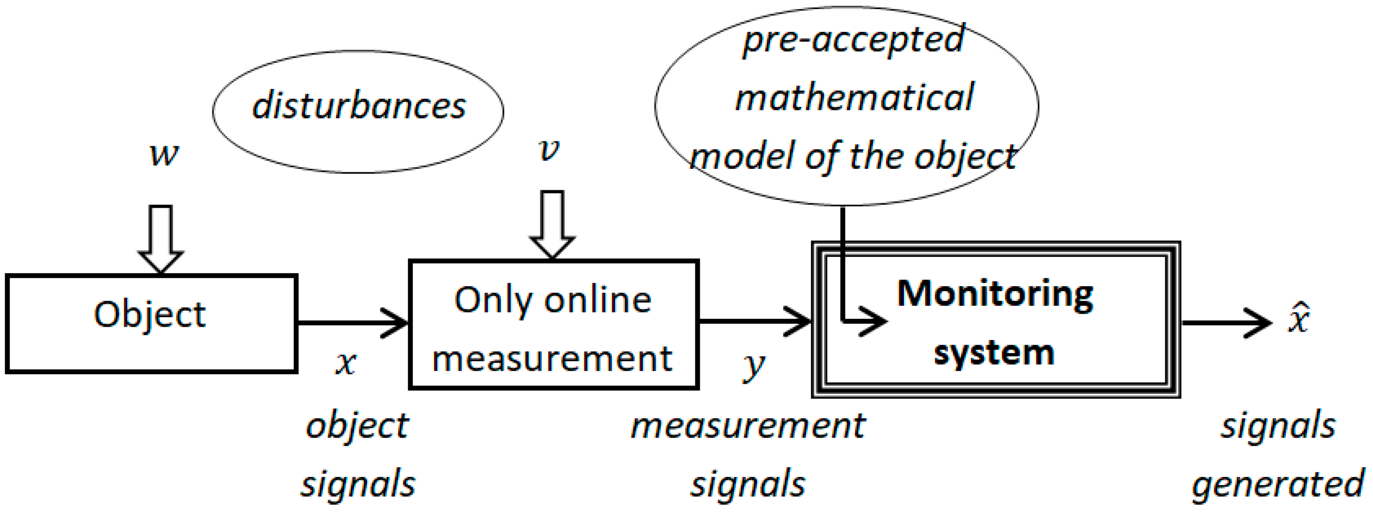
Accepting such assumptions causes the mathematical model defined by Equation (3) to ultimately become a nonlinear model, although in certain temperature ranges, it can be assumed as linear. Equation (3) of the presented model was applied in the soft sensor for the monitoring system that generated real object signals. The idea of this approach is presented in Figure 1.

The monitoring system based on a soft sensor uses a preaccepted mathematical model of the object and the proposed adaptive algorithm which generates signals based on object signals measurable online.

As mentioned above, there are two signals which can be considered as part of the water quality issue (i.e., BOD and DO deficits). Measurements of the DO deficit can be obtained online with the help of an oxygen probe, whereas BOD measurements require laboratory service. In practice, the time required to obtain such results is 5–20 days. In the case of online monitoring, such measurement becomes useless and, therefore, it has been withdrawn from in favor of constructing an algorithm that recreates its values. This approach was used in the presented studies.

Therefore, it is only necessary to measure the DO deficit, which is described by the equation in the following form:

$$y\left(t\right)=\mathit{C}x\left(t\right)+\mathit{v}\left(t\right)$$

(5)

where:

• $\mathit{C}=\left[01\right]$—measurement matrix;
• $\mathit{v}$—measurement error matrix.

Configuration of measurement matrix C indicates the selection of measurement DO, which will be the only information regarding the quality of water. On the other hand, the task of the monitoring algorithm will be to generate a substitute signal representing the BOD value using an adaptive approach in soft sensor implementation.

3. Concept of an Adaptive Algorithm of Proportional Gain Change

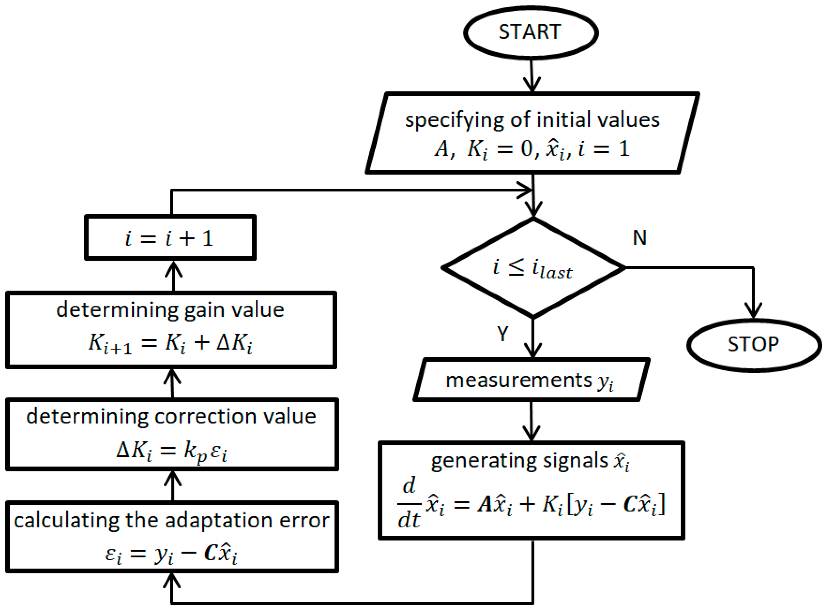
The proposed adaptive P-type gain change algorithm for the soft sensor generates all object signals, including those for which no measurements can be made due to the difficulties of online measurement. The concept of the algorithm consists of applying a filtration equation with a structure used that is similar to the Kalman filter. However, the value of the gain will be determined adaptively. In particular, modification of the gain coefficient is made in each step of the calculation based on the current adaptation error ${\epsilon }_i$ (7), defined for the needs of this algorithm.

The equation generating the signals of the object in the monitoring system takes the form

$$\frac{d}{dt}{\widehat{x}}_i=\mathit{A}{\widehat{x}}_i+K_i\left[y_i-\mathit{C}{\widehat{x}}_i\right]$$

(6)

where:

• $\widehat{x}$—signal generated by soft sensor adaptive algorithm;
• $y$—measurements from Equation (5);
• $\mathit{A}$—matrix from the model (3);
• $K$—adaptively determined values of the gain coefficient;
• $\mathit{C}$—measurement matrix;
• i—index of the current calculation step.

The adaptation error is a real, measurable signal, expressed by the equation

$${\epsilon }_i=y_i-\mathit{C}{\widehat{x}}_i$$

(7)

where ${\epsilon }_i$ is the adaptation error in the ith step.

Based on the adaptation error defined in this way, the algorithm determines the proportional correction value of the gain coefficient dependent on the adaptation error value according to the equation

$$\Delta K_i=k_p{\epsilon }_i,$$

(8)

in which:

• $\Delta K$—correction of the gain coefficient;
• $k_p$—proportionality parameter of changes in the gain coefficient.

At the present stage of research, expert knowledge is required to determine the value of parameter $k_p$ contained in Equation (8).

After determining the correction, the current value of the $K$ gain coefficient is determined incrementally in each calculation step according to the dependence:

$$K_{i+1}=K_i+\Delta K_i,K_0=0.$$

(9)

Assumption of the initial value of the gain coefficient is zero. This causes greater universality of applications of the proposed adaptive algorithm.

The gain thus obtained is used in Equation (6) to generate all the approximated signals of the object, even signals for which no measurements are made. In Equation (8), the error value ${\epsilon }_i$ represents the current information about the discrepancy between the signals of the $x_i$ object and the value generated in the soft sensor ${\widehat{x}}_i$(see Figure 1). Thus, the current value of the gain correction $\Delta K_i$ results from the value of the adaptive error, which indicates the need to change the gain $K_i$ to reduce the error ${\epsilon }_i$. The general concept of the algorithm used in the soft sensor is shown in the block diagram in Figure 2.

The algorithm generates ${\widehat{x}}_i$ signals representing all signals of the object based on measurements $y_i$ made only in online mode. The left part of the algorithm diagram determines the current values of gain coefficient $K_i$ affecting the quality of the generated signals.

The proposed algorithm requires knowledge of the mathematical model, but parameters of the object do not need to be determined precisely. An important advantage of the presented algorithm is the stability of operation for any values of interference generated on the basis of their intensity (lack of information about statistics characteristics for these signals). The soft sensor based on the proposed algorithm works in online mode and can generate signals with satisfactory accuracy, even for such signals for which no measurements are made.

Computational Complexity of the Adaptive Algorithm

Computational complexity of the soft sensor was determined in accordance with the diagram shown in Figure 2.

Table 1. Computational complexity of the adaptive algorithm.

	Calculation	Specificity of Calculations	Complexity
1	Equation solution	$\frac{d}{dt}\widehat{x}=\mathit{A}\widehat{x}+K_A\left[y-\mathit{C}\widehat{x}\right]$	$2n^2+4n$
2	Adaptation error	$\epsilon =y-\mathit{C}\widehat{x}$	$n^2+2n$
3	Gain correction	$\Delta K=k_p\epsilon$	$2n$
4	Gain value	$K_A=K_S+\Delta K$	$2n$
		Total:	$3n^2+10n\in \mathit{O}\left({\mathit{n}}^2\right)$

and

Table 2. Computational complexity of the Kalman filter algorithm.

	Calculation	Specificity of Calculations	Complexity
1	The Riccati equation 1 solution	$\frac{d}{dt}\mathit{P}=\mathit{A}\mathit{P}+\mathit{P}{\mathit{A}}^T-\mathit{P}{\mathit{C}}^T{\mathit{V}}^{-1}\mathit{C}\mathit{P}+\mathit{D}\mathit{W}{\mathit{D}}^T$	$8n^3+3n^2+4n$
2	Gain value	$K_F=\mathit{P}{\mathit{C}}^T{\mathit{V}}^{-1}$	$3n^3+n^2+n$
3	Equation solution	$\widehat{x}=\mathit{A}\widehat{x}+K_F\left[y-\mathit{C}\widehat{x}\right]$	$2n^2+4n$
		Total:	$11n^3+6n^2+9n\in \mathit{O}\left({\mathit{n}}^3\right)$

¹P—estimation error covariance matrix, V—measurement error covariance matrix, W—system disturbances covariance matrix, D—disturbances interaction matrix.

provide details on signal calculation and the complexity of these calculations. Detailed computational complexity of the algorithms results from the following parameters and operations: dimension of system vector—n; matrix multiplication—O($n^3$); matrix transpose—O($n^2$); matrix inversion—O($n^3$); additions, subtractions, and assignments—O(n); and multiplication of matrix and vector—O($n^2$).

The largest complexity in the adaptive algorithm comes from the multiplication of the matrix and the vector, and this is the complexity of order O($n^2$).

For special algorithms, the computational complexity of matrix multiplication is $\mathit{O}\left({\mathit{n}}^{2.373}\right)$ [21].

In the Kalman filter algorithm, the greatest complexity results from the multiplication and inversion of the matrix, which in effect gives the complexity of the order O($n^3$). The adaptive approach used only simple calculations; hence, a lower order of computational complexity was obtained compared with the Kalman filter algorithm.

The algorithm presented in this article is characterized by lower computational complexity in relation to the classical approach (i.e., the Kalman filter) because there is no need to determine the gain coefficient by solving the Riccati nonlinear differential equation [7,9,16,22,23].

The approach to generating signals realized with artificial neural networks has been shown in [10]. In this case, there is comparable computational complexity, but it does not guarantee obtaining the correct signal quality. It results from the necessity of carrying out the learning process for cases representing the most characteristic extortion, which is a difficult issue. In addition, the computational complexity of the network learning process is greater than the normal network operation, although it is done offline.

4. Simulation Research Results

The presented simulation studies concern the time courses of BOD and DO signals obtained from the mathematical model and signals generated by the proposed adaptive algorithm, as well as the Kalman filter. The results also apply to cases in which the parameters of the real object and the mathematical model which was used to generate signals were different. The results of the tests also include time courses of errors of the abovementioned algorithms. The final part of the research presents averaged indicators of monitoring quality (10, 11) and the results of comparing the computational complexity of the adaptive algorithm and the Kalman filter algorithm.

4.1. Measures of Soft Sensor Quality

In order to determine the quantitative quality of the soft sensor results, two quality indicators for the final results were used. They include measures of errors generated for BOD and DO signals.

The first indicator of the quality of monitoring is the root-mean-squared error (RMSE):

$$RMS{E}_j=\sqrt{\frac{1}{n}{{\displaystyle \sum }}_{i=1}^n{e}_{j,i}^2}.$$

(10)

The second indicator is the mean percentage error (MPE):

$$MP{E}_j=\frac{1}{n}{\displaystyle \sum }_{i=1}^n\left(\left|\frac{x_{j,i}-{\widehat{x}}_{j,i}}{x_{j,i}}\right|\right)·100\%$$

(11)

where:

• $e_{j,i}=x_{j,i}-{\widehat{x}}_{j,i}$—estimation error of the jth signal in the ith calculations step;
• n—number of calculations steps.

The RMSE indicator represents the absolute error, while the MPE indicator is a measure of the relative error percentage.

4.2. Simulation of the Model

In all simulation tests, it was assumed that the object and the measurements were distorted by Gaussian disturbances with known parameters.

Figure 3 presents cases in which changes in the value of matrix A elements caused the most varying distributions. Change in $k_1$ and $k_3$ from the smallest to the largest possible (see value of parameter 4) caused the largest differences in the waveform of BOD and DO.

Assuming different parameters of the model, differences in the waveforms of the generated signals were examined; the results of these experiments are shown in Figure 4.

Selected changes in the parameter values of the model causing the most different distributions were used to generate monitoring signals.

Figure 4 shows courses of prototype signals and those generated using the Kalman filter and the adaptive algorithm. Figure 4a demonstrates courses for which parameters $k_1$,$k_2$, and $k_3$ were identical for algorithms and prototype courses. Figure 4b presents a situation in which the algorithms included changes of only parameter $k_2$ whereas Figure 4c shows changes in parameters $k_1$ and $k_3$. The summary of all cases is shown in Figure 4d.

Research was also carried out in which the values of the object model parameters were changed over time. The experiments were carried out with the adaptive algorithm and the Kalman filter. The biggest differences in distributions were obtained for the BOD signal. The algorithm for DO exhibited slight discrepancies, which resulted from the signal’s online measurements.

4.3. Simulation Experiments of the Monitoring System

In other studies, particular attention has been paid to cases in which the most divergent distributions of signals are generated due to changes in model parameters. For such cases, correct functioning of the adaptive algorithm was received. The tests were carried out in accordance with the presented scheme (Figure 5), in which a model with preaccepted model parameters ($A_{pm}$) was used in the monitoring system signal generator.

The mark “real object” with real parameters ($A_R$) in Figure 5 means different parameters in relation to the model used in the monitoring signal generator. For the approach thus constructed, errors (as the difference between $\widehat{x}$ and $x_{pm}$ and $x_R$) were investigated for BOD and DO, respectively. In addition, cases of the same as well as various disturbances in the model and real object were assumed.

The functional meaning of Figure 5 can be described with a logical set of rules presented below:

IF ($A_R=A_{pm}$) THEN (generated object signals) = CORECT

IF ($A_R\ne A_{pm}$) THEN (generated object signals) = CORECT too.

Figure 6 presents the distribution of errors generated with the participation of the same disturbances.

The generated disturbances of the error signal for BOD and DO in both cases oscillated around the zero value, which means that the monitoring system functioned correctly despite inaccurate values of the model parameters.

Simulation tests also included cases where nonidentical disturbances were applied to the preaccepted model and real object, as shown in Figure 7.

For such cases, proper functioning of the monitoring system was also obtained. The presented cases indicate the algorithm’s robustness to inaccuracy in identification of the model parameters’ values. For the abovementioned case, the quantitative measure of quality of received signals measured with the MPE indicator (11) is presented in

Table 3. Mean percentage error (MPE) indicators of BOD and DO signals errors resulting from inaccurately selected model parameters.

${\mathbf{W}}_1={\mathbf{W}}_2$(Figure 5)	BOD	DO
MPE$e_{pm}$	70.2012	67.6716
MPE$e_R$	20.9545	8.6493
${\mathbf{W}}_1\ne {\mathbf{W}}_2$(Figure 5)	BOD	DO
MPE$e_{pm}$	95.4833	69.0614
$MPE{e}_R$	17.6248	7.9677
$e_R=\widehat{x}-x_R,e_{pm}=\widehat{x}-x_{pm}$

.

The values of qualitative indicators for MPE monitoring in cases of identical and different extortion values affecting both the model and the real object for BOD and DO were comparable. It should be emphasized that the lower values of MPE obtained for DO resulted from the fact that the measurements referred to this signal specifically.

Figure 8, Figure 9, Figure 10 and Figure 11 show signal distribution generated by the soft sensor adaptive algorithm (index AA) and the Kalman filter algorithm (index KF) for different values of covariance matrices of the system (W) and measurement (V) disturbances as well as the changes in gain coefficients generated by the adaptive algorithm with these disturbances.

Figure 8 and Figure 9 present the BOD and DO distributions and changes in the gain coefficient for various cases of disturbance intensity which were characterized by different values of covariance matrices for system disturbances. In Figure 8a and Figure 9a, the time waveforms of signals generated by the soft sensor BOD_AA more accurately reflect the signals of the disturbed object as compared with the Kalman filter BOD_KF. In the case of DO, DO_AA and DO_KF signal distributions were very similar. Figure 8b and Figure 9b show the gain coefficient distributions for BOD and DO, respectively. Changes in the value of these gains for BOD were several times higher than for DO.

Figure 10 and Figure 11 apply to cases similar to those shown in Figure 8 and Figure 9, but in this situation, the measurement disturbances characterized by the covariance matrices of measurement disturbances were increased. Deterioration in the quality of measurements influenced the reduction in the quality of results.

4.4. Quality of Monitoring and Computational Complexity of Adaptive Algorithm

Generalization of the obtained simulation effects was carried out by averaging the results from 10 experiments with the same intensity of extortions’ values. The research also includes cases of the influence of various disturbance intensities on the quality of the results. These results were compared with the results obtained with other algorithms (i.e., the Kalman filter), where two quality indicators were also used (10, 11). The obtained results are presented in diagrams in Figure 12, Figure 13 and Figure 14.

Based on the conducted simulations, tests results were obtained showing the advantage of the adaptive algorithm over the Kalman filter algorithm, mainly referring to the unmeasured signal of the object that is BOD. Regardless of the intensity of disturbance, better results were obtained with an adaptive algorithm. It should also be emphasized that the RMSE monitoring quality index for the DO deficit was an order of magnitude smaller in comparison with the BOD signal (see Figure 12). Better monitoring quality results from measurements of the DO deficit signal. An unexpected advantage of the Kalman filter measured by the RMSE indicator for the DO deficit results mainly from the assumption of zero initial values of coefficient gains in the adaptive algorithm. This setup of values results in a slightly lower quality of monitoring, especially in the initial period of simulation, on the one hand, and on the other, great versatility of the adaptive algorithm.

Assuming that the initial value of the gain coefficients in the adaptive algorithm was nonzero, this resulted in a significant improvement in the quality of the monitored DO signal, as shown in Figure 13.

The MPE quality indicator used for BOD and deficit DO signals also indicated more successful results obtained with the adaptive algorithm in relation to the Kalman filter (see Figure 14). As previously mentioned, for the BOD signal, the quality of monitoring was almost twice as good. For the DO deficit signal, the MPE quality indicators did not differ as much as in the case of RMSE indicators and the values more clearly indicated a qualitative advantage for the adaptive algorithm.

The results obtained in the conducted simulation experiments generally indicated a better quality of signal monitoring with an adaptive algorithm in comparison with the Kalman filter.

Simulation experiments aimed at comparing the computational complexity of algorithms were carried out in the Matlab environment. Results of the tested algorithms expressed in the form of duration of calculations confirmed the lower complexity of the adaptive algorithm, as presented in

Table 4. Average computing times for different algorithms.

	Algorithm Adaptive	Algorithm Kalman
Computing time (s)	0.001469	0.025784

.

The results shown in Table 4 are mean values from 10 numerical experiments. The need of averaging calculation times resulted from the occurrence of random disturbances for the assumed parameters. These disturbances generated various extortions, and as a consequence, created various errors which resulted in different calculation times. The calculation times in the Kalman algorithm did not differ much, but in the adaptive algorithm, the values of these times showed larger differences. However, in each case, the adaptive algorithm showed better results by an order of magnitude.

5. Conclusions

The article presented an adaptive algorithm generating signals which monitor objects in online mode and described by nonlinear ordinary differential equations for the implementation of a soft sensor. A representative of this class of objects, for which such a soft sensor may be used, was a biochemically polluted river, the water quality of which was represented by the BOD water quality index and DO deficit. The soft sensor for BOD reproduced this signal in online mode only on the basis of DO measurements and the mathematical model of the object This soft sensor was implemented based on the adaptive algorithm of change in the proportional gain coefficient in the filtration equation.

Adaptive changes in the gain coefficient in the differential equation generating monitoring signals were determined on the basis of a real measurable signal of adaptation error defined specifically for this purpose. The proposed P type gain factor change algorithm reproduced all object signals despite the preaccepted parameters of the object’s mathematical model, and the algorithm functioned correctly. In addition, the algorithm generated correct results at any intensity of disturbances affecting the object.

The quality of the monitored signals was determined by RMSE and MPE indicators. Values of the RMSE index were on average seven times higher for BOD in relation to DO because only direct DO measurements were used. For the MPE quality indicator, there was a similar differentiation for BOD and DO, but for BOD, the adaptive algorithm obtained twice as good quality as the Kalman filter. The presented concept of a soft sensor used for monitoring an object described by a mathematical model representing only two indicators of water quality (i.e., BOD and DO) works correctly.

One should also expect satisfactory results in further extension of the mathematical model with other water quality indicators. The proposed algorithm for implementing a soft sensor is characterized by low computational complexity, lesser than that in Kalman’s algorithms, and can also be used for other objects (e.g., in chemical reactors). There also exist other methods that allow the generation of the desired signals on the basis of measurements which include, among others, extended Kalman filter, partial filter, or artificial neural networks. The results of the research currently carried out by the authors, comparing the proposed algorithm and taking into account the abovementioned methods, will be presented in subsequent publications.

The results of simulation tests correspond to the value of BOD and DO deficits obtained on the basis of measurements made by the Regional Inspectorate for Environmental Protection in Rzeszow for the Wislok River near Rzeszow [24].

Table 5. Real results for Wislok River at section Strzyzow–Bialobrzegi [24].

Measuring Point	Deficit DO (mg/L)	Temperature (°C)	Velocity of the Flow (km/day)
Strzyzow—0 km	−2.0	19.6	35.08
Zarzecze—20 km	−1.7	21.5	28.67
Rzeszow—33 km	−2.7	23.5	31.78
Bialobrzegi—70 km	−0.1	24.0	30.15

shows results of measurements in DO deficit, temperature, and average velocity of flow for a 70-km river at specific measurements points.

The obtained results have confirmed that the use of a soft sensor based on the proposed algorithm in a river water quality monitoring system will provide good-quality generated signals with low computational complexity with the possibility of use in real-time systems.