Advancement of Individualized Head-Related Transfer Functions (HRTFs) in Perceiving the Spatialization Cues: Case Study for an Integrated HRTF Individualization Method

Abstract

Head-related transfer function (HRTF), which varies across individuals at the same direction, has grabbed widespread attention in the field of acoustics and been used in many scenarios. In order to in-depth investigate the performance of individualized HRTFs on perceiving the spatialization cues, this study presents an integrated algorithm to obtain individualized HRTFs, and explores the advancement of such individualized HRTFs in perceiving the spatialization cues through two different binaural experiments. An integrated method for HRTF individualization on the use of Principle Component Analysis (PCA), Multiple Linear Regression (MLR) and Partial Least Square Regression (PLSR) was presented first. The objective evaluation was then made to verify the algorithmic effectiveness of that method. Next, two subjective experiments were conducted to explore the advancement of individualized HRTFs in perceiving the spatialization cues. One was auditory directional discrimination degree based on semantic differential method, in which the azimuth information of sound sources was told to the listeners before listening. The other was auditory localization, in which the azimuth information was not told to the listeners before listening. The corresponding statistical analyses for the subjective experimental results were made. All the experimental results support that individualized HRTFs obtained from the presented method achieve a preferable performance in perceiving the spatialization cues.

1. Introduction

Auditory sensing is essential for human beings to perceive the three-dimensional (3D) environment. The human hearing system can localize sound sources by using of the spatialization cues of the sources, for which head-related transfer functions (HRTFs) and the corresponding impulse responses (head-related impulse responses, HRIRs) play a vital role. HRTF is the transfer function of a linear system describing the filtering effect of the pinna, head and torso of a listener as a sound propagates from the source to the ear drum in free space [1]. Consequently, HRTFs are highly individualized, as the aforementioned anthropometric features are listener-dependent. HRTFs are defined as the ratio of the Fourier transform of the signal at the listener’s eardrum to that at the center of the listener’s head with the listener absent [1]. Obtaining accurate binaural HRTFs is of great significance in generating 3D sound. However, experimental measurement for HRTFs is difficult and time-consuming, which can not sufficiently support the practical application. Therefore, fast and efficiently individualizing HRTFs have drawn more and more attention from researchers.

Theoretically, the estimation of HRTFs is to decompose the parts that reflect anthropometric features from sound waves. It is the solution to a wave equation under a certain boundary condition. The most straightforward way to estimate the HRTF is to solve Rayleigh scattering of rigid sphere on plane wave, in which head and ears are simplified as a rigid sphere and two symmetrical points on the surface of the horizontal diameter respectively. However, the simplified head model fails to catch the diversity of individuals. Algazi et al. [2] used multipole reexpansion and boundary element methods to compute the HRTF of the models in both the frequency domain and the time domain. Katz [3] used boundary element method to calculate a portion the HRTF of an individual based on precise geometrical data. The calculation is time-consuming; special devices are needed to obtain the grid sampling data of human body surface. Meshram et al. [4] implemented the numerical simulation of acoustic propagation with Adaptive Rectangular Decomposition, which saved about 20 min when calculating HRTFs on a computer with eight cores and 3.4 GHz. Unfortunately, this is still time-consuming and difficult to implement in auralization [5].

Given the limitations of the above methods, many researchers tried to select a pair of HRTFs from an HRTF database as the individualized HRTFs of a new subject. According to this idea, the selection criterion is the similarity of anthropometric features. The more similar the anthropometric features, the closer the filtering effect on sound waves, and HRTFs can be shared among subjects with similar anthropometric features [6]. Based on the similarity and relativity of anthropometric structures, Zeng et al. [7] proposed a hybrid HRTF individualization algorithm, which has combined the method of principal component analysis (PCA), multiple linear regression (MLR) and database matching. Andreopoulou and Roginska [8] proposed a method of database matching by using sparsely measured HRTF datasets. It minimized data collection durations by applying a selective measurement procedure without weakening spatialization accuracy, which provides users the best-fitting densely measured HRTFs from an existing repository. Even though such methods can obtain individualized HRTFs fast, there are always differences in the same anthropometric features among different subjects. Thus, HRTFs are also different. Such methods still need improvement.

Considering the filtering effect of anthropometric features on sound waves, many researchers tried to construct a functional relationship between anthropometric features and HRTFs with the help of signal processing. By reducing the dimensions of HRTFs to five basic vectors, Nishino et al. [9] established a mapping system model from anthropometric features to basic vectors to obtain individualized HRTFs. By reducing the dimensions of HRIRs through non-negative matrix factorization, Tang et al. [10] reduced the HRIR dimensions of different subjects on a same direction to extract the feature vectors closely related to the anthropometric features. Then, eight anthropometric features were selected with correlation analysis to conduct the mapping relationship from the former to the latter by support vector regression. Next, the individualized HRIR basis vectors could be inferred by the trained nonlinear regression model, after which the individualized HRIR can be obtained by multiplying the feature vectors and basis vectors. Hu et al. [11] conducted a nonlinear mapping from eight independent anthropometric features to the twelve weight vectors of the principal components by using back-propagation neural network to obtain individualized HRTFs. Under the assumption that the linear weighting relationship between HRTF magnitudes are the same for different subjects and anthropometric features, Bilinski et al. [12] proposed the sparse efficient vectors, which can be used to represent anthropometric features of target subject with that of available subjects in the database. The individualized HRTF magnitudes could be obtained by multiplying the sparse vectors to the HRTF magnitudes in the database. Tashev et al. [13] supposed that the interaural time difference and HRTF magnitude possessed the same sparse relationship with the anthropometric features; they elicited a sparse vector from the anthropometric features, which could be used to recover the phase and magnitude of HRTFs. He et al. [14] studied the accuracy of different preprocessing methods on the sparse reconstruction of HRTFs. Zhu et al. [15] proposed another sparse based HRTF individualization method. Considering that the anthropometric features were not equally important for HRTFs [16], a weight set was assigned to the anthropometric features using a partially on-off strategy. And a sparse representation of the weighted anthropometric features was found. The individualized HRTFs could be synthesized through the weighted sparse representation of anthropometric features. Hugeng and Dadang [17] proposed a simple and efficient method for HRTF individualization by model individual HRTF magnitudes with a linear combination of ten orthonormal basis obtained from principle component analysis. Such methods mainly rely on the algorithm improvements to meet the demand of synthetic HRTF precision.

Obtaining HRTFs fast as well as precisely is strategic for the application in auralization. Although the above-mentioned studies have conducted in-depth research on HRTF individualization, more sufficient methods are still needed to obtain individualized HRTFs that contain accurate spatial information. To synthesize HRTFs for any listener, we present an integrated algorithm combing the method of correlation analysis, principle component analysis (PCA), multiple linear regression (MLR) and partial least square regression (PLSR). First, PCA was used to decompose HRTFs and extract the characteristic parameters. Then, correlation analysis was conducted to make a premier selection for reference features. Next, the retained anthropometric features were put into the MLR model to make a final selection for reference features. Finally, PLSR was used to synthesize the individualized HRTFs of a new subject. The advancement of synthesized HRTFs were then validated by two subjective listening tests using auralized sounds produced by convolving an original signal with the synthesized HRTFs. In our current research, only the horizontal plane data were used for HRTF individualization and listening tests.

2. Database and Characteristics

Since the database used in our current research has never been published before, this section includes a brief introduction and an analysis of the characteristics of HRTFs in the database.

2.1. Database

The database used in this paper was co-measured by Avic Huadong Photoelectric Co., LTD and our research group in Northwestern Polytechnical University. The measurement was conducted in a semi-anechoic room, with a size of 4.4 m × 4 m × 3.2 m. The cut-off frequency was 80 Hz, and the background noise was 10 dB. During the measurement, the loudspeaker was fixed at the arc slide track at a distance of 1.2 m to the head center. A pseudo-random signal was adopted as the measuring signal. The database contains 56 subjects aged between 25 and 45 with 50 anthropometric features of each subject and Head-Related Impulse Responses (HRIRs, the denotation of HRTFs in time domain) at 723 directions (see details in

Table 1. Measurement resolution of the used database.

Elevation (ϕ)	Interval of Azimuth $(\Delta \mathit{\theta })$	Measured Direction Number
0 °	5°	73
±10°	5°	73
±20°	5°	73
±30°	6°	61
±40°	6° and 7° by turn	57
50°	8°	47
60°	10°	37
70°	15°	25
80°	30°	13

). All the HRIRs were in 800-sample length with a sampling frequency of 44.1 kHz.

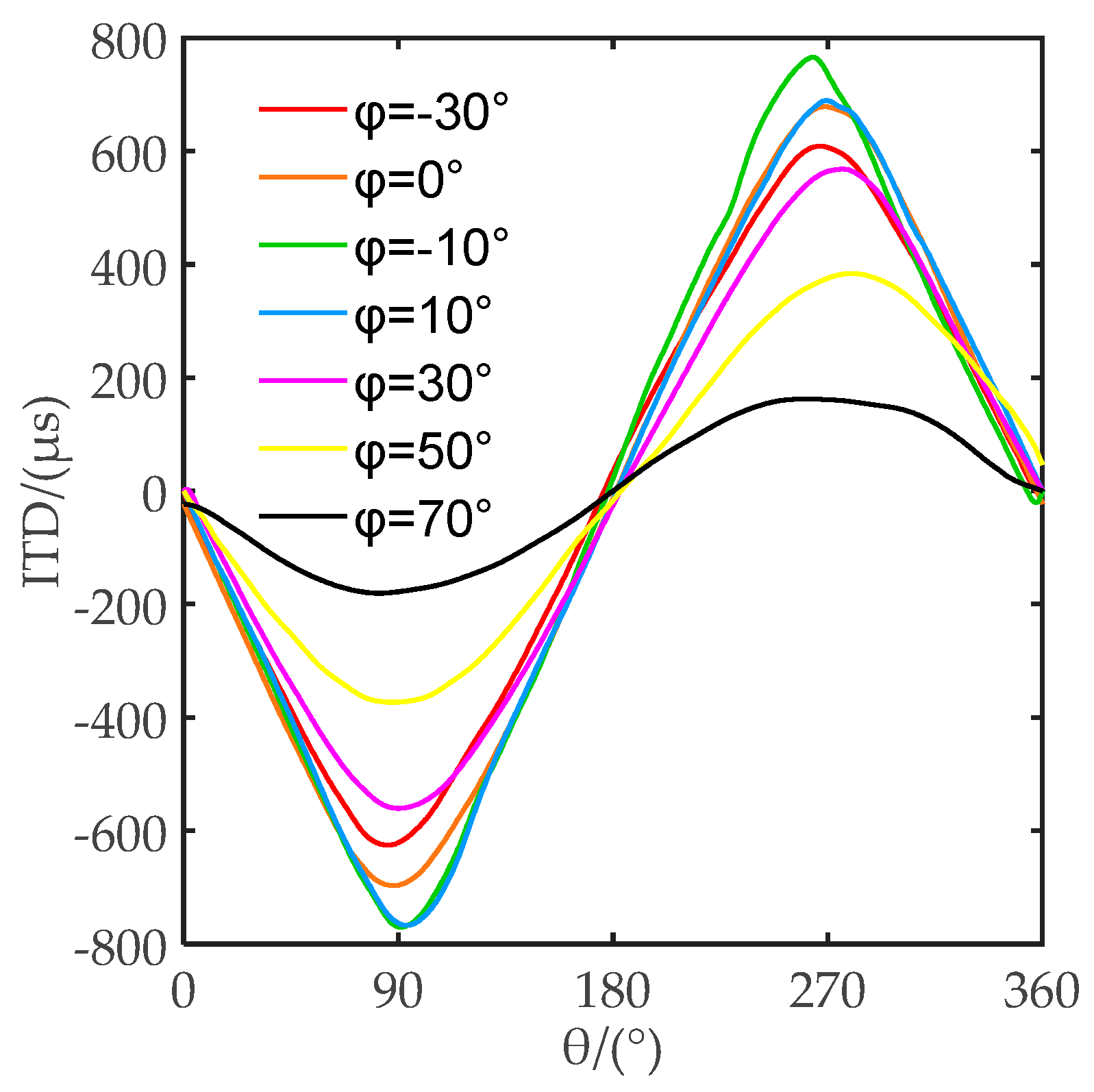
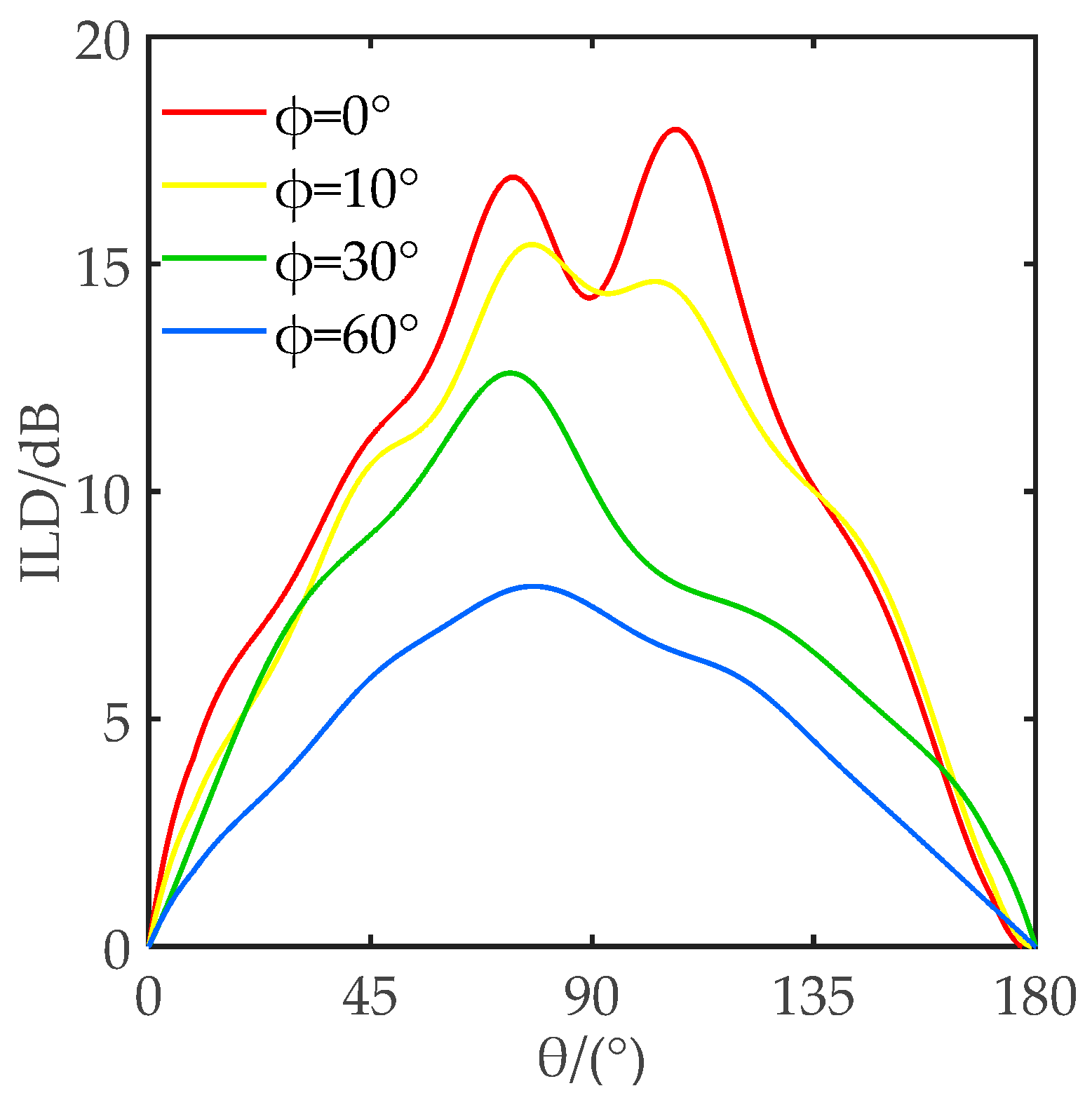
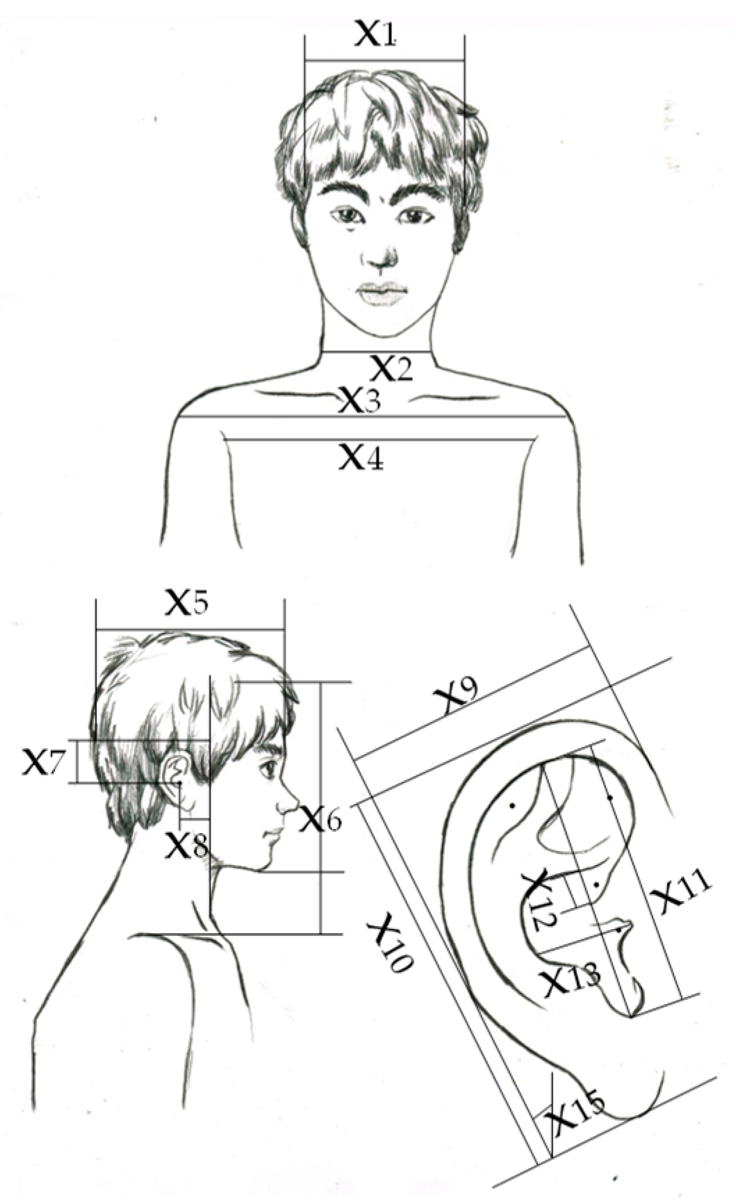
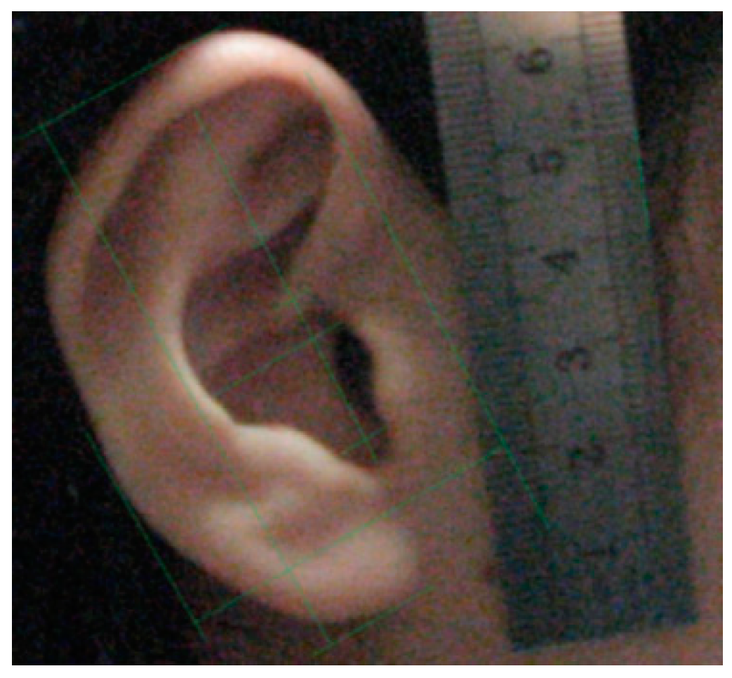
2.2. Characteristics Analysis

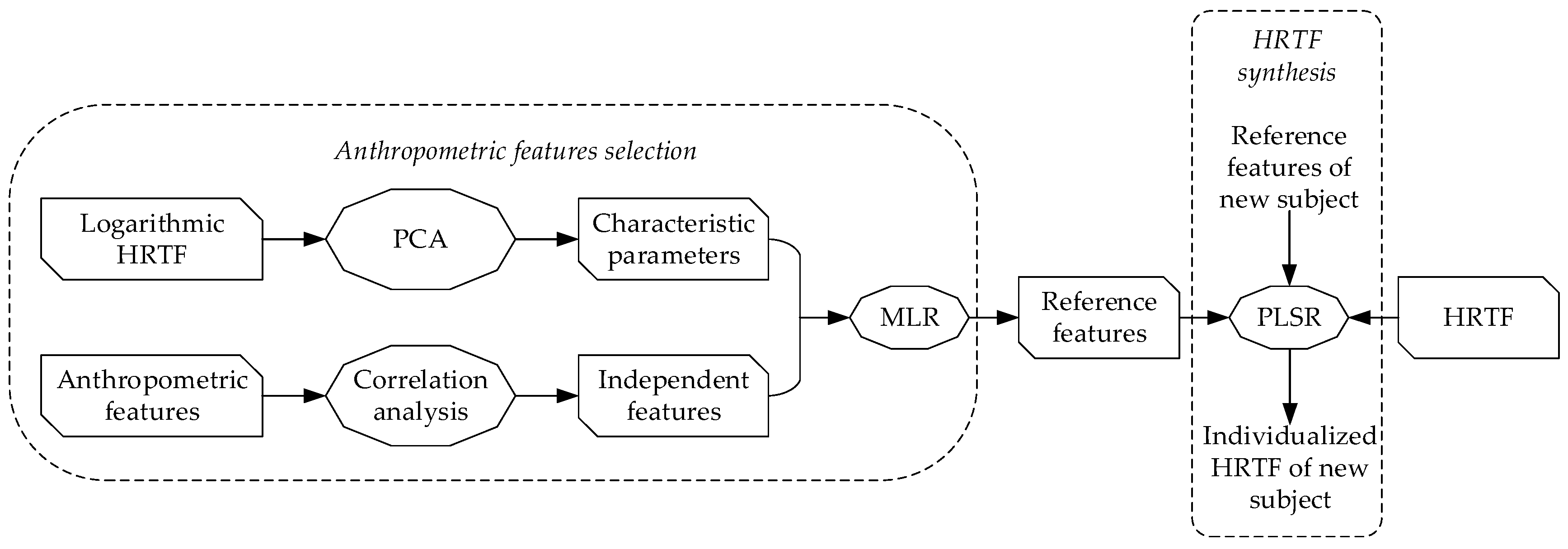
Interaural Time Difference (ITD) and Interaural Level Difference (ILD) are two important features that can be used to test the accuracy of HRTFs. Figure 1 shows the average value of ITD at different directions calculated from the HRTFs of 56 subjects in the database. Figure 2 shows the broadband average ILD (0~22.5 kHz) at different directions calculated from the HRTFs of 56 subjects in the database.

ITDs were calculated through the method of rising edge with 20% [18]. For a certain elevation, the ITDs at $0^{\circ }\le \theta \le {180}^{\circ }$ are symmetric to those at ${180}^{\circ }\le \theta \le {360}^{\circ }$. As sound moves laterally, the absolute value of ITD increases and reaches a maximum value near $\theta ={90}^{\circ }$ and $\theta ={270}^{\circ }$. Additionally, the elevation at horizontal plane has the largest ITD range, the ITD range decreases gradually as ϕ deviates from the horizontal plane. These results are consistent with existing literature [19].

As shown in Figure 2, ILDs are obviously asymmetric. The ILD generally has the largest variable range on the horizontal plane, which declines when the elevation increases. These are also consistent with the existing literature [18].

Furthermore, seven subjects were selected randomly to calculate their ITDs in the direction of θ = 0°, ϕ = 0° as shown in Figure 3. Although the ITDs of all the seven subjects perform the same tendency, there are still some apparent differences, such as the accurate location and value of the peak and valley, which also suggest the necessity of individualization for HRTFs.

3. Methodology

Since not all the anthropometric features in the database are related to human hearing, it is necessary to find out those closely related to HRTFs as reference features. Once they are found, the main focus in application is to measure them and use them to synthesize individualized HRTFs. The procedure for this algorithm is shown in Figure 4. First, PCA was used to extract the characteristic parameters of HRTFs. Then, MLR was conducted to find the relationship between HRTF characteristic parameters and anthropometric features. Next, PLSR was used to synthesize the phase and magnitude of HRTFs. Finally, the individualized HRTFs of a new subject were obtained.

3.1. Principle Component Analysis for HRTF Characteristics Parameters

Principle component analysis is a statistical technique for analyzing and simplifying data set. It is often used to reduce the dimensionality of a data set while retaining the features that contribute the most to the variance of the data set. In previous research [20,21,22], PCA had been proved of effective in reconstruction of HRTF logarithmic magnitude. In current research, we applied PCA on HRTF logarithmic magnitude to extract the principle components as the characteristic parameters.

The logarithmic magnitudes of HRTF at M directions on the horizontal plane can be denoted as:

$${[H_{\log }]}_{N\times M}=[\begin{array}{cc}{H}_{\log ,1}(f)& \begin{array}{cc}{H}_{\log ,2}(f)& \begin{array}{cc}\cdots & H_{\log ,M}(f)]\end{array}\end{array}\end{array}=\left[\begin{array}{cccc}{H}_{\log }({\theta }_1,f_1)& H_{\log }({\theta }_2,f_1)& \cdots & H_{\log }({\theta }_M,f_1)\\ H_{\log }({\theta }_1,f_2)& H_{\log }({\theta }_2,f_2)& \cdots & H_{\log }({\theta }_M,f_2)\\ ⋮& ⋮& \ddots & ⋮\\ H_{\log }({\theta }_1,f_N)& H_{\log }({\theta }_2,f_N)& \cdots & H_{\log }({\theta }_M,f_N)\end{array}\right]$$

(1)

where f = 1, 2, …, N denotes the frequency bin of HRTF. Then, the covariance matrix could be calculated as:

$${[R]}_{N\times N}=\frac{1}{M}{[H_{\log }]}_{N\times M}{[H_{\log }]}_{M\times N}^{+}$$

(2)

where [R] is an N by N Hermite matrix, and its eigenvalue is real. + denotes the generalized inverse of matrix [H_log]. Its eigenvector is extracted and arranged as the eigenvalue reduced-order $u_1,u_2,\dots ,u_Q$. Then the first Q eigenvectors are taken out as the base-vectors and to build a matrix:

$${[D]}_{N\times Q}=[u_1,u_2,\dots ,u_Q]$$

(3)

Because $u_1,u_2,\dots ,u_Q$ are orthogonal, ${[H_{\log }]}_{N\times M}$ can be decomposed on the use of these base-vectors, then the weight matrix can be achieved accordingly:

$${[W]}_{Q\times M}={[D]}_{Q\times N}^{+}{[H_{\log }]}_{N\times M}$$

(4)

herein, ${[W]}_{Q\times M}$ is the characteristic parameter of HRTFs. Figure 5 gives the result of PCA on a left ear’s HRTF logarithmic magnitudes. As can be seen, more than 95% accuracy of the HRTF logarithmic magnitudes can be reconstructed from six principle components.

3.2. Multiple Linear Regression for Anthropometric Feature Selection

In this research, multiple linear regression was used for selecting the anthropometric features closely relating to the HRTFs. Suppose the relationship between principle components and the corresponding anthropometric features in the spatial direction θ is:

$$w_{\theta }=X{B}_{\theta }+E_{\theta }$$

(5)

where $w_{\theta }$ represents the weight vector of HRTF logarithmic magnitude at direction $\theta$, $B_{\theta }$ represents the regression coefficients matrix, $X$ denotes the anthropometric feature matrix, $E_{\theta }$ represents the estimation error matrix, respectively. The regression coefficients matrix $B_{\theta }$ can be calculated through the anthropometric features:

$$B_{\theta }={(X^{T}X)}^{-1}{X}^T{w}_{\theta }$$

(6)

T represents the transpose of a matrix.

There were a number of anthropometric features in the database. For the reason that there were different correlations between the features and HRTFs, it was unnecessary to introduce all of them into the MLR models. By using unnecessary features, some useful information might be concealed, which led to a worse regression model. Meanwhile, getting rid of the unnecessary features alleviated the complexity of the system, which reduced the workload of the individualization procedure. In order to select the anthropometric features used in the regression model, correlation analysis was first conducted on different features. For the two features with large linear correlation coefficient, the one which had more significant influence was reserved. Then, correlation analysis was applied on the reserved features and HRTF logarithmic magnitudes to delete those features with smaller correlation coefficients. Next, the selected anthropometric features were introduced to the MLR model, in which F-test and backward selection at significant level α = 0.05 would be used to delete those insignificant features.

Considering the linear regression model:

$$Y=X\beta +\mathsf{\epsilon }$$

(7)

where $X$ is an n by p full rank matrix of known constant, $Y$ is an n-vector of response, $\beta$ is a p-vector of unknown parameter, and ε is an n by 1 unobservable error with a normal distribution N(0, σ²I_n). Assume that a hypothesis in model (7) is given by H₀: Aβ = c, where A is a known q by p matrix with rank q and c is a q by 1 vector. The usual test for hypothesis H₀ is F-test, which was equivalent to the likelihood ratio test. The test statistic F-statistic was given by:

$$F=\frac{1}{q{(\hat{\sigma })}^2}{(c-A\hat{\beta })}^T{[A{(X{X}^T)}^{-1}{A}^T]}^{-1}(c-A\hat{\beta })$$

(8)

where $\hat{\beta }={(X^{T}X)}^{-1}{X}^{T}Y$ is a least square estimation of $\beta$, and ${\sigma }^2=Y^T(I_n-P_x)Y/(n-p)$ is an unbiased estimator of σ² in model (7), where $P_x=X{(X^{T}X)}^{-1}{X}^T$. When H₀ holds the F-statistic Equation (8) distributes as an F distribution with degrees of freedom q and (n-p).

After the F-statistic has been calculated, the backward selection is used to select the significant features. First, all the features retained after correlation analysis were put into the regression model, then F-statistic of each feature was calculated and compared to the one at the significant level α = 0.05. After deleting the most insignificant feature, the rest ones were put into the model again and the insignificant one among them was deleted. This process was repeated until all the rest features were significant at the significant level α = 0.05.

Table 2. Anthropometric features retained after each processing procedure.

Processing Procedure	Anthropometric Features Retained
Correlation analysis between different anthropometric parameters	x1, x2, x3, x4, x5, x6, x7, x8, x9, x10, x11, x12, x13, x14, x15
Correlation analysis between weight vector and remaining anthropometric parameters	x1, x2, x3, x4, x5, x6, x7, x8, x10, x12, x13, x14
Multiple linear regression	x1, x2, x3, x4, x5, x6, x7, x8, x10, x12, x14

gives the results of anthropometric feature selection for each step. And the anthropometric features are shown in detail as Figure 6.

Thus far, the anthropometric features retained were used as the reference features in the following HRTF synthesis.

3.3. Partial Least Square Regression for HRTF Synthesis

Partial least square regression is a statistical method that is used to search the basic functional relationship between two matrices [23]. It is often used in mapping the linear relationship from multiple independent variables to multiple dependent variables.

Assuming that the optimized anthropometric features of S subjects and the logarithmic magnitudes of HRTFs at M directions are presented with the matrices:

$$\begin{gathered} X_{F\times S}=\left[\begin{array}{cccc}{x}_{11}& x_{12}& \cdots & x_{1S}\\ x_{21}& x_{22}& \cdots & x_{2S}\\ ⋮& ⋮& \ddots & ⋮\\ x_{F1}& x_{F2}& \cdots & x_{FS}\end{array}\right] \\ {[H_{\log ,f}]}_{M\times S\times N}=\left[\begin{array}{cccc}{H}_{\log ,f}({\theta }_1,S_1)& H_{\log ,f}({\theta }_1,S_2)& \cdots & H_{\log ,f}({\theta }_1,S_S)\\ H_{\log ,f}({\theta }_2,S_1)& H_{\log ,f}({\theta }_2,S_2)& \cdots & H_{\log ,f}({\theta }_2,S_S)\\ ⋮& ⋮& \ddots & ⋮\\ H_{\log ,f}({\theta }_M,S_1)& H_{\log ,f}({\theta }_M,S_2)& \cdots & H_{\log ,f}({\theta }_M,S_S)\end{array}\right] \end{gathered}$$

(9)

where F, S, M and N represent the number of anthropometric features used in the model, training subjects, training azimuths and the frequency bins of HRTF, respectively.

The first step of PLSR is to normalize the dependent and independent matrices. The normalization process is conducted as the equation below:

$$a_{ij}^{*}=\frac{a_{ij}-m_{ij}}{M_{ij}-m_{ij}}$$

(10)

where $a_{ij}^{*}$ stands for the normalized value of $a_{ij}$, $M_{ij}$ and $m_{ij}$ stand for the maximum and minimum value of $a_{ij}$, respectively. The normalized matrices are $X_0$ and $H_0$.

The second step is to construct the internal and external relationships between dependent variables and independent variables, and implement the regression of $X_0$ and $H_0$ on the first component:

$$X_0=t_1{p}_1^T+X_1$$

(11)

$$H_0=t_1{r}_1^T+H_1$$

(12)

where $t_1$ represents the first component extracted from $X_0$, $p_1$ and $r_1$ represent the regression coefficients, $H_1$ and $X_1$ represent the residual of $X_0$ and $H_0$, respectively.

Next, $X_0$ and $H_0$ are replaced with $X_1$ and $H_1$, and the second step is repeated for l times until the accuracy of regression equation met the requirement, where l is determined by the cross validation seeing [22]. Then, the estimation of $H_0$ can be denoted as:

$${\hat{H}}_0={\displaystyle \sum _{i=1}^l{\mathrm{t}}_i{\mathrm{r}}_i^T}$$

(13)

Finally, according to the inverse process of normalization, the regression equation can be restored. Figure 7 shows an example data of measured and synthesized HRTF on the left ear of a KEMAR dummy head at θ = 0° on the horizontal plane.

4. Experimental Investigations

4.1. Objective Experiments

To evaluate the performance of the presented HRTF individualization method, the leave-one-out cross validation approach was used [24]. Each subject in the database was taken out successively as the testing subject with the remaining 55 ones being used for training.

The spectral distortion was used as the objective evaluation metric. The results of the presented HRTF individualization method was compared with other two existed HRTF individualization methods, which had been verified to be effective previously. One was database-matching approach proposed in [7], the other was general regression neural network based method presented in [25].

4.1.1. Evaluation Criteria

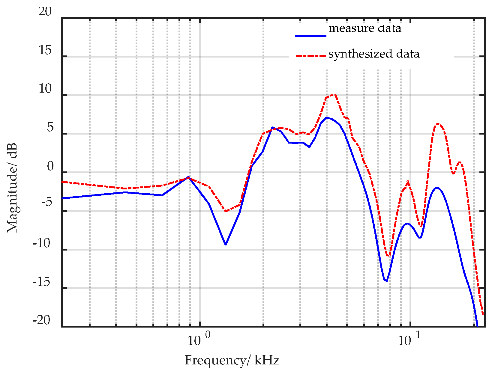
The error metric of spectral distortion widely used was employed to evaluate the synthesis precision of the individualized HRTFs:

$$S{D}^{(d)}=\sqrt{\frac{1}{K}{\displaystyle \sum _{k=1}^K{(20{\log }_{10}\frac{\Vert H^{(d)}{}_k\Vert }{\Vert {\hat{H}}^{(d)}{}_k\Vert })}^2}}$$

(14)

where $H^{(d)}{}_k$ is the measured HRTF at d-th direction, ${\stackrel{\wedge }{H}}^{(d)}{}_k$ is the synthesized HRTF at the same direction, and k is the number of the frequency bin (K = 400).

Then, the root-mean-square error (RMSE) was used to compare the two sets of HRTFs at all the 72 directions on the horizontal plane:

$$SD(H,\hat{H})=\sqrt{\frac{1}{D}{\displaystyle \sum _{d=1}^D{[S{D}^{(d)}(H,\hat{H})]}^2}}$$

(15)

where D stand for the direction of HRTF, D = 72.

4.1.2. Results

The results of the objective evaluation experiments are presented in

Table 3. Average spectral distortion between the synthesized and the measured HRTF (dB).

Individualization Method	Left Ear	Right Ear	Average
Proposed method	7.2537	6.9303	7.0920
GRNN based method	7.7385	7.1026	7.4206
Database-matching method	7.8314	8.2359	8.0337

, which validates the feasibility of the presented HRTF individualization method. The presented method achieved small synthesis error when compared with both the database matching one and general regression neural network (GRNN) base method. It is also notable that the proposed method achieved balanced synthesis errors for left and right ears, while the other two methods achieved relatively larger synthesis errors for left ear and smaller errors for right ear. Consequently, the proposed method was proved to be algorithmically effective and embodies the superiority in the balanced synthesis error of left and right ear.

4.2. Subjective Experiments for Discrimination Degree of Given Azimuths

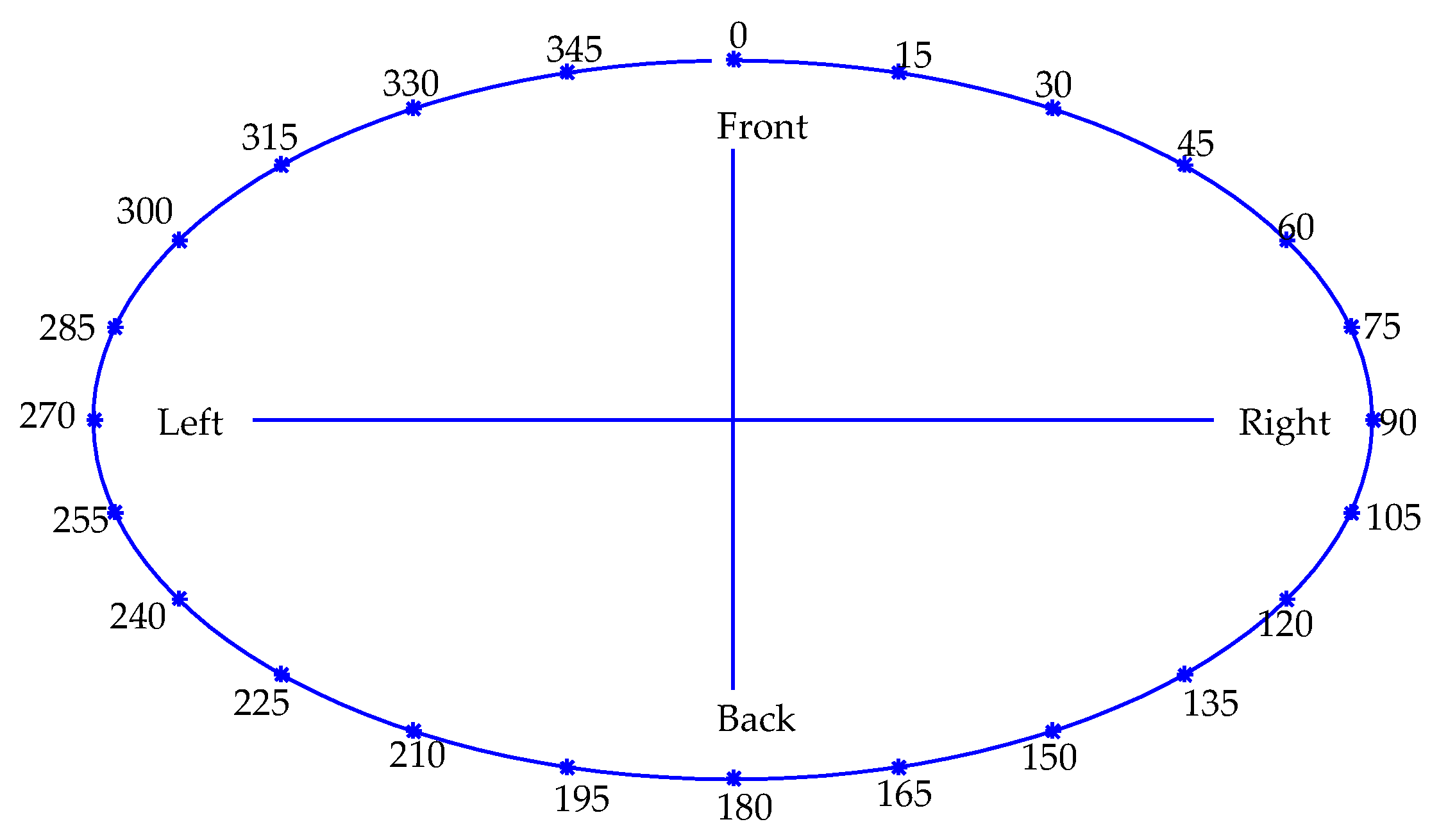
4.2.1. Experimental Protocols

To investigate the effectiveness and superiority of the individualized HRTFs in perceiving the spatialization cues, a subjective experiment was conducted to compare the directional discrimination degree of sound sources. This experiment tested two HRTF species: individualized HRTFs (obtained from the presented method) and non-individualized ones (measured from KEMAR dummy head). Eight Chinese adults (four males and four females) aged between 23 and 27 were employed. They were postgraduates and doctoral student majoring in acoustics with self-reported normal hearing and former subjective experiment experience. All the participants were remunerated for their participation. Prior to the experiment, the reference features selected in Section 3.2 of each participant were measured to synthesize their individualized HRTFs. For body features of x₁, x₂, x₃, x₄, x₅, x₆, x₇, x₈ and x₁₄, they were measured directly by a ruler, for head and ear features of x₉, x₁₀, x₁₁, x₁₂, x₁₃, they were measured from digital photographs as shown in Figure 8. On the basis of Inverse Fast Fourier Transform, HRTFs were transferred into HRIRs. Then testing stimuli were produced by convolving the HRIRs with an original double-channel notify signal whose waveform in time domain is shown in Figure 9. The testing stimuli were presented to the participants through Hi-Fi headphone [Sennheiser HD560].

4.2.2. Procedure

In this experiment, the semantic differential method [26,27,28] was adopted to evaluate the directional discrimination degree of sound sources. The order scale was used for evaluation, in which directional discrimination degrees are shown as

Table 4. Directional discrimination degree class.

Discrimination Degree	Unconspicuous	Detectable	Obvious	Very Obvious	Extremely Obvious
Class	1	2	3	4	5

. Before the experiment, the instructions and the questionnaires were handed out to the participants. On the questionnaire, the azimuth information of each testing stimulus was listed. During the experiment, each stimulus was played five times in succession, and then there would be a 5 s interval for the participants to select a class (listed in Table 4) according to their judgments. Then, the next stimulus would be presented in the same way until all the stimuli are played. There were totally 24 testing azimuths as shown in Figure 10. As a result, there were 24 (testing azimuth) × 2 (HRTF species) × 8 (participants) = 384 testing stimuli in total, and there were 24 × 2 = 48 testing stimuli for each participant.

In the experiment, the testing stimuli were divided into two groups (stimuli with individualized HRTFs and stimuli with non-individualized ones) based on the HRTF species, but the participants were unaware of this. The presentation order of testing stimuli in each group was randomized by the Latin square scheme to minimize the deviation of the experimental results that might be caused by the test sequence. This psychoacoustic experiment was performed only once, and the subjects were required to make only one judgment for each stimulus. The experiment took about 15 min for each participant.

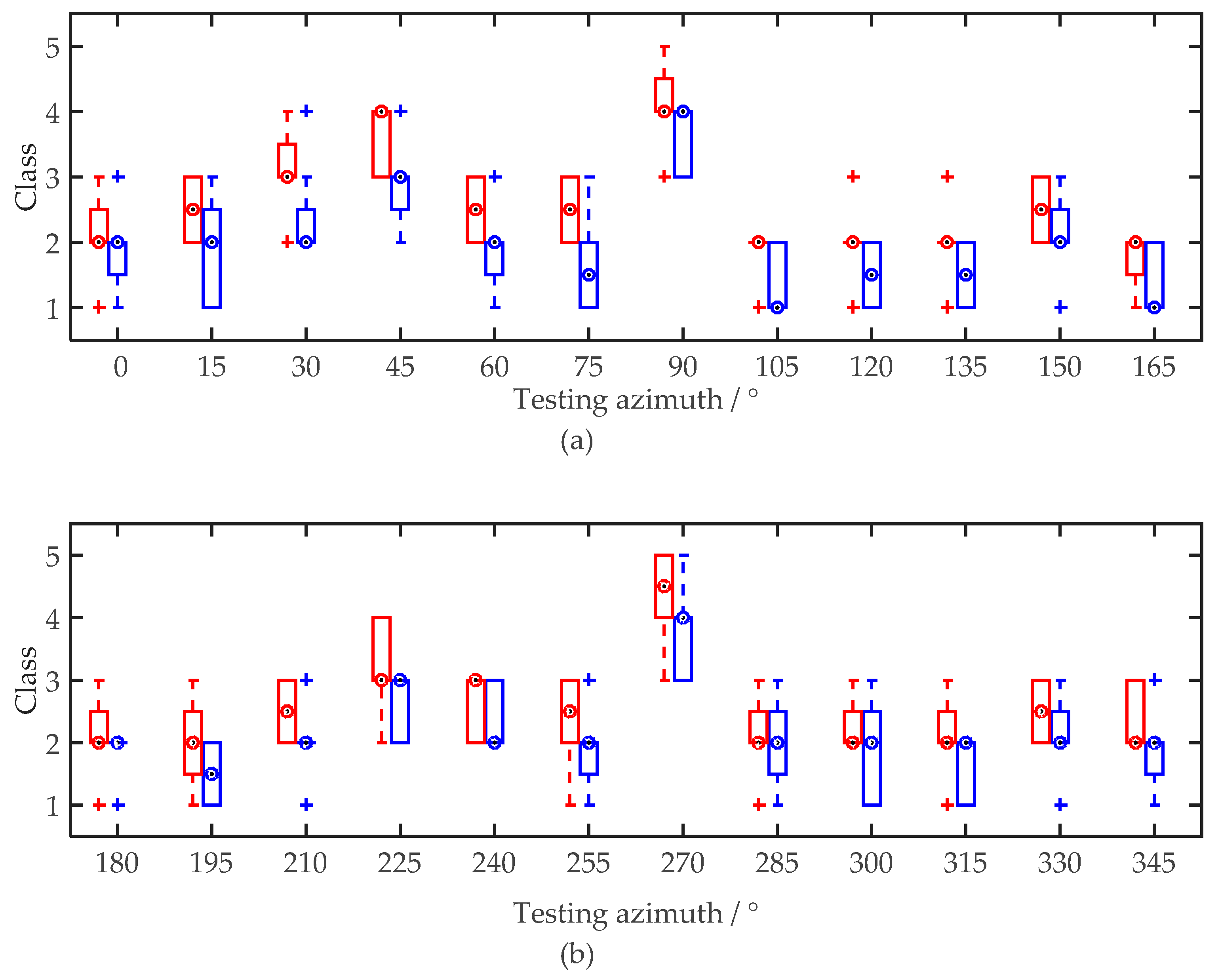
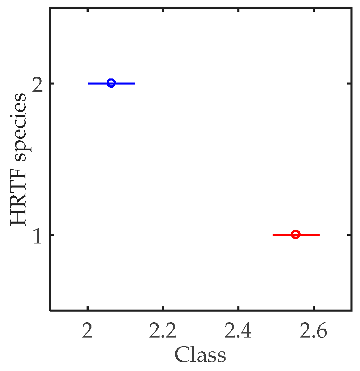
4.2.3. Results and Analysis

Figure 11 gives the results of the subjective experiment for discrimination degree of given azimuths, in which an upper and shorter box implies a better evaluation results. As shown in Figure 11, stimuli with individualized HRTFs are evidently easy to discriminate the azimuth information. Despite that the stimuli at directions of 90° and 270° are easy to discriminate with non-individualized HRTFs, the individualized ones even improve the discrimination degree. At azimuths of 30° and 45°, the performance of the individualized HRTF species is obviously superior to the non-individualized species in the 25th percentiles, the median and the 75th percentiles. Moreover, the stimuli with azimuths in front of the listening subject (left part of Figure 11a and right part of Figure 11b) are noted easy to discriminate than the ones at the back of the listener (right part of Figure 11a and left part of Figure 11a). This is caused by the human auditory nature of being sensitive to the front directions.

To determine whether the individualized HRTFs perform better than the non-individualized ones in this subjective experiment, statistical analysis was made. First of all, a two-way repeated variance analysis (ANOVA) was made under the significance level of α = 0.05 to verify the validity of the experimental results. It was hypothesized that both the testing HRTF species and azimuths had no significant effect on the subjects (H₀). The hypothesis was kept if p was larger than α (p stands for the probability of making mistakes regarding to rejecting H₀). The hypothesis was rejected if p was less than α, the factor was thus considered to have significant effect on the subjects. The result of ANOVA was shown in

Table 5. Result of two-way repeated variance analysis.

Item	HRTF Species	Azimuth	Interaction
F	62.7302	18.3263	0.3395
p	0	0	0.9984
H0	Rejected	Rejected	Kept

. As can be seen from Table 5, both the HRTF species and the testing azimuth had significant effect on the participants, while the interaction of HRTF species and azimuth had no significant effect on the participants. Consequently, the psychoacoustic experiment was considered to be valid.

Next, the Least Significant Difference (LSD) for independent samples was employed as the post-hoc of ANOVA to determine whether the individualized HRTFs performed better than the non-individualized ones in this experiment. It was hypothesized that there was no significant difference between the evaluation results of individualized HRTFs and non-individualized ones (H₀). p stands for the probability of making mistakes regarding to rejecting H₀. H₀ was kept when p was larger than α, while H₀ was rejected when p was less than α. Under the significant level of α = 0.05, the result of LSD was given in

Table 6. Post-hoc for ANOVA. Mean_ind and mean_non denote the mean classes of the individualized HRTFs and the non-individualized ones, respectively.

p	H0	Mean_ind	Mean_non
0	Rejected	2.5521	2.0625

and Figure 12. As can be seen from Table 6, the evaluation results were significantly different between individualized HRTFs and the non-individualized ones. The mean class of the individualized HRTFs was larger than that of the non-individualized ones. The individualized HRTFs were consequently considered performing better than the non-individualized ones in this psychoacoustic experiment.

The results of this subjective experiment indicate that, comparing with the non-individualized HRTFs, the individualized ones obtained from the presented integrated method involved more accurate directional information. Meanwhile, the individual HRTFs performed better in discriminating the directional information. This is of great significance in the practical application.

4.3. Subjective Experiment for Auditory Localization

4.3.1. Experimental Protocols

The experiment in Section 4.2 indicated that the directional information of sound sources with individualized HRTFs were easier to be detected when the azimuth had been known before. To further verify the superiority of the individualized HRTFs in perceiving the spatialization cues when the directional information was unknown for the listeners, the subjective localization experiment was also carried in this section. The participants employed in this experiment were the same as Section 4.2. The localization experiment also tested two HRTF species: individualized HRTFs (obtained from the presented method) and non-individualized HRTFs (measured from KEMAR dummy head). There were totally 22 testing azimuths on the horizontal plane. The testing stimuli were produced by convolving the signal shown in Figure 8 with the HRIRs of the testing azimuths. The testing azimuths were: 0°, 15°, 30°, 45°, 65°, 80°, 100°, 115°, 135°, 150°, 165°, 180°, 195°, 210°, 225°, 245°, 260°, 280°, 295°, 315°, 330° and 345°. 0° denotes the front of the subject, and the azimuth increases clockwise.

4.3.2. Procedure

During the experiment, the testing stimuli were presented to the participants directly through headphones [Sennheiser HD 560]. Before the test, the instructions and questionnaires for the experiment were handed out to all the participants. On the questionnaire, all the testing azimuths were listed for each testing stimulus. The participants were asked to select the most accurate azimuth according to their own judgments after hearing the stimulus. During the test, each stimulus was presented five times in succession. Then, there would be a 5 s interval, in which the participants made their judgments to the presented stimulus on the questionnaire. After that, the next stimulus would be presented in the same way, until all the testing stimuli of the two testing HRTF species were finished. The test continued until this process was repeated three times. To avoid the possible bias of the localization results caused by auditory fatigue, there was a 20 min rest between repetitions.

The presentation order of the stimuli was randomized using an altered Latin square scheme. Thus, the possible bias effects caused by the order effect and sequential dependencies could be minimized. The auditory localization experiment lasted about 1.5 h for each participant.

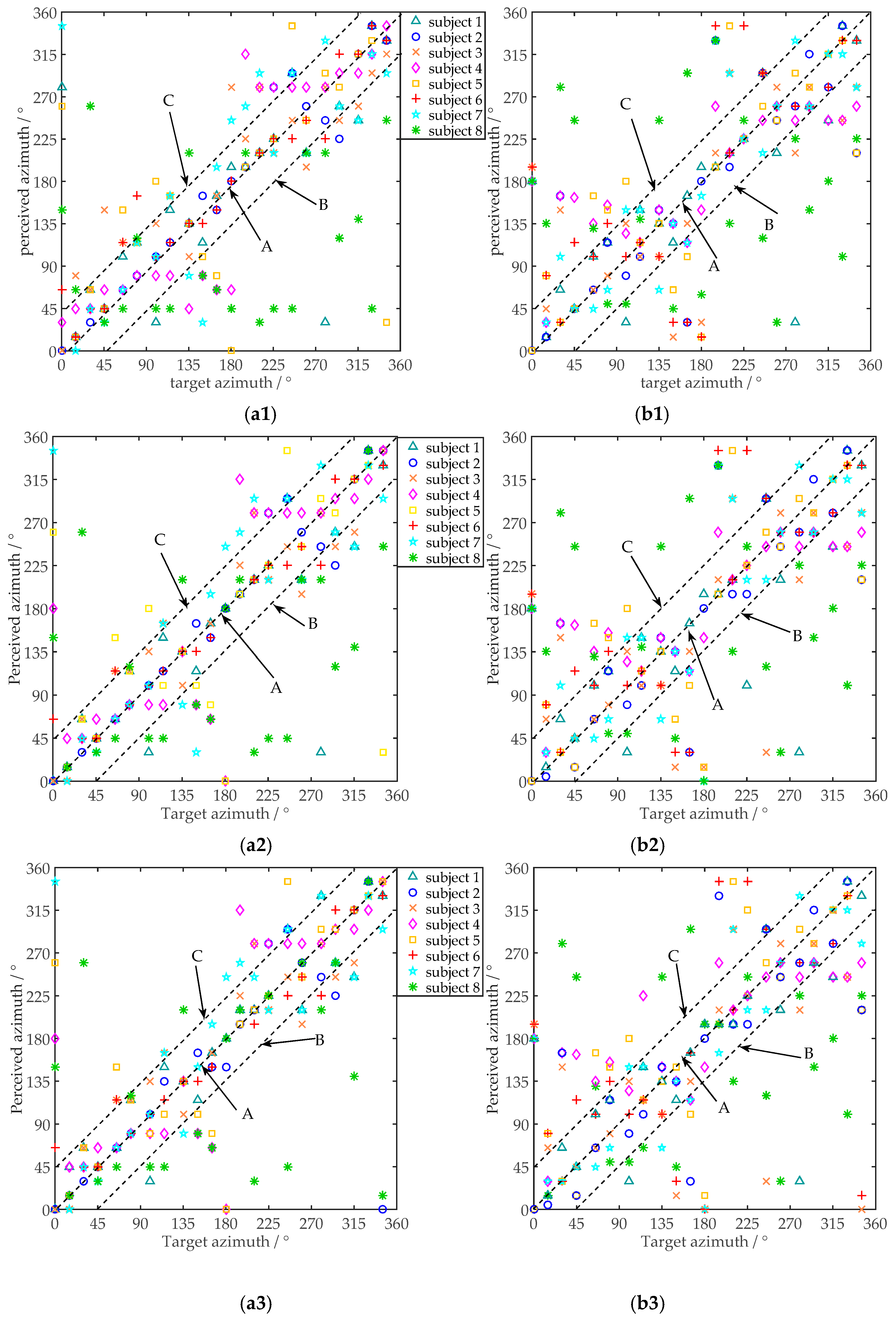
4.3.3. Results and Analysis

Figure 13 shows the localization results of all the eight subjects by using the presented individualized HRTFs and the non-individualized ones of KEMAR dummy head. X-axis and Y-axis stand for the real azimuth and the perceived azimuth, respectively. Perfect correlation between target azimuth and response judgment corresponds points on line A on these graphs. That means the subjects’ judgments were exactly the same as the real directions. On the other hand, points out of line B and line C correspond to localization errors larger than 45°. Besides, points on the coordinate line of 180° correspond to front-back confusions. It can be observed that the individualized HRTFs achieve slightly better localization performance, both in accurate localization and smaller localization error.

As a supplementary to the data shown in Figure 13, the localization accuracy rate, the average error angle and mean of the standard deviation of the error were calculated, and the results are listed in

Table 7. Statistical results of the localization experiment.

HRTF Species	Item	Subject 1	Subject 2	Subject 3	Subject 4	Subject 5	Subject 6	Subject 7	Subject 8
Individualized HRTF	Accuracy rate/(%)	39.3	62.1	30.3	25.8	39.4	42.4	16.7	12.1
	Average error/(°)	26.97	12.80	32.58	42.88	37.88	15.83	28.71	81.71
	Standard deviation/(°)	30.86	20.97	29.79	38.56	47.51	23.98	29.59	56.55
General HRTF	Accuracy rate/(%)	28.8	18.2	24.2	21.2	37.9	28.2	16.7	3.0
	Average error/(°)	37.8	38.94	53.94	51.80	44.62	56.21	46.21	80.76
	Standard deviation/(°)	43.27	49.08	50.96	49.04	53.30	57.23	45.31	52.16

.

It can be found from Table 7 that the localization accuracy rates of the individualized HRTFs were larger than those of non-individualized ones, except subject 7. The average localization errors of the individualized HRTFs were smaller than the non-individualized ones for all the participants, even though the difference was not obvious for subject 8. Moreover, the standard deviations of the individualized HRTFs were smaller than the non-individualized ones for participants, except subject 8. The individualized HRTFs seemed to be preferable in auditory localization.

To determine whether the experimental results were valid, two-way repeated variance analysis (ANOVA) was made for the localization errors of each subject under the significant level of α = 0.05. The two factors were HRTF species and testing azimuth. It was hypothesized that both the HRTF species and testing azimuth had no significant effect on the localization errors (H₀). p denotes the probability of making mistakes regarding to rejecting H₀. H₀ was kept when the probability p was larger than α, while H₀ was rejected when p was less than α. The result of ANOVA was listed in

Table 8. The result of two-way repeated analysis of variance.

Item	HRTF Species	Azimuth	Interaction
F	41.4313	7.4317	2.6415
p	0	0	0
H0	Rejected	Rejected	Rejected

. As can be seen from Table 8, the HRTF species, testing azimuth and their interaction had significant effect on the localization errors. Consequently, the localization experiment was proved valid.

Next, the Least Significant Difference (LSD) for independent samples was employed as the post-hoc of ANOVA to determine whether the individualized HRTFs performed better than the non-individualized ones in the binaural localization experiment. The localization errors of the testing HRTF species were hypothesized to be of no significant difference (H₀). p stands for the probability of making mistakes regarding to rejecting H₀. H₀ was kept when p was larger than α while H₀ was rejected when p was less than α. Under the significance level of α = 0.05, the result of the post-hoc was shown in

Table 9. Post-hoc for two-way repeated ANOVA. Mean_ind and mean_non denote the mean localization errors of the individualized HRTFs and the non-individualized ones, respectively.

p	H0	Mean_ind	Mean_non
0	Rejected	35.9091	53.7860

and Figure 14.

It can be found from Table 9 that under the significant level of α = 0.05, the localization errors of the individualized HRTFs and the non-individualized ones are significantly different. For the reason that the mean localization error of the individualized HRTFs was less than that of the non-individualized ones, the individualized HRTFs were considered performing better than the non-individualized ones in the binaural localization experiment.

5. Conclusions

The main contributions of this research lie in: (1) an integrated algorithm for HRTF individualization combining correlation analysis, principle component analysis, multiple linear regressions and partial least square regression was presented; (2) two psychoacoustic experiments were conducted to explore the superiority of the individualized HRTFs in perceiving the spatialization cues of sound sources. All the results support that the individualized HRTFs obtained through the presented integrated method achieve preferable performance in perceiving the spatialization cues than the general non-individualized ones.

Given the conclusions above, individualized HRTFs should be more necessary in practical applications, such as virtual hearing, tel-conference, etc. However, the practical applications involve not only spatialization cues, but also other attributes such as timbre. The use of HRTFs or even individualized HRTFs may possibly cause some other good or bad effects, which were not considered in this research. Thus, future work will need to investigate whether HRTFs and individualized HRTFs leads to some potential effects on binaural auditory in practical applications.

References

1. Blauert, J.P. Spatial Hearing; Revised Edition; MIT: Cambridge, MA, USA, 1997. [Google Scholar]
2. Algazi, V.R.; Duda, R.O.; Duraiswami, R.; Gumerov, N.A.; Tang, Z. Approximating the head-related transfer function using simple geometric models of the head and torso. J. Acoust. Soc. Am. 2002, 112, 2053–2064. [Google Scholar] [CrossRef] [PubMed]
3. Katz, B.F. Boundary element method calculation of individual head-related transfer function. I. Rigid model calculation. J. Acoust. Soc. Am. 2001, 110, 2440–2448. [Google Scholar] [CrossRef] [PubMed]
4. Meshram, A.; Mehra, R.; Yang, H.; Dunn, E.; Franm, J.M.; Manocha, D. P-HRTF: Efficient personalized HRTF computation for high-fidelity spatial sound. In Proceedings of the IEEE International Symposium on Mixed and Augmented Reality (ISMAR), Munich, Germany, 10–12 September 2014. [Google Scholar]
5. Zeng, X.Y. Customization Methods of Head-related Transfer Function. Audio Eng. 2007, 31, 41–46. [Google Scholar] [CrossRef]
6. Zotkin, D.N.; Hwang, J.; Duraiswami, R.; Davis, L.S. HRTF personalization using anthropometric measurements. In Proceedings of the IEEE Workshop on Applications of Signal Processing to Audio and Acoustics, New Paltz, NY, USA, 19‒22 October 2003; pp. 157–160. [Google Scholar] [CrossRef]
7. Zeng, X.Y.; Wang, S.G.; Gao, L.P. A hybrid algorithm for selecting head-related transfer function based on similarity of anthropometric structures. J. Sound Vib. 2010, 329, 4093–4106. [Google Scholar] [CrossRef]
8. Andreopoulou, A.; Roginska, A. Database Matching of Sparsely Measured Head-Related Transfer Functions. J. Audio Eng. Soc. 2017, 65, 552–561. [Google Scholar] [CrossRef]
9. Nishino, T.; Inoue, N.; Takeda, K.; Itakura, F. Estimation of HRTFs on the horizontal plane using physical features. J. Acoust. Soc. Am. 2007, 68, 897–908. [Google Scholar] [CrossRef]
10. Tang, Y.; Fang, Y.; Huang, Q. Audio personalization using head related transfer function in 3DTV. In Proceedings of the 3dtv Conference: The True Vision-Capture, Antalya, Turkey, 16–18 May 2011; pp. 1–4. [Google Scholar] [CrossRef]
11. Hu, H.; Zhou, L.; Ma, H.; Wu, Z. HRTF personalization based on artificial neural network in individual virtual auditory space. J. Appl. Acoust. 2008, 69, 163–172. [Google Scholar] [CrossRef]
12. Bilinski, P.T.; Ahrens, J.; Thomas, M.R.; Tashev, I.; Platt, J. HRTF magnitude synthesis via sparse representation of anthropometric features. In Proceedings of the International Conference on Acoustics, Speech, and Signal Processing, Florence, Italy, 4–9 May 2014; pp. 4468–4472. [Google Scholar] [CrossRef]
13. Tashev, I. HRTF phase synthesis via sparse representation of anthropometric features. In Proceedings of the Information Theory and Applications Workshop (ITA), San Diego, CA, USA, 9–14 February 2014; pp. 1–5. [Google Scholar] [CrossRef]
14. He, J.; Gan, W.; Tan, E. On the preprocessing and postprocessing of HRTF individualization based on sparse representation of anthropometric features. In Proceedings of the IEEE International Conference on Acoustics, Speech and Signal Processing (ICASSP), Brisbane, Australia, 19–24 April 2015; pp. 639–643. [Google Scholar]
15. Zhu, M.; Shahnawaz, M.; Tubaro, S.; Sarti, A. HRTF personalization based on weighted sparse representation of anthropometric features. In Proceedings of the International Conference on 3D Immersion (IC3D), Brussels, Belgium, 11–12 December 2017. [Google Scholar] [CrossRef]
16. Spagnol, S.; Geronazzo, M.; Avanzini, F. On the relation between pinna reflection patterns and head-related transfer function features. IEEE Trans. Audio Speech Lang. Process. 2013, 21, 508–519. [Google Scholar] [CrossRef]
17. Hugeng, W.W.; Dadang, G. Improved Method for individualization of Head-Related Transfer Functions on Horizontal Plane Using Reduced Number of Anthropometric Measurements. J. Telecommun. 2010, 2, 31–41. [Google Scholar]
18. Xie, B.S.; Zhong, X.L.; Rao, D. Head-Related transfer function database and its analysis. Sci. China Ser. G Phys. Mech. Astron. 2007, 50, 267–280. [Google Scholar] [CrossRef]
19. Gardner, W.G. 3-D Audio Using Loudspeakers. Ph.D. Thesis, Massachusetts Institute of Technology, Cambridge, MA, USA, 1997. [Google Scholar]
20. Martens, W.L. Principal components analysis and resynthesis of spectral cues to perceived direction. In Proceedings of the 1987 International Computer Music Conference, San Francisco, CA, USA, 1987; pp. 274–281. [Google Scholar]
21. Kistler, D.J.; Wightman, F.L. A model of head-related transfer functions based on principal components analysis and minimum-phase reconstruction. J. Acoust. Soc. Am. 1992, 91, 1637–1647. [Google Scholar] [CrossRef] [PubMed]
22. Middlebrooks, J.C.; Green, D.M. Observations on a principal components analysis of head-related transfer functions. J. Acoust. Soc. Am. 1992, 92, 597–599. [Google Scholar] [CrossRef] [PubMed]
23. Hoskuldsson, A. PLS regression methods. J. Chemom. 1988, 2, 211–228. [Google Scholar] [CrossRef]
24. Hastie, T.; Tibshirani, R.; Friedman, J. The Elements of Statistical Learning: Data Mining, Inference, and Prediction, 2nd ed.; Springer: Berlin, Germany, 2009. [Google Scholar]
25. Wang, L.; Zeng, X.Y. New method for synthesizing personalized Head-Related Transfer Function. In Proceedings of the IEEE International Workshop on Acoustic Signal Enhancement (IWAENC), Xi’an, China, 13–16 September 2016. [Google Scholar]
26. Huang, H.B.; Huang, X.R.; Li, R.X.; Lim, T.C.; Ding, W.P. Sound quality prediction of vehicle interior noise using deep belief networks. Appl. Acoust. 2016, 113, 149–161. [Google Scholar] [CrossRef]
27. Wang, Y.S.; Shen, G.Q.; Xing, Y.F. A sound quality model for objective synthesis evaluation of vehicle interior noise based on artificial neural network. Mech. Syst. Signal Process. 2014, 45, 255–266. [Google Scholar] [CrossRef]
28. Han, L.; Kean, C.; Xue, W.; Yan, G.; Weiwei, Y. A perceptual dissimilarities based nonlinear sound quality model for range hood noise. J. Acoust. Soc. Am. 2018, 144, 2300–2311. [Google Scholar] [CrossRef]
Figure 1. Average Interaural Time Difference (ITD) value of 56 subjects at different directions. The X-axis stands for the azimuths of sound source, and the Y-axis stands for the ITD value. Curves in different colors represent the ITD variation trends of sound sources with different elevations.
Applsci 09 01867 g001
Figure 2. Broadband average Interaural Level Difference (ILD) (0~22.5 kHz) at different directions in audible band of 56 subjects. X-axis and Y-axis denote the azimuth and ILD value of sound source, respectively. Curves in different color represent the ILD variation trend of sound sources with different elevations.
Applsci 09 01867 g002
Figure 3. ITD contrast of different subjects in a same direction. X-axis denotes the azimuth of the sound source, Y-axis denotes the ITD value, and curves in different color denote the ITD variation trends of different subjects.
Applsci 09 01867 g003
Figure 4. Schematic diagram of the integrated head-related transfer functions (HRTF) individualization method. MLR: Multiple Linear Regression; PCA: Principle Component Analysis.
Applsci 09 01867 g004
Figure 5. Result of PCA on a left ear’s HRTF logarithmic magnitudes.
Applsci 09 01867 g005
Figure 6. The anthropometric features used in the presented integrated method. x14 is the seated height, which is not marked in the figure.
Applsci 09 01867 g006
Figure 7. The comparison of measure data and synthesized data for KEMAR dummy head at same direction. The solid line in blue represents the measured data of HRTF, and the broken line in red represent the synthesized data of HRTF, respectively.
Applsci 09 01867 g007
Figure 8. Measurement sketch for ear and head features.
Applsci 09 01867 g008
Figure 9. The waveform of original notify signal in time domain, the orange curve and blue curve stand for the data in different channels, respectively.
Applsci 09 01867 g009
Figure 10. Testing azimuths in the experiment for Discrimination Degree of Given Azimuths.
Applsci 09 01867 g010
Figure 11. Box-plot for results of the subjective experiment for discrimination degree of given azimuths. (a) and (b) represent the azimuths in right and left of the subject, respectively. X-axis and Y-axis denote the testing azimuths and the discrimination degree showed in Table 4, respectively. Red and blue boxes denote the HRTF species of the presented individualization method and KEMAR dummy head. Box edges mark the 25th and 75th percentiles, black dots in a circle mark the median. Outliers are indicated by +.
Applsci 09 01867 g011
Figure 12. The result of post-hoc for ANOVA. X-axis denotes the evaluation class. Y-axis denotes the testing HRTF species of (1) individualized HRTFs and (2) non-individualized HRTFs. Red and blue lines denote the HRTF species of individualized one and non-individualized one, respectively. Circles on the lines denote the mean class of the corresponding HRTF species. The lengths of the lines denote the mean confidence intervals of the corresponding HRTF species.
Applsci 09 01867 g012
Figure 13. Results of the subjective localization experiments, (a1a3) denote the results of the three repetitions for the presented individualized HRTFs, (b1b3) denote the results of the three repetitions for non-individualized HRTFs. Different markers denote the results of different subjects, points on line A denote the correct perception results, points between line B and line C denote the results with minor localization errors.
Applsci 09 01867 g013
Figure 14. The result of post-hoc for ANOVA. X-axis denotes the localization errors. Y-axis denotes the testing HRTF species of (1) individualized HRTFs and (2) non-individualized HRTFs. Red and blue lines denote the HRTF species of individualized one and non-individualized one, respectively. Circles on the lines denote the mean class of the corresponding HRTF species. The lengths of the lines denote the mean confidence intervals of the corresponding HRTF species.
Applsci 09 01867 g014