Data Balancing Based on Pre-Training Strategy for Liver Segmentation from CT Scans
by
Yong Zhang
1,2, 
Yi Wang
1,*,
Yizhu Wang
2,
Bin Fang
1,
Wei Yu
1,
Hongyu Long
1 and
Hancheng Lei
1 1
College of Computer Science, Chongqing University, No.174 Shazhengjie, Shapingba, Chongqing 400044, China
2
Ziwei king star Digital Technology Co., Ltd., Nine Floors of G4 A Block, Phase 2 Innovation Industrial Park, Hefei High-tech Zone, Hefei 230000, China
*
Author to whom correspondence should be addressed.
Appl. Sci. 2019, 9(9), 1825; https://doi.org/10.3390/app9091825
Submission received: 2 March 2019
/
Revised: 14 April 2019
/
Accepted: 29 April 2019
/
Published: 2 May 2019
(This article belongs to the Special Issue Intelligent Imaging and Analysis)
Abstract
:Data imbalance is often encountered in deep learning process and is harmful to model training. The imbalance of hard and easy samples in training datasets often occurs in the segmentation tasks from Contrast Tomography (CT) scans. However, due to the strong similarity between adjacent slices in volumes and different segmentation tasks (the same slice may be classified as a hard sample in liver segmentation task, but an easy sample in the kidney or spleen segmentation task), it is hard to solve this imbalance of training dataset using traditional methods. In this work, we use a pre-training strategy to distinguish hard and easy samples, and then increase the proportion of hard slices in training dataset, which could mitigate imbalance of hard samples and easy samples in training dataset, and enhance the contribution of hard samples in training process. Our experiments on liver, kidney and spleen segmentation show that increasing the ratio of hard samples in the training dataset could enhance the prediction ability of model by improving its ability to deal with hard samples. The main contribution of this work is the application of pre-training strategy, which enables us to select training samples online according to different tasks and to ease data imbalance in the training dataset.

1. Introduction
Accurate segmentation of the liver can greatly help the subsequent segmentation of liver tumors, as well as assisting doctors in making accurate disease condition assessment and treatment planning of patients [1]. Traditionally, liver delineation relies on the slice-by-slice manual segmentation of Contrast Tomography (CT) or Magnetic Resonance Imaging (MRI) by radiologists, which is time-consuming and prone to influence by internal and external variations. With the rapid increase of CT and MRI data, traditional manual segmentation method has become increasingly unable to meet the clinical needs. Therefore, automatic segmentation tools are required for practical clinical applications.
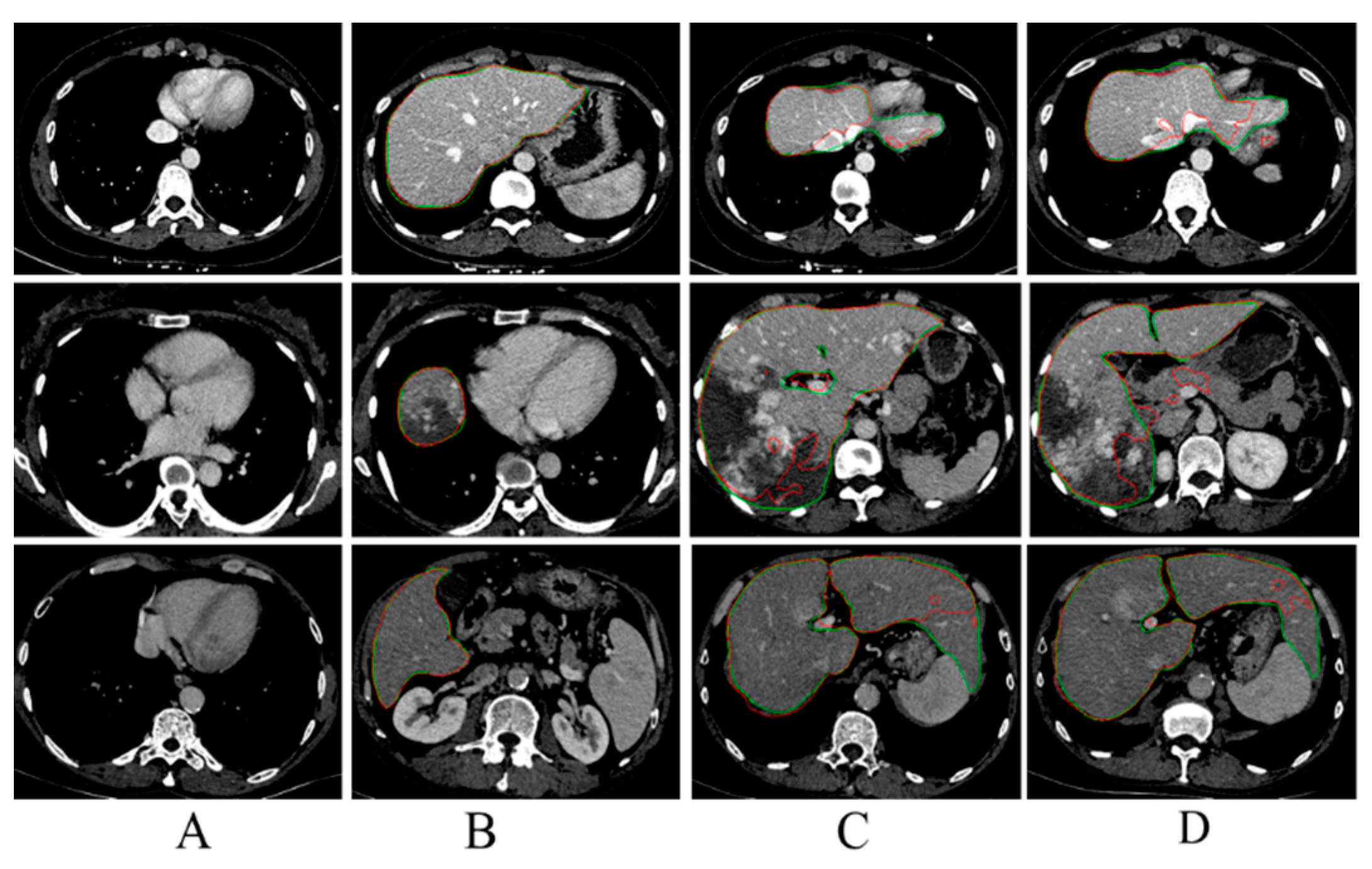
Automatic segmentation methods such as region growing, intensity thresholding, and deformable model-based methods have achieved automatic or semi-automatic segmentation to a certain extent, with good segmentation results. However, these models rely on hand-crafted features and have limited feature extraction ability. Recently, methods of deep learning, especially full convolutional networks (FCNs), have achieved great success on a broad array of recognition problems [2,3,4]. Many researchers advance this stream using deep learning methods in segmentation tasks such as liver [1,5,6,7], kidney [8], vessel [9,10,11] and pancreas [12,13,14]. All the models mentioned above are based on a large amount of data. However, there often are two kinds of data imbalance problems in the training process for the segmentation of CT scans: (i) data imbalance in images: the imbalance between background voxels and target voxels, as shown in Figure 1; (ii) data imbalance between images: the imbalance of hard or easy predicted examples in training datasets (the easily segmented slices are called easy samples or easy slices, while the difficult samples are defined as hard samples or hard slices) in training dataset. As shown in Figure 2A,B, the features of some slices are obvious and easy to segment. However, in some others, as shown in Figure 2C,D), the features of liver are not obvious, which may be due to poor quality of CT image or the liver self-defect (e.g., liver morphological variation, liver lesions, etc.), and it is difficult to accurately segment liver from these slices. Moreover, it is easy to qualitatively divide hard samples and easy samples according to the segmentation results, but it is difficult or almost impossible to describe the characteristics of hard samples and easy samples, and accurately distinguish them in training dataset before training process.
Using Dice coefficient [15] as the loss function in training process can solve the first kind of data imbalance by reducing or even ignoring the contribution of background voxels. However, due to the similarity between adjacent slices in medical images, and different training tasks (for example the same slice may be a hard example in liver segmentation task but an easy example in kidney or spleen segmentation task), it is difficult to classify medical images in training dataset automatically using traditional methods before the training process. When there are many easy samples, the contribution of hard slices will be overwhelmed in the training process, which could cause a significant reduction in the prediction ability of the model for difficult samples, and may even lead to overfitting. Therefore, it is necessary to classify the training samples and increase the proportion of hard samples in training datasets.
Recently, focal loss, which could automatically adjust the contribution of easy-negative samples in training process and rapidly focus on hard examples in every batch training process, has achieved great success in one-stage detector objection [16]. However, focal loss failed to change the imbalance between hard samples and easy samples in training dataset, the contribution of hard slices may still be overwhelmed in the training process. In order to solve or alleviate this imbalance problem, we introduce an online hard example enhancement method to increase the proportion of the hard samples in the training dataset. Frist, we use partial slices in the whole training dataset to train a pre-training model according to the needs of segmentation task, and then the pre-training model is used to distinguish hard samples and easy samples in the rest slices of the whole training dataset, i.e., adding the identified hard samples to the training datasets used in the pre-training processes. Second, the hard slices identified by pre-training model are selected and enhanced by flipping, and then these slices are added to the dataset used in pre-training process to enhance the ratio of hard slices in training dataset, and improve the contribution of hard slices in training process. Therefore, the basic purpose of pre-training strategy is to get a sample classifier, which could distinguish hard/easy slices according to actual task need.
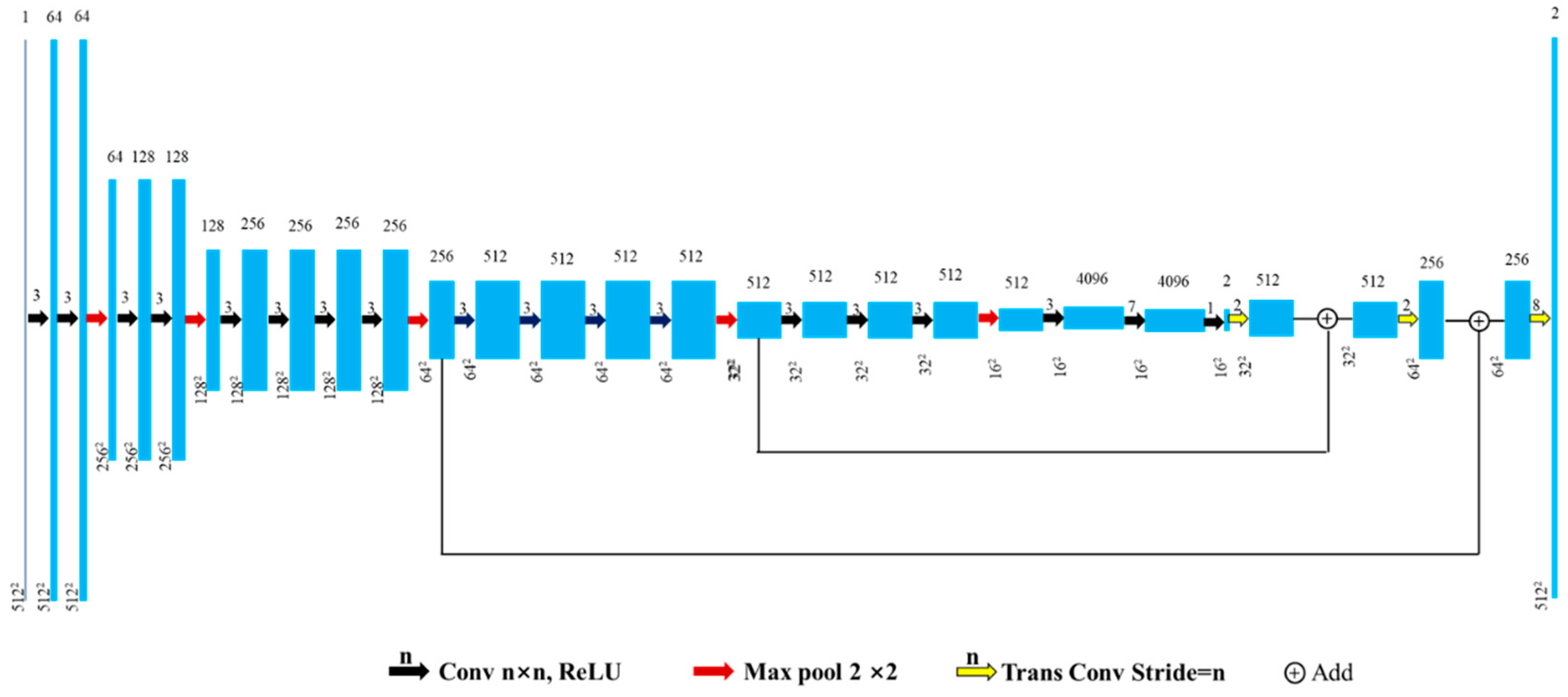
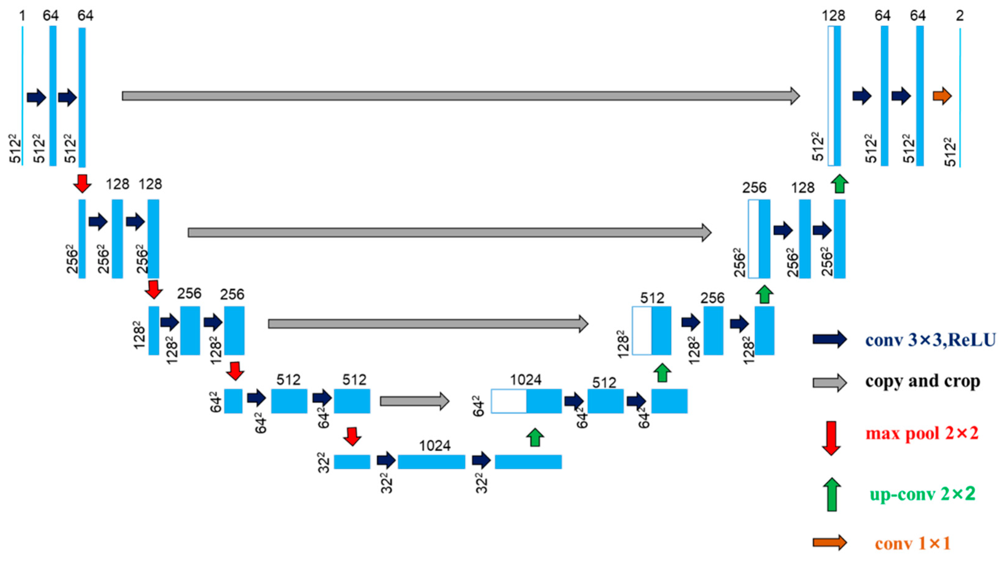
To demonstrate the effectiveness of the proposed method, we adopt a classical 2D FCN model based on VGG-16 [17] and 2D U-Net [3], as shown in Figure A1 and Figure A2 respectively, for the task of the liver segmentation, kidney segmentation and spleen segmentation from Computed Tomography (CT) scans.
2. Materials and Methods
2.1. Dataset and Processing
We test our method on datasets acquired from different scanners of different medical institutions. The collected dataset composes of 260 CT scans, with a largely varying in slice spacing from 0.45 mm to 5 mm. And 220 CT scans were randomly selected for training, the rest 40 cases for testing. For images pre-processing, the image intensity values were truncated to the range of [−150, 250] hounsfield unit (HU) to remove the irrelevant details [9].
2.2. Selection of Training Samples
Inspired by pre-training strategy, in this work, a pre-training model is used as a sample classifier to classify hard samples and easy samples in training dataset. Frist, the whole training dataset was divided into two parts (A and B) based on their simple statistics information (e.g., the number of slices in volume, the proportion of positive and negative samples in volume). In this way, the ratio of positive and negative slices in two subsets (A and B) can be guaranteed the same as that of the whole training dataset. Part A is used for the later sample classification and screening, while part B is used for model pre-training. Second, slices in part B are enhanced by flipping and mirroring, and then these enhanced slices are used in model pre-training process. And we get a pre-training model when model is trained to a set iteration (such as 5 × 10⁵ iterations in this work). Third, the pre-training model is used to predict slices in part A, and all slices in part A are simply divided into two categories, hard samples, and easy samples, by their Dice score. Next, the hard slices in part A are enhanced by flipping, and then added to the training dataset (part B) used in pre-training process. Finally, we continue the training process until reaching to the set 10 × 105 iterations, and then get the final segmentation model. Just 5 × 10⁵ iterations are needed in the final training process if 5 × 10⁵ iterations were done in the pre-training process and the pre-training model structure is consistent with the final model, while 10 × 105 iterations are needed in the final training stage if the pre-training model structure is inconsistent with the final model. In this study, we use the same model structure in pre-training process and final training stage.
2.3. Evaluation Metrics
Dice coefficient, which measures the amount of an agreement between two image regions, was used to evaluate the segmentation performance on the test dataset.
2.4. Implementation Details
Classical 2D FCN model structure and 2D U-Net are used for segmentation tasks from CT scans using the TensorFlow package [9]. We use stochastic gradient descent (SGD) with a mini-batch size 16. Inspired by [1], the “poly” learning rate policy where the current learning rate equals to the initial learning rate multiplying (1−(iterations)/(total_iterations))^power. We set the initial learning rate to 0.001 and the power to 0.9 and the models are trained for up to 10 × 105 iterations. We use the Dice coefficient as the loss function in the training process. For data augmentation, we adopt a random mirror, flip for all datasets. We use the aforementioned training strategy in the pre-training process and the final training stage.
3. Results
As for the strong similarity between adjacent slices in CT scans, we assume that the contribution of some slices could be replaced by others in the training process. To test this idea, we select partial cases at a certain ratio from the whole training dataset, based on their simple statistical information (e.g., the number of slices in volume, proportion of positive samples and negative samples in volume). And then the selected cases were enhanced by flipping and mirroring.
As shown in Table 1, reducing the number of training samples within a certain range has less influence on the segmentation ability of FCN. However, the prediction ability of FCN decreases significantly when the selection of training samples is further reduced. The max value, which refers to the best segmentation results of the model, has little change in different selection ratio (the ratio of training scans in part B to total number of scans in training dataset) experiments. Meanwhile, the min value, referring to the worst segmentation results of the model, decreases significantly when training samples decrease substantially. These phenomena are also observed in kidney segmentation and spleen segmentation from CT scans using FCN model, as shown in Table A1 and Table A2. Moreover, the same results were also discovered in liver segmentation, kidney segmentation and spleen segmentation tasks using U-Net model, as shown in Table A3, Table A4 and Table A5. These results suggest that there is redundancy in the training dataset, and that too little training data is harmful in the model training process.
As for the performance of FCN model begins to decline significantly when the selection ratio is less than 0.5, so we set selection ratio as 0.5 in the proposed model, and divide the training dataset into two parts (A and B) in liver segmentation. Slices in part B are used for model training, and we get the pre-training model after 5 × 10⁵ iterations. Using the pre-training model to predict slices in part A, we then simply classify these slices in part A into two categories, i.e., hard and easy simples, based on their Dice score. In the liver segmentation task using FCN model, we set the threshold to 0.923, the min Dice scores of baseline. Six thousand, two hundred and sixty-eight slices are classified as hard samples; however, 35,984 slices are classified as easy samples, almost 6-fold the number of hard samples. Hard samples in part A were enhanced by flipping and added to the dataset (part B) used in pre-training process. Then, we continue the training process until model reaching 10 × 105 iterations.
As shown in Table 1, the proposed model performs slightly better than the baseline in liver segmentation with a smaller training dataset. Moreover, adding hard examples has almost no effect on the max value of Dice score, but it can significantly increase the min value compared with the baseline. This indicates that increasing the ratio of hard samples in the training dataset has little influence on easily segmented cases, but could greatly improve the segmentation ability of model on hard samples.
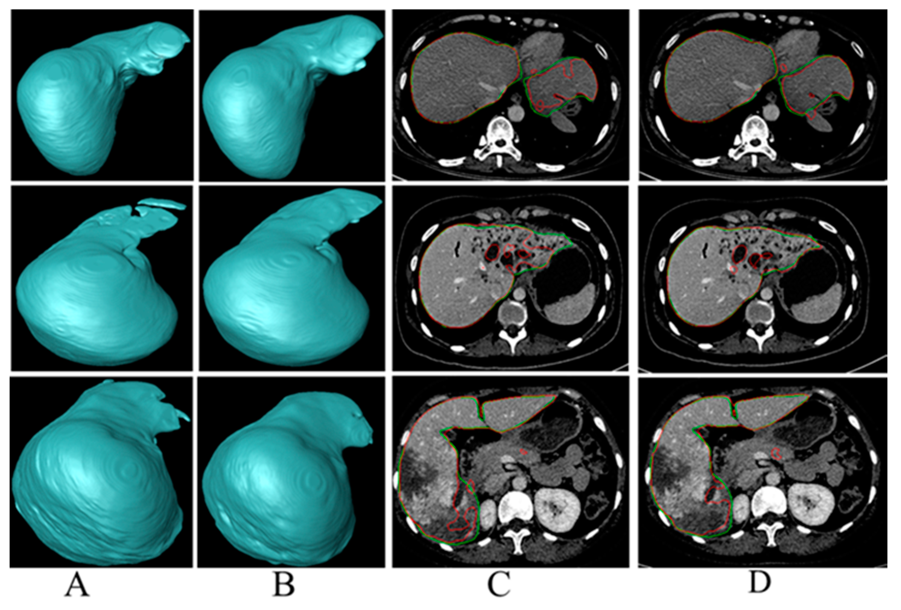
The segmentation results display in 3D form in Figure 3A,B show that the proposed method could enhance liver segmentation results, especially in some details. Liver segmentation results of hard examples have been greatly improved compared with the baseline, as shown in Figure 3C,D, which may be attributed to the increase of the number of hard samples in training dataset. The above results suggest that enhancing the proportion of hard samples in the training dataset could improve the prediction performance of FCN model in the liver segmentation task, as well as model’s ability to deal with hard samples.
4. Discussion
It is often thought that the more data, the better the performance in deep learning. However, in this work, we observed that a proper reduction of training samples in training process had little effect on the segmentation performance of model. This may be due to the strong similarity between two adjacent slices in CT images, which makes it difficult to ensure each image in the training dataset is independent from others; in other words, the contribution of some samples can be replaced by others in the training process. However, it is hard to screen out which one may be redundant. The relatively shallow network structure, which has relatively weak deep feature extraction capability, may be another reason for the phenomenon observed in this work. Meanwhile, the significantly reduced performance of the model in the case of a large reduction in training dataset also supports the point that the more data, the better the performance in deep learning.
Additionally, the same slices may play different roles in different segmentation tasks. For example, the positive-hard samples in the liver segmentation task may be negative-easy ones in kidney or spleen segmentation. Therefore, it is difficult to classify samples with the traditional unsupervised method. Inspired by the pre-training strategy, we use a pre-training method as a sample classifier to classify hard samples and easy samples in training dataset. We obtained better performance from the model after adding the enhanced hard examples.
Author Contributions
Conceptualization, Y.W. (Yi Wang) and B.F.; Data curation, Y.Z., Y.W. (Yizhu Wang), W.Y. and H.L. (Hancheng Lei); Funding acquisition, Y.W. (Yizhu Wang); Writing–original draft, Y.Z. and Y.W. (Yi Wang); Writing–review & editing, H.L. (Hongyu Long).
Funding
This work was supported by the National Natural Science Foundation of China (61876026, 61672120) and The Social Livelihood Science and Technology Innovation Special Project of CSTC (no. CSTC2015shmszx120002).
Conflicts of Interest
The authors declare no conflict of interest.
Appendix A
Figure A1.
FCN architecture. Each blue box corresponds to a multi-channel feature map. The number of channels is denoted on top of the box. The x-y-size is provided at the lower left edge of the box.
Figure A1.
FCN architecture. Each blue box corresponds to a multi-channel feature map. The number of channels is denoted on top of the box. The x-y-size is provided at the lower left edge of the box.

Figure A2.
U-net architecture. Each blue box corresponds to a multi-channel feature map. The number of channels is denoted on top of the box. The x-y-size is provided at the lower left edge of the box. White boxes represent copied feature maps. The arrows denote the different operations.
Figure A2.
U-net architecture. Each blue box corresponds to a multi-channel feature map. The number of channels is denoted on top of the box. The x-y-size is provided at the lower left edge of the box. White boxes represent copied feature maps. The arrows denote the different operations.


Table A1.
Kidney segmentation results on test dataset based on different selection ratio using FCN model.
Table A1.
Kidney segmentation results on test dataset based on different selection ratio using FCN model.
| Model | Dice Score | ||
|---|---|---|---|
| Mean | Min | Max | |
| selection ratio = 1, baseline | 0.9167 ± 0.13 | 0.8262 | 0.9698 |
| selection ratio = 0.8 | 0.9106 ± 0.089 | 0.8213 | 0.9703 |
| selection ratio = 0.5 | 0.9078 ± 0.114 | 0.822 | 0.9693 |
| selection ratio = 0.3 | 0.8835 ± 0.035 | 0.7935 | 0.9687 |
| selection ratio = 0.2 | 0.8511 ± 0.039 | 0.7724 | 0.9684 |
| proposed model | 0.9258 ± 0.067 | 0.8547 | 0.9693 |
Table A2.
Spleen segmentation results on test dataset based on different selection ratio using FCN model.
Table A2.
Spleen segmentation results on test dataset based on different selection ratio using FCN model.
| Model | Dice Score | ||
|---|---|---|---|
| Mean | Min | Max | |
| selection ratio = 1, baseline | 0.9773 ± 0.016 | 0.9364 | 0.9973 |
| selection ratio = 0.8 | 0.9762 ± 0.012 | 0.9379 | 0.9957 |
| selection ratio = 0.5 | 0.9767 ± 0.014 | 0.9359 | 0.9969 |
| selection ratio = 0.3 | 0.9714 ± 0.035 | 0.9358 | 0.997 |
| selection ratio = 0.2 | 0.8981 ± 0.139 | 0.7724 | 0.9965 |
| proposed model | 0.9801 ± 0.007 | 0.9563 | 0.9975 |
Table A3.
Liver segmentation results on test dataset based on different selection ratio using U-Net model.
Table A3.
Liver segmentation results on test dataset based on different selection ratio using U-Net model.
| Model | Dice Score | ||
|---|---|---|---|
| Mean | Min | Max | |
| selection ratio = 1, baseline | 0.9532 ± 0.035 | 0.9017 | 0.9875 |
| selection ratio = 0.8 | 0.9501 ± 0.031 | 0.908 | 0.9863 |
| selection ratio = 0.5 | 0.9486 ± 0.023 | 0.898 | 0.9867 |
| selection ratio = 0.3 | 0.9107 ± 0.057 | 0.834 | 0.9821 |
| selection ratio = 0.2 | 0.8932 ± 0.063 | 0.796 | 0.9806 |
| proposed model | 0.9604 ± 0.022 | 0.912 | 0.987 |
Table A4.
Kidney segmentation results on test dataset based on different selection ratio using U-Net model.
Table A4.
Kidney segmentation results on test dataset based on different selection ratio using U-Net model.
| Model | Dice Score | ||
|---|---|---|---|
| Mean | Min | Max | |
| selection ratio = 1, baseline | 0.9206 ± 0.073 | 0.8345 | 0.9732 |
| selection ratio = 0.8 | 0.9188 ± 0.092 | 0.8351 | 0.9725 |
| selection ratio = 0.5 | 0.9158 ± 0.113 | 0.8298 | 0.973 |
| selection ratio = 0.3 | 0.8735 ± 0.127 | 0.7653 | 0.9563 |
| selection ratio = 0.2 | 0.8621 ± 0.153 | 0.7549 | 0.9517 |
| proposed model | 0.9287 ± 0.028 | 0.8591 | 0.9708 |
Table A5.
Spleen segmentation results on test dataset based on different selection ratio using U-Net model.
Table A5.
Spleen segmentation results on test dataset based on different selection ratio using U-Net model.
| Model | Dice Score | ||
|---|---|---|---|
| Mean | Min | Max | |
| selection ratio = 1, baseline | 0.9795 ± 0.009 | 0.9473 | 0.9971 |
| selection ratio = 0.8 | 0.9803 ± 0.007 | 0.9482 | 0.9962 |
| selection ratio = 0.5 | 0.9780 ± 0.015 | 0.9367 | 0.9969 |
| selection ratio = 0.3 | 0.9704 ± 0.023 | 0.9289 | 0.9972 |
| selection ratio = 0.2 | 0.9057 ± 0.089 | 0.8124 | 0.9963 |
| proposed model | 0.9857 ± 0.005 | 0.9579 | 0.9969 |
References
- Li, X.; Chen, H.; Qi, X.; Dou, Q.; Fu, C.W.; Heng, P.A. H-Dense UNet: hybrid densely connected UNet for liver and tumor segmentation from CT volumes. IEEE Trans. Med. Imaging 2018, 37, 2663–2674. [Google Scholar] [CrossRef] [PubMed]
- Shaoqing, R.; Kaiming, H.; Girshick, R.; Xiangyu, Z.; Jian, S. Object detection networks on convolutional feature maps. IEEE Trans. Pattern Anal. Mach. Intell. 2017, 39, 1476–1481. [Google Scholar]
- Ronneberger, O.; Fischer, P.; Brox, T. U-net: Convolutional networks for biomedical image segmentation. In Proceedings of the International Conference on Medical Image Computing and Computer-Assisted Intervention, Munich, Germany, 5–9 October 2015; pp. 234–241. [Google Scholar]
- Hwang, H.; Rehman, H.Z.U.; Lee, S. 3D U-Net for skull stripping in brain MRI. Appl. Sci. 2019, 9, 569. [Google Scholar] [CrossRef]
- Vorontsov, E.; Tang, A.; Pal, C.; Kadoury, S. Liver lesion segmentation informed by joint liver segmentation. In Proceedings of the 2018 IEEE 15th International Symposium on Biomedical Imaging (ISBI), Washington, DC, USA, 4–7 April 2018; pp. 1332–1335. [Google Scholar]
- Lu, F.; Wu, F.; Hu, P.J.; Peng, Z.Y.; Kong, D.X. Automatic 3D liver location and segmentation via convolutional neural network and graph cut. Int J. CARS 2017, 12, 171–182. [Google Scholar] [CrossRef] [PubMed]
- Kaluva, K.C.; Khened, M.; Kori, A.; Krishnamurthi, G. 2D-Densely Connected Convolution Neural Networks for automatic Liver and Tumor Segmentation. arXiv 2018, arXiv:1802.02182. [Google Scholar]
- Zhao, F.; Gao, P.; Hu, H.; He, X.; Hou, Y.; He, X. Efficient kidney segmentation in micro-CT based on multi-atlas registration and random forests. IEEE Access 2018, 6, 43712–43723. [Google Scholar] [CrossRef]
- Moccia, S.; Momi, E.; Hadji, S.E.; Mattos, L.S. Efficient kidney segmentation in micro-CT based on multi-atlas registration and random forests. Comput. Meth. Prog Bio. 2018, 158, 71–91. [Google Scholar] [CrossRef] [PubMed]
- Jin, Q.G.; Meng, Z.P.; Tuan, D.P.; Chen, Q.; Wei, L.Y.; Su, R. DUNet: A deformable network for retinal vessel segmentation. arXiv 2018, arXiv:1811.01206. [Google Scholar]
- Tetteh, G.; Efremov, V.; Forkert, N.D.; Schneider, M.; Kirschke, J.; Weber, B.; Zimmer, C.; Piraud, M.; Menze, B.H. DeepVesselNet: vessel segmentation, centerline prediction, and bifurcation detection in 3-D angiographic volumes. arXiv 2018, arXiv:1803.09340. [Google Scholar]
- Cai, J.L.; Lu, L.; Xing, F.Y.; Yang, L. Pancreas segmentation in CT and MRI images via domain specific network designing and recurrent neural contextual learning. arXiv 2018, arXiv:1803.11303. [Google Scholar]
- Roth, H.R.; Lu, L.; Lay, N.; Harrison, A.P.; Farag, A.; Sohn, A.; Summers, R.M. Spatial aggregation of holistically-nested convolutional neural networks for automated pancreas localization and segmentation. Med. Image Anal. 2018, 45, 94–107. [Google Scholar] [CrossRef] [PubMed]
- Yu, Q.H.; Xie, L.X.; Wang, Y.; Zhou, Y.Y.; Fishman, E.K.; Yuille, A.L. Recurrent Saliency Transformation Network: Incorporating Multi-Stage Visual Cues for Small Organ Segmentation. In Proceedings of the 2018 IEEE Conference on Computer Vision and Pattern Recognition (CVPR), Salt Lake City, UT, USA, 18–22 June 2018; pp. 8280–8289. [Google Scholar]
- Taha, A.A.; Hanbury, A. Metrics for evaluating 3D medical image segmentation: Analysis, selection, and tool. BMC Med. Imaging 2015, 15, 29. [Google Scholar] [CrossRef] [PubMed]
- Lin, T.Y.; Goyal, P.; Girshick, R.; He, K.; Dollar, P. Focal loss for dense object detection. In Proceedings of the IEEE International Conference on Computer Vision (ICCV), Venice, Italy, 22–29 October 2017; pp. 2980–2988. [Google Scholar]
- Long, J.; Shelhamer, E.; Darrell, T. Fully Convolutional Networks for Semantic Segmentation. In Proceedings of the IEEE Conference on Computer Vision and Pattern Recognition (CVPR), Boston, MA, USA, 7–12 June 2015; pp. 3431–3440. [Google Scholar]
Figure 1.
Examples of the imbalance between background voxels and target voxels in images. Each row shows a CT scan from individual patients. The read regions denote the liver.
Figure 1.
Examples of the imbalance between background voxels and target voxels in images. Each row shows a CT scan from individual patients. The read regions denote the liver.
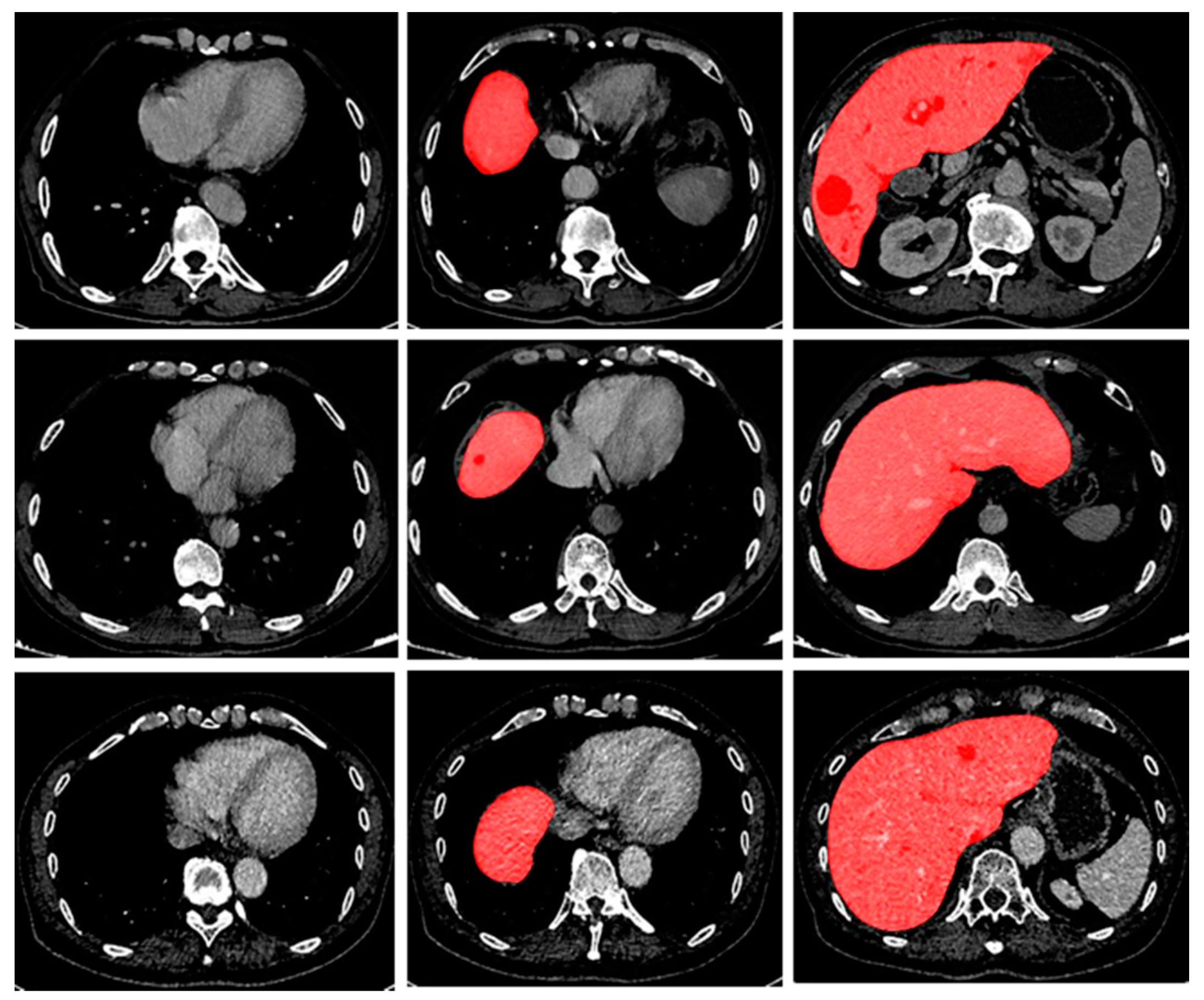
Figure 2.
Examples of easy and hard predicted slices in CT scans. The predicted results are based on the FCN model with 10 × 105 iterations. (A,B) display the easy samples; (C,D) display the hard slices. Blue and red lines denote ground truth and prediction results. Each row shows results acquired from an individual case.

Figure 3.
Results of Liver segmentation using FCN model. (A,B) display the 3D liver segmentation result of the baseline and proposed a model, respectively; (C,D) display the hard samples liver segmentation results of the baseline and proposed a model, respectively; Blue and red lines in C and D denote ground truth and prediction results. Each row shows results acquired from an individual case.

Table 1.
Liver segmentation results on test dataset based on different selection ratio using FCN model.
Table 1.
Liver segmentation results on test dataset based on different selection ratio using FCN model.
| Model | Dice Score | ||
|---|---|---|---|
| Mean | Min | Max | |
| selection ratio = 1, baseline | 0.9705 ± 0.011 | 0.923 | 0.9856 |
| selection ratio = 0.8 | 0.9706 ± 0.011 | 0.921 | 0.9853 |
| selection ratio = 0.5 | 0.9702 ± 0.013 | 0.9124 | 0.9843 |
| selection ratio = 0.3 | 0.9512 ± 0.035 | 0.8635 | 0.9844 |
| selection ratio = 0.2 | 0.9475 ± 0.039 | 0.812 | 0.9817 |
| proposed model | 0.9789 ± 0.012 | 0.947 | 0.9854 |
© 2019 by the authors. Licensee MDPI, Basel, Switzerland. This article is an open access article distributed under the terms and conditions of the Creative Commons Attribution (CC BY) license (http://creativecommons.org/licenses/by/4.0/).
Share and Cite
MDPI and ACS Style
Zhang, Y.; Wang, Y.; Wang, Y.; Fang, B.; Yu, W.; Long, H.; Lei, H. Data Balancing Based on Pre-Training Strategy for Liver Segmentation from CT Scans. Appl. Sci. 2019, 9, 1825. https://doi.org/10.3390/app9091825
AMA Style
Zhang Y, Wang Y, Wang Y, Fang B, Yu W, Long H, Lei H. Data Balancing Based on Pre-Training Strategy for Liver Segmentation from CT Scans. Applied Sciences. 2019; 9(9):1825. https://doi.org/10.3390/app9091825
Chicago/Turabian StyleZhang, Yong, Yi Wang, Yizhu Wang, Bin Fang, Wei Yu, Hongyu Long, and Hancheng Lei. 2019. "Data Balancing Based on Pre-Training Strategy for Liver Segmentation from CT Scans" Applied Sciences 9, no. 9: 1825. https://doi.org/10.3390/app9091825
Note that from the first issue of 2016, this journal uses article numbers instead of page numbers. See further details here.