Robust Adaptive Path Following Control of an Unmanned Surface Vessel Subject to Input Saturation and Uncertainties


Abstract
:1. Introduction
- (1)
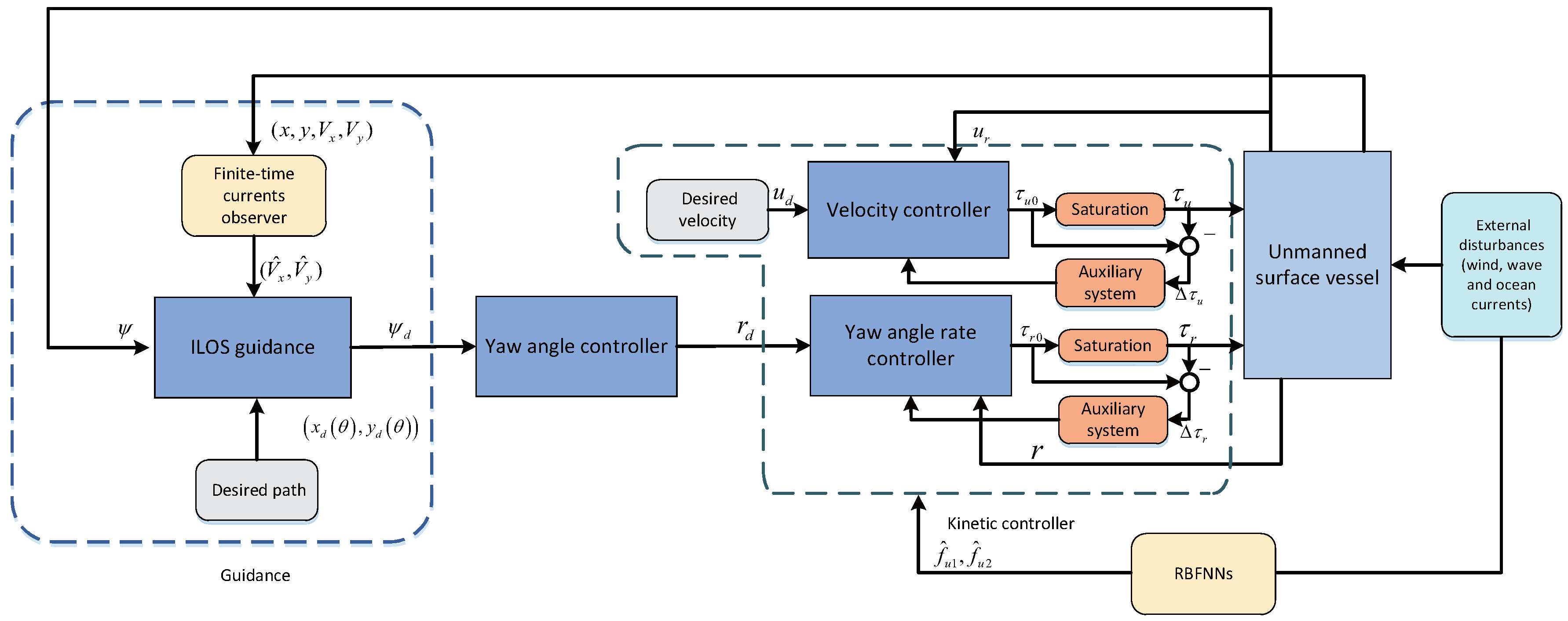
- A finite-time currents observer based LOS guidance is presented to obtain the desired yaw angle and estimate the unknown time-varying ocean currents precisely, which significantly influences the performance of the control subsystem.
- (2)
- The RBF neural networks are incorporated into the kinetic controller to solve the uncertainties, which does not require any prior knowledge of the dynamics of the USV and disturbances, and the adaptive laws are designed to estimate the compound bounds of approximating errors and external time-varying disturbances.
- (3)
- The input constraint effect is analyzed with auxiliary systems and the states of auxiliary systems are utilized to make compensations for input saturation, which attenuates the challenge of the actuators.
2. Preliminaries and Problem Formulation
2.1. RBFNN Approximation
2.2. USV Model
2.3. Control Objective
3. Main Results
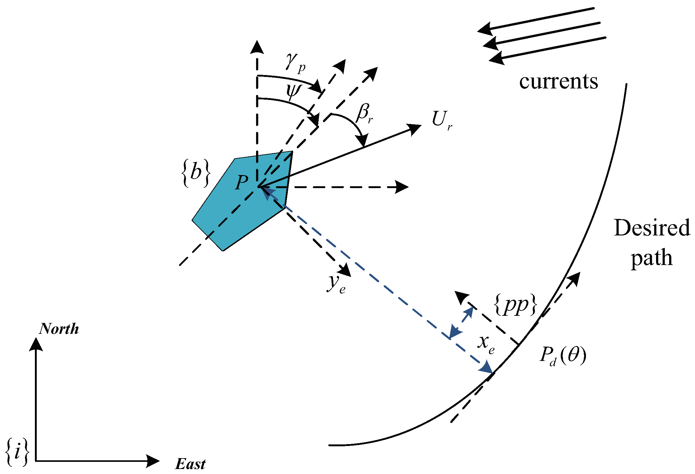
3.1. Guidance
3.1.1. Estimations of Ocean Currents
3.1.2. Design of Kinematic Controller
3.2. Design of Kinetic Controller
3.3. Stability Analysis
3.4. Sway Dynamics
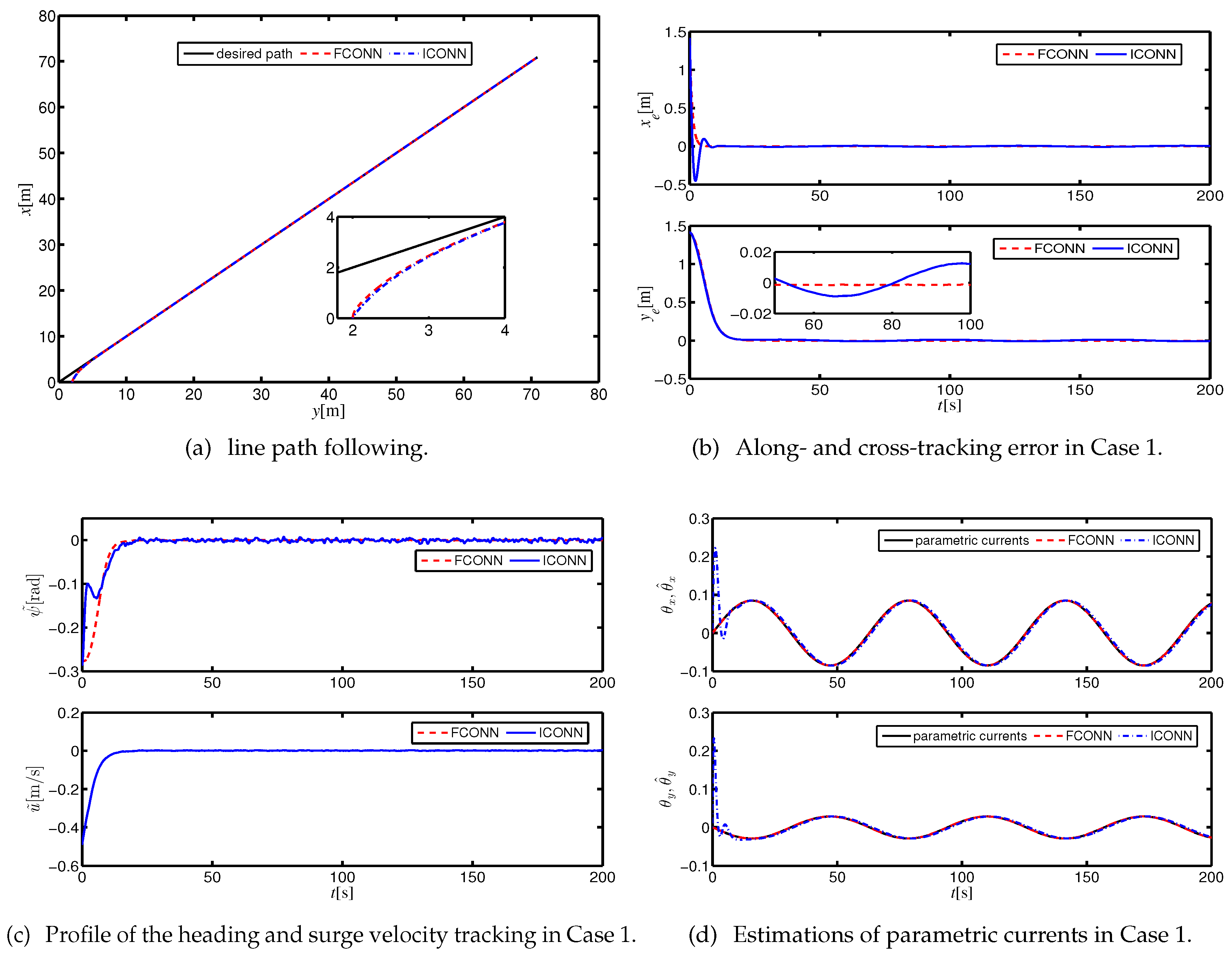
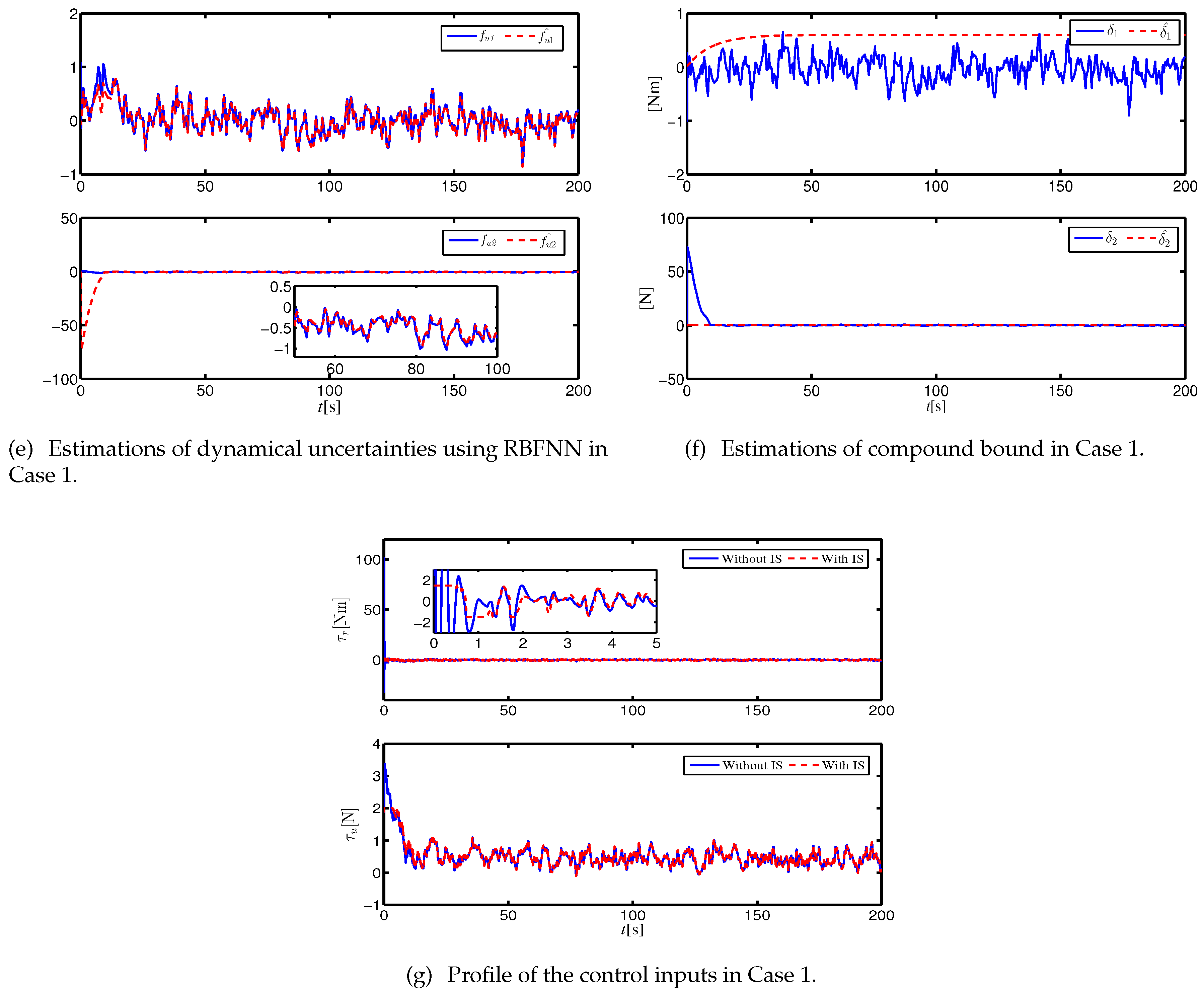
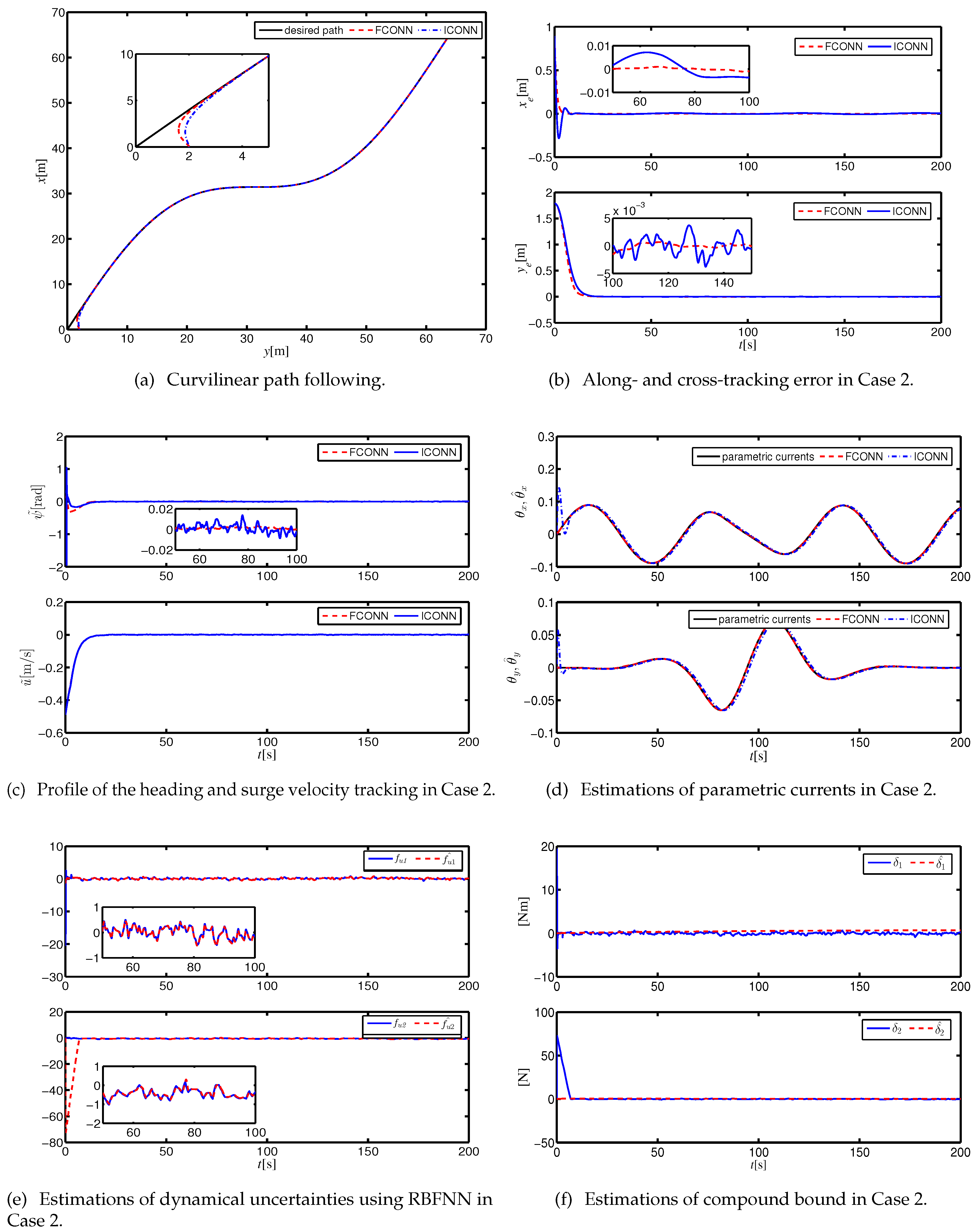
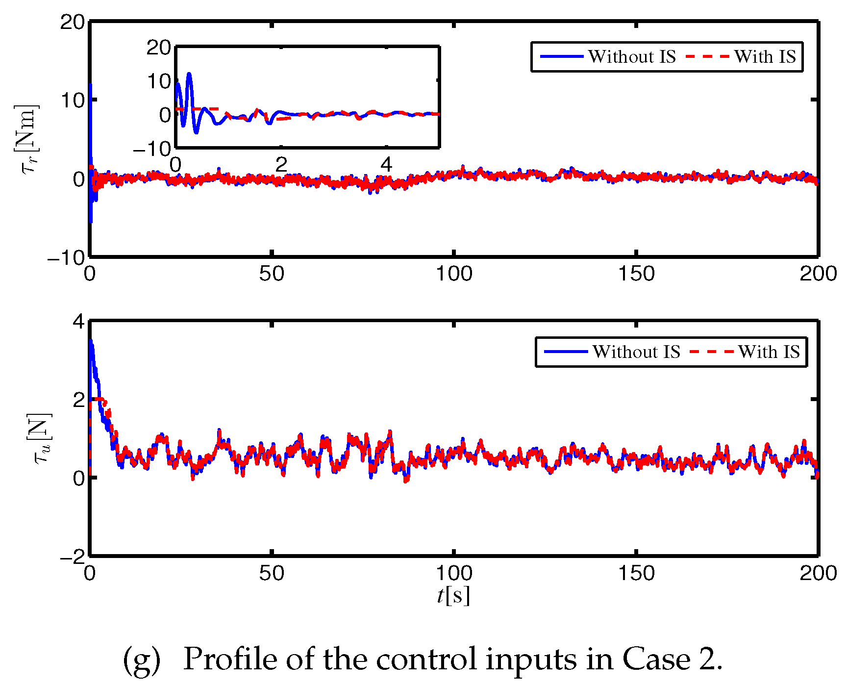
4. Simulations
5. Conclusions
Author Contributions
Funding
Conflicts of Interest
References
- Liu, Z.; Zhang, Y.; Yu, X.; Yuan, C. Unmanned surface vehicles: An overview of developments and challenges. Annu. Rev. Control. 2016, 41, 71–93. [Google Scholar] [CrossRef]
- Ashrafiuon, H.; Muske, K.R.; Mcninch, L.C. Review of nonlinear tracking and setpoint control approaches for autonomous underactuated marine vehicles. In Proceedings of the 2010 American Control Conference, Baltimore, MD, USA, 30 June–2 July 2010; pp. 5203–5211. [Google Scholar]
- Do, K.D.; Pan, J. Control of ships and underwater vehicles. In Advances in Industrial Control; Springer: London, UK, 2009; pp. 40–42. ISBN 978-1-84882-729-5. [Google Scholar]
- Caccia, M.; Bibuli, M.; Bono, R.; Bruzzone, G. Basic navigation, guidance and control of an unmanned surface vehicle. Auton. Robot. 2008, 25, 349–365. [Google Scholar] [CrossRef]
- Breivik, M.; Fossen, T.I. Path following for marine surface vessels. In Proceedings of the Oceans ’04 MTS/IEEE Techno-Ocean ’04, Kobe, Japan, 9–12 November 2004; pp. 2282–2289. [Google Scholar]
- Fossen, T.I.; Breivik, M.; Skjetne, R. Line-of-sight path following of underactuated marine craft. In Proceedings of the IFAC Manoeuvring and control of Marine Craft, Girona, Spain, 17–19 September 2003; pp. 211–216. [Google Scholar]
- Fossen, T.I.; Pettersen, K.Y. On uniform semiglobal exponential stability (usges) of proportional line-of-sight guidance laws. Automatica 2014, 50, 2912–2917. [Google Scholar] [CrossRef]
- Borhaug, E.; Pavlov, A.; Pettersen, K.Y. Integral LOS control for path following of underactuated marine surface vessels in the presence of constant ocean currents. In Proceedings of the 47th IEEE conference on Decision and Control, Cancun, Mexico, 9–11 September 2008; pp. 4984–4991. [Google Scholar]
- Lekkas, A.M.; Fossen, T.I. Integral los path following for curved paths based on a monotone cubic hermite spline parametrization. IEEE Trans. Control. Syst. Technol. 2014, 22, 2287–2301. [Google Scholar] [CrossRef]
- Fossen, T.I.; Lekkas, A.M. Direct and indirect adaptive integral line-of-sight path-following controllers for marine craft exposed to ocean currents. Int. J. Adapt. Control. Signal Process. 2017, 31, 445–463. [Google Scholar] [CrossRef]
- Fossen, T.I.; Pettersen, K.Y.; Galeazzi, R. Line-of-sight path following for dubins paths with adaptive sideslip compensation of drift forces. IEEE Trans. Control. Syst. Technol. 2015, 23, 820–827. [Google Scholar] [CrossRef]
- Liu, L.; Wang, D.; Peng, Z. Eso-based line-of-sight guidance law for path following of underactuated marine surface vehicles with exact sideslip compensation. IEEE J. Ocean. Eng. 2017, 42, 477–487. [Google Scholar] [CrossRef]
- Wang, N.; Sun, Z.; Yin, J.; Su, S.F.; Sharma, S. Finite-time observer based guidance and control of underactuated surface vehicles with unknown sideslip angles and disturbances. IEEE Access 2018, 6, 14059–14070. [Google Scholar] [CrossRef]
- Wang, W.; Huang, J.; Wen, C.; Fan, H. Distributed adaptive control for consensus tracking with application to formation control of nonholonomic mobile robots. Automatica 2014, 50, 1254–1263. [Google Scholar] [CrossRef]
- Miao, J.; Wang, S.; Tomovic, M.M.; Zhao, Z. Compound line-of-sight nonlinear path following control of underactuated marine vehicles exposed to wind, waves, and ocean currents. Nonlinear Dyn. 2017, 89, 1–19. [Google Scholar] [CrossRef]
- Do, K.D. Global robust adaptive path-tracking control of underactuated ships under stochastic disturbances. Ocean. Eng. 2016, 111, 267–278. [Google Scholar] [CrossRef]
- Liu, S.; Liu, Y.; Wang, N. Nonlinear disturbance observer-based backstepping finite-time sliding mode tracking control of underwater vehicles with system uncertainties and external disturbances. Nonlinear Dyn. 2017, 88, 1–12. [Google Scholar] [CrossRef]
- Du, J.; Hu, X.; Krstić, M.; Sun, Y. Robust dynamic positioning of ships with disturbances under input saturation. Automatica 2016, 73, 207–214. [Google Scholar] [CrossRef]
- Sun, Z.; Zhang, G.; Yi, B.; Zhang, W. Practical proportional integral sliding mode control for underactuated surface ships in the fields of marine practice. Ocean. Eng. 2017, 142, 217–223. [Google Scholar] [CrossRef]
- Roy, S.; Roy, S.B.; Kar, I.N. Adaptive-robust control of euler-lagrange systems with linearly parametrizable uncertainty bound. IEEE Trans. Control. Syst. Technol. 2017, 26, 1842–1850. [Google Scholar] [CrossRef]
- Roy, S.; Roy, S.B.; Kar, I.N. A New Design Methodology of Adaptive Sliding Mode Control for a Class of Nonlinear Systems with State Dependent Uncertainty Bound. In Proceedings of the 15th International Workshop on Variable Structure Systems, Graz, Austria, 9–11 September 2018; pp. 414–419. [Google Scholar]
- Wang, N.; Er, M.J.; Sun, J.C.; Liu, Y.C. Adaptive robust online constructive fuzzy control of a complex surface vehicle system. IEEE Trans. Cybern. 2017, 46, 1511–1523. [Google Scholar] [CrossRef]
- Zheng, Z.; Sun, L. Path following control for marine surface vessel with uncertainties and input saturation. Neurocomputing 2016, 177, 158–167. [Google Scholar] [CrossRef]
- Liu, L.; Wang, D.; Peng, Z. Path following of marine surface vehicles with dynamical uncertainty and time-varying ocean disturbances. Neurocomputing 2016, 173, 799–808. [Google Scholar] [CrossRef]
- Zheng, Z.; Feroskhan, M. Path following of a surface vessel with prescribed performance in the presence of input saturation and external disturbances. IEEE/ASME Trans. Mechatronics 2017, 22, 2564–2575. [Google Scholar] [CrossRef]
- Roy, S.; Shome, S.N.; Nandy, S.; Ray, R.; Kumar, V. Trajectory following control of auv: A robust approach. J. Inst. Eng. India Series C 2013, 94, 253–265. [Google Scholar] [CrossRef]
- Shtessel, Y.B.; Shkolnikov, I.A.; Levant, A. Smooth second-order sliding modes: Missile guidance application. Automatica 2007, 43, 1470–1476. [Google Scholar] [CrossRef]
- Chen, M.; Ge, S.S.; Ren, B. Adaptive tracking control of uncertain mimo nonlinear systems with input constraints. Automatica 2011, 47, 452–465. [Google Scholar] [CrossRef]
- Polycarpou, M.M.; Ioannou, P.A. A robust adaptive nonlinear control design. Automatica 1996, 32, 423–427. [Google Scholar] [CrossRef]
- Krstic, M.; Kanellakopoulos, I.; Kokotovic, P.V. Nonlinear and adaptive control. In Lecture Notes in Control and Information; Sciences: New York, NY, USA, 1995; pp. 511–514. ISBN 9780471127321. [Google Scholar]
- Fredriksen, E.; Pettersen, K.Y. Global k-exponential way-point maneuvering of ships: Theory and experiments. Automatica 2009, 42, 677–687. [Google Scholar] [CrossRef]
- Fossen, T.I. How to incorporate wind, waves and ocean currents in the marine craft equations of motion. In Proceedings of the 9th IFAC Conference on Manoeuvring and Control of Marine Craft, Arenzano, Italy, 19–21 September 2012; pp. 126–131. [Google Scholar]


| Notation | Value | Natation | Value | Natation | Value | Natation | Value | Natation | Value |
|---|---|---|---|---|---|---|---|---|---|
| 1 | 4 | 500 | 20 | 0.01 | |||||
| 2 | 0.01 | 50 | 0.01 | 1 | |||||
| 4 | 0.03 | 0.05 | 0.01 | 2.51 | |||||
| 5 | 1.2 | 0.05 | 0.1 | ||||||
| 100 | 1.2 | 50 | 0.1 |
| Control Law | Line Path Following | Curvilinear Path Following | ||
|---|---|---|---|---|
| IAE() | ITAE() | IAE() | ITAE() | |
| FCONN | 1.92 | 5.78 | 2.58 | 9.01 |
| IAONN | 4.18 | 13.12 | 7.32 | 20.32 |
© 2019 by the authors. Licensee MDPI, Basel, Switzerland. This article is an open access article distributed under the terms and conditions of the Creative Commons Attribution (CC BY) license (http://creativecommons.org/licenses/by/4.0/).
Share and Cite
Fan, Y.; Huang, H.; Tan, Y. Robust Adaptive Path Following Control of an Unmanned Surface Vessel Subject to Input Saturation and Uncertainties. Appl. Sci. 2019, 9, 1815. https://doi.org/10.3390/app9091815
Fan Y, Huang H, Tan Y. Robust Adaptive Path Following Control of an Unmanned Surface Vessel Subject to Input Saturation and Uncertainties. Applied Sciences. 2019; 9(9):1815. https://doi.org/10.3390/app9091815
Chicago/Turabian StyleFan, Yunsheng, Hongyun Huang, and Yuanyuan Tan. 2019. "Robust Adaptive Path Following Control of an Unmanned Surface Vessel Subject to Input Saturation and Uncertainties" Applied Sciences 9, no. 9: 1815. https://doi.org/10.3390/app9091815
APA StyleFan, Y., Huang, H., & Tan, Y. (2019). Robust Adaptive Path Following Control of an Unmanned Surface Vessel Subject to Input Saturation and Uncertainties. Applied Sciences, 9(9), 1815. https://doi.org/10.3390/app9091815