The Method of Fundamental Solutions for Three-Dimensional Nonlinear Free Surface Flows Using the Iterative Scheme

Abstract

In this article, we present a meshless method based on the method of fundamental solutions (MFS) capable of solving free surface flow in three dimensions. Since the basis function of the MFS satisfies the governing equation, the advantage of the MFS is that only the problem boundary needs to be placed in the collocation points. For solving the three-dimensional free surface with nonlinear boundary conditions, the relaxation method in conjunction with the MFS is used, in which the three-dimensional free surface is iterated as a movable boundary until the nonlinear boundary conditions are satisfied. The proposed method is verified and application examples are conducted. Comparing results with those from other methods shows that the method is robust and provides high accuracy and reliability. The effectiveness and ease of use for solving nonlinear free surface flows in three dimensions are also revealed.

1. Introduction

Accurate determination of the unknown phreatic line is regarded as one of the most important considerations for affecting the safety of an embankment dam or weirs, since failure of the earth–filled structure occurs because of piping and internal erosion mainly from seepage [1]. The determination of the phreatic line in seepage flow is a nonlinear problem which needs to find the location of the movable surface from the nonlinear boundary conditions [2]. The free surface problems can be solved using mesh–based methods with an adaptive mesh [3,4,5,6] or a fixed mesh [7,8,9,10,11,12]. Among the methods, the extended pressure method [13] based on finite differences is probably the simplest one for free surface calculation. Computational techniques for calculating two–dimensional free surface flows are well-established [14,15,16,17,18,19,20,21]. However, solving three-dimensional free surface flow problems needs to deal with three-dimensional geometric complexity. Mesh-based methods for handling the complexity of three-dimensional boundary conditions require sophisticated remeshing scheme. To have a successful three-dimensional mesh generation algorithm is, therefore, quite a challenging task.

Comparing to conventional mesh-based methods, meshless methods are relatively simple because only arbitrary collocation points need to be placed on the physical domain [22]. In particular, the collocation points may be placed only on the boundary for the method of fundamental solutions (MFS) [23,24,25,26,27,28,29] because the basis function is the fundamental solution which satisfies the governing equation. The basic idea of the MFS is to represent the unknown as the linear combination of basis functions which are the fundamental solutions using the addition theorem [28]. The solutions are computed by fundamental solutions using many sources which must be collocated outside the domain of the problem. Since the boundary conditions are applied at boundary points, the intensities of source points (or the coefficients) can be obtained by solving the system of simultaneous linear equations. To avoid the treatment of singularities, the source points of the MFS must be collocated out of the domain [30]. As a result, the MFS does not need to deal with the singularities, meshes, and numerical integrations. With the advantage of the boundary-type meshless method, only the collocation points on the moving surface have to be renewed during iteration for the computation of the position of the three-dimensional nonlinear free surface [1]. It avoids the most difficult task for handling the three-dimensional geometric complexity. As the problem of the free surface flow is nonlinear, it is necessary to introduce the iterative strategies to solve the nonlinear problem. Two common fundamental schemes are used. They are the fixed-point iteration [31,32] and the Newton type schemes [33]. The relaxation scheme [34,35,36] based on the fixed-point iteration scheme with a relaxation factor is adopted in this study for solving the nonlinear free surface problems in the three-dimensional domain. For solving the nonlinear problem, the iterations are required to match the boundary conditions on the moving surface.

To the best of the authors’ knowledge, the pioneering work which uses the proposed MFS to solve the nonlinear free surface flows in three dimensions has not been reported in previous studies yet. We therefore propose a moving meshless method based on the MFS capable of solving three-dimensional free surface flow problems over arbitrary geometries in this article. Since the basis function of the MFS is the solution derived from the governing equation, the MFS is categorized into the meshless method in which only the domain boundary needs to be discretized by placing the collocation points. For solving the three-dimensional free surface with nonlinear boundary conditions, the relaxation method in conjunction with the MFS is used, in which the three-dimensional free surface is iterated as the movable surface until the nonlinear boundary conditions are satisfied. The proposed method is verified and application examples are performed.

The remainder of this paper is as follows. We introduce the governing equation of the three-dimensional free surface flow in Section 2. Section 3 is devoted to give the formulation of the MFS and the iterative scheme for finding the free surface are also presented. In Section 4, validation examples of the proposed method are conducted. In Section 5, application examples are also carried out to evaluate the performance of the proposed MFS. In Section 6, a specific discussion of this paper is given. Finally, conclusions are presented in Section 7.

2. The Governing Equation

The governing equation in three dimensions for the seepage flow through a homogenous porous media is as follows:

$$\Delta h(x,y,z)=0\mathrm{in}\Omega ,$$

(1)

with

$$h(x,y,z)=g\mathrm{on}{\Gamma }_D,$$

(2)

$$\frac{\partial h(x,y,z)}{\partial n}=f\mathrm{on}{\Gamma }_N,$$

(3)

where $h$ is the total head, $\Delta$ is the Laplacian, $\Omega$ represents the boundary of the problem, $n$ denotes the normal vector, $\Gamma \in {\Gamma }_D\cup {\Gamma }_N$ is the boundary of $\Omega$, $g$ and $f$ denote the Dirichlet and Neumann boundary values, ${\Gamma }_D$ denotes the Dirichlet boundary, and ${\Gamma }_N$ denotes the Neumann boundary. As demonstrated in Figure 1, the boundary conditions of the free surface flow in three dimensions through a rectangular dam can be presented by ${\Gamma }_{abcd}$, ${\Gamma }_{bcef}$, ${\Gamma }_{fegh}$, ${\Gamma }_{hgij}$, ${\Gamma }_{adij}$, ${\Gamma }_{abhj}$ and ${\Gamma }_{dcgi}$. The Dirichlet boundary conditions are imposed on the ${\Gamma }_{bcef}$ and ${\Gamma }_{adij}$, respectively.

$$h={\mathrm{H}}_2\mathrm{on}{\Gamma }_{adij},$$

(4)

$$h={\mathrm{H}}_1\mathrm{on}{\Gamma }_{bcef}.$$

(5)

According to the Bernoulli equation, the total head can be expressed as

$$h=z+\frac{p}{\gamma },$$

(6)

where $z$ is the head above the sea level, $p$ is the pore water pressure, and $\gamma$ is the water unit weight. On the free surface boundary, ${\Gamma }_{hgij}$, the boundary conditions are given as follows:

$$\frac{\partial h}{\partial n}=0,h=z\mathrm{on}{\Gamma }_{hgij}.$$

(7)

On the seepage face boundary, ${\Gamma }_{fegh}$, the boundary condition is depicted as

$$h=z\mathrm{on}{\Gamma }_{fegh}.$$

(8)

On boundaries, ${\Gamma }_{abcd}$, ${\Gamma }_{abhj}$ and ${\Gamma }_{dcgi}$, the Neumann boundary conditions may be given as follows:

$$\frac{\partial h}{\partial n}=0\mathrm{on}{\Gamma }_{abcd},{\Gamma }_{abhj}\mathrm{and}{\Gamma }_{dcgi}.$$

(9)

Since $h=z$ is unknown and needs to be computed iteratively, we adopt the MFS to solve the governing equation for the nonlinear free surface seepage flow.

3. The Method of Fundamental Solutions

To obtain the three-dimensional free surface with nonlinear boundary conditions, the relaxation method in conjunction with the MFS was used. The formulation of the MFS and the relaxation method for finding the free surface are described in the following section.

3.1. The Fundamental Solution of the Laplace Equation

A fundamental solution for a linear partial differential equation with regard to the Dirac delta function is the solution of the inhomogeneous equation.

$$\Delta G(\mathbf{x},\mathbf{y})=\delta (\mathbf{x}-\mathbf{y}),$$

(10)

where $G(\mathbf{x},\mathbf{y})$ is the three-dimensional fundamental solution for the Laplace equation, $\mathbf{x}$ is the spatial coordinate which is collocated on the boundary, $\mathbf{y}$ is the coordinate of source points, and $\delta (\mathbf{x}-\mathbf{y})$ is the Dirac delta function. In the MFS, the unknown is assumed to be the linear combination of fundamental solutions of the governing equation using source points. The solution of the Laplace equation in three dimensions is approximated as follows:

$$h(\mathbf{x})\approx {\displaystyle \sum _{j=1}^N{\alpha }_{j}G(\mathbf{x},{\mathbf{y}}_j)},\mathbf{x}\in \Omega ,$$

(11)

where ${\alpha }_j$ is the coefficient or the intensity of source points, ${\mathbf{y}}_j$ is the source placed outside the domain, and $N$ is the source number. The fundamental solution of three-dimensional Laplace equation is then expressed as

$$G(\mathbf{x},{\mathbf{y}}_j)=\frac{1}{4\pi r_j},$$

(12)

where $r_j=\left|\mathbf{x}-{\mathbf{y}}_j\right|$ is the distance between the $\mathbf{x}$ and j-th sources ${\mathbf{y}}_j$. Applying the boundary conditions, the following equations can be obtained:

$$h({\mathbf{x}}_k)\approx {\displaystyle \sum _{j=1}^N{\alpha }_{j}G({\mathbf{x}}_k,{\mathbf{y}}_j)}=g({\mathbf{x}}_k),$$

(13)

$$\frac{\partial h({\mathbf{x}}_k)}{\partial n}\approx {\displaystyle \sum _{j=1}^N{\alpha }_j\frac{\partial }{\partial n}G({\mathbf{x}}_k,{\mathbf{y}}_j)}=f({\mathbf{x}}_k),$$

(14)

where $k=1,\dots ,Q$, $Q$ is the boundary point number, $g({\mathbf{x}}_k)$ and $f({\mathbf{x}}_k)$ are the Dirichlet and Neumann boundary values given at boundary points, respectively. In order to determine the coefficients, ${\alpha }_j$, we may collocate the boundary collocation and source points using Equations (13) and (14). Then, the following simultaneous linear equations may be obtained as

$$\mathbf{A}\mathsf{\alpha }=\mathbf{b},$$

(15)

where $\mathbf{A}=\frac{1}{4\pi }\left[\begin{array}{cccccc}1/r_{11}& 1/r_{12}& 1/r_{13}& 1/r_{14}& \cdots & 1/r_{1N}\\ 1/r_{21}& 1/r_{22}& 1/r_{23}& 1/r_{24}& \cdots & 1/r_{2N}\\ ⋮& ⋮& ⋮& ⋮& \cdots & ⋮\\ 1/r_{i1}& 1/r_{i2}& 1/r_{i3}& 1/r_{i4}& \cdots & 1/r_{iN}\\ r_{11}·{\overrightarrow{n}}_{11}/r_{11}^3& r_{12}·{\overrightarrow{n}}_{12}/r_{12}^3& r_{13}·{\overrightarrow{n}}_{13}/r_{13}^3& r_{14}·{\overrightarrow{n}}_{14}/r_{14}^3& \cdots & r_{1N}·{\overrightarrow{n}}_{1N}/r_{1N}^3\\ r_{21}·{\overrightarrow{n}}_{21}/r_{21}^3& r_{22}·n_{22}/r_{22}^3& r_{23}·{\overrightarrow{n}}_{23}/r_{23}^3& r_{24}·{\overrightarrow{n}}_{24}/r_{24}^3& \cdots & r_{2N}·{\overrightarrow{n}}_{2N}/r_{2N}^3\\ ⋮& ⋮& ⋮& ⋮& \cdots & ⋮\\ r_{j1}·{\overrightarrow{n}}_{j1}/r_{j1}^3& r_{j2}·{\overrightarrow{n}}_{j2}/r_{j2}^3& r_{j3}·{\overrightarrow{n}}_{j3}/r_{j3}^3& r_{j4}·{\overrightarrow{n}}_{j4}/r_{j4}^3& \cdots & r_{jN}·{\overrightarrow{n}}_{jN}/r_{jN}^3\end{array}\right]$, $\mathsf{\alpha }={\left[{\alpha }_1,{\alpha }_2,\dots ,{\alpha }_N\right]}^T$, $\mathbf{b}={\left[g_1,g_2,\dots ,g_i,f_1,f_2,\dots ,f_j\right]}^T$. In the above equations, $\mathbf{A}$ is a $Q\times S$ matrix, $S$ is the source number, $\mathsf{\alpha }$ is a vector (size of $S\times 1$) of unknown coefficients, $\mathbf{b}$ is a vector (size of $Q\times 1$) of given values from boundary conditions at collocation points. $i$ and $j$ are the boundary point number for Dirichlet and Neumann values, respectively, ${\alpha }_1,{\alpha }_2,\dots ,{\alpha }_N$ are unknowns which need to be determined, $r_{11},r_{12},\dots ,r_{jN}$ are distances, ${\overrightarrow{n}}_{11},{\overrightarrow{n}}_{12},\dots ,{\overrightarrow{n}}_{jN}$ are outward normal directions, $g_1,g_2,\dots ,g_i$ and $f_1,f_2,\dots ,f_j$ are the boundary data.

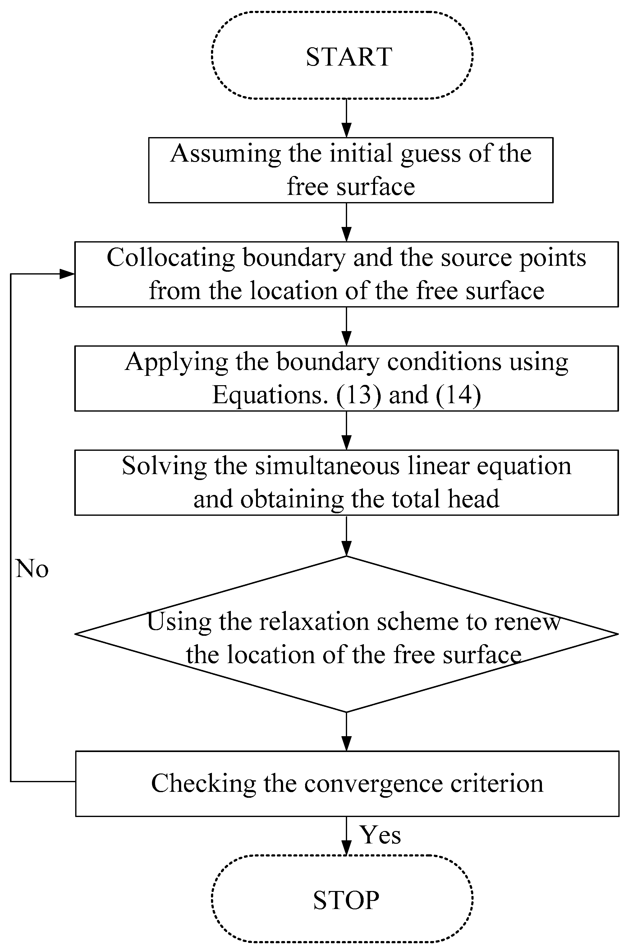
3.2. The Relaxation Scheme

As the problem of the free surface flow is nonlinear, it is necessary to introduce iterative strategies to solve the nonlinear problem. The nonlinearity of the free surface flow is rooted from the boundary conditions of the moving surface, since the governing equation is the linear Laplace equation. To obtain the location of the nonlinear free surface, the iterative method is used to generate a sequence of approximated locations of the free surface from the previous one until the termination criterion is reached. In the iterative process, the position of the boundary and the source points in the MFS must be renewed together with the free surface boundary. In 2006, Mehl [37] adopted the Picard method, which is one of the fixed-point iteration schemes for the seepage problems with the nonlinear phenomenon. Though the most successful technique for solving nonlinear problems is based on Newton’s method, it is sometimes difficult to use to obtaining the Jacobian for certain problems. As a result, the relaxation scheme based on the fixed-point iteration scheme with a relaxation factor is adopted in this study for solving the nonlinear free surface problems in the three-dimensional domain. Over-relaxation and under-relaxation factors are often used in the iteration scheme. The relaxation scheme with the under-relaxation factor is adopted in this study because it may be useful for convergence. The value of the under-relaxation factor is from 0 to 1. We used the relaxation scheme for the solutions only on the moving surface. The following equation may be obtained:

$${\tilde{h}}^{(J)}({\mathbf{x}}_k)=h^{(J-1)}({\mathbf{x}}_k)+\beta (h^{(J)}({\mathbf{x}}_k)-h^{(J-1)}({\mathbf{x}}_k)),$$

(16)

where $\beta$ is the factor of under-relaxation, and ${\tilde{h}}^{(J)}({\mathbf{x}}_k)$ is the head of the boundary point on the moving surface to be updated. After ${\tilde{h}}^{(J)}({\mathbf{x}}_k)$ is obtained, it is adopted as the guess of the head for the computation of the next iteration. In addition, the heads for the collocation points on the moving surface need to be updated using the following equation:

$$h^{(J)}({\mathbf{x}}_k)\approx {\displaystyle \sum _{j=1}^N{c}_j^{(J)}F({\mathbf{x}}_k^{(J)},{\mathbf{y}}_j^{(J)})},$$

(17)

where $J$ is the iteration counter. The iteration terminates while the following convergence criterion is achieved:

$$\epsilon =\frac{\sqrt{{\displaystyle \sum _{k=1}^{ni}(h^J({\mathbf{x}}_k)}-h^{J-1}({\mathbf{x}}_k){)}^2}}{\sqrt{{\displaystyle \sum _{k=1}^{ni}(}{h}^{J-1}({\mathbf{x}}_k){)}^2}}\le {10}^{-4},$$

(18)

where $ni$ is the collocation point number on the free surface. The flow chart of the procedure is shown in Figure 2.

4. Validation Examples

4.1. Analysis of Three-Dimensional Seepage Flow Problem

A three-dimensional problem [38] with the peanut-shaped boundary was solved. The domain, $\Omega$, is peanut-shaped, as shown in Figure 3. The boundary in three dimensions is defined as

$$\Omega =\{(x,y,z)|x=\rho (\theta )\sin \theta ,y=\rho (\theta )\sin \theta ,0\le z\le 1\},$$

(19)

where $\rho (\theta )={(\cos (2\theta )+\sqrt{1.1-{\sin }^2(2\theta )})}^{1/2}$, $0\le \theta \le 2\pi$.

The exact solution is

$$h=z\cos x\cosh y+z\sin x\sinh y.$$

(20)

To find the satisfactory source points for three-dimensional problems, we conducted a sensitivity study [39]. The boundary points are expressed as follows:

$${\mathbf{x}}_k=({\rho }_k\cos {\theta }_k,{\rho }_k\sin {\theta }_k,z_k),k=1,\dots ,Q.$$

(21)

The source points are represented by multiply a dilation parameter $\eta$ from the above equation.

$${\mathbf{y}}_l=\eta ({\rho }_l\cos {\theta }_l,{\rho }_l\sin {\theta }_l,z_l),l=1,\dots ,Q,$$

(22)

where $\eta$ is the dilation parameter for determining the positon of the source points and is greater than one. ${\theta }_k$ and ${\theta }_l$ are the azimuths. ${\rho }_k$ and ${\rho }_l$ are the radial distances. $z_k$ and $z_l$ are the vertical distances. The Dirichlet data are given from Equation (20). From Figure 4, it is significant that we obtain the best accuracy while $\eta =18$. It is also found that the maximum absolute error (MAE) can reach up to the order of ${10}^{-11}$. We conduct another example using $\eta =18$. Figure 5 depicts the computed head of the MAE to the source number. Good accuracy can be obtained after the source number greater than 1700. Figure 6 demonstrates the comparison of the head with the exact solution on the profile of $z=0.5$. We obtain accurate numerical results with the MAE in the order of ${10}^{-12}$, as shown in Figure 7.

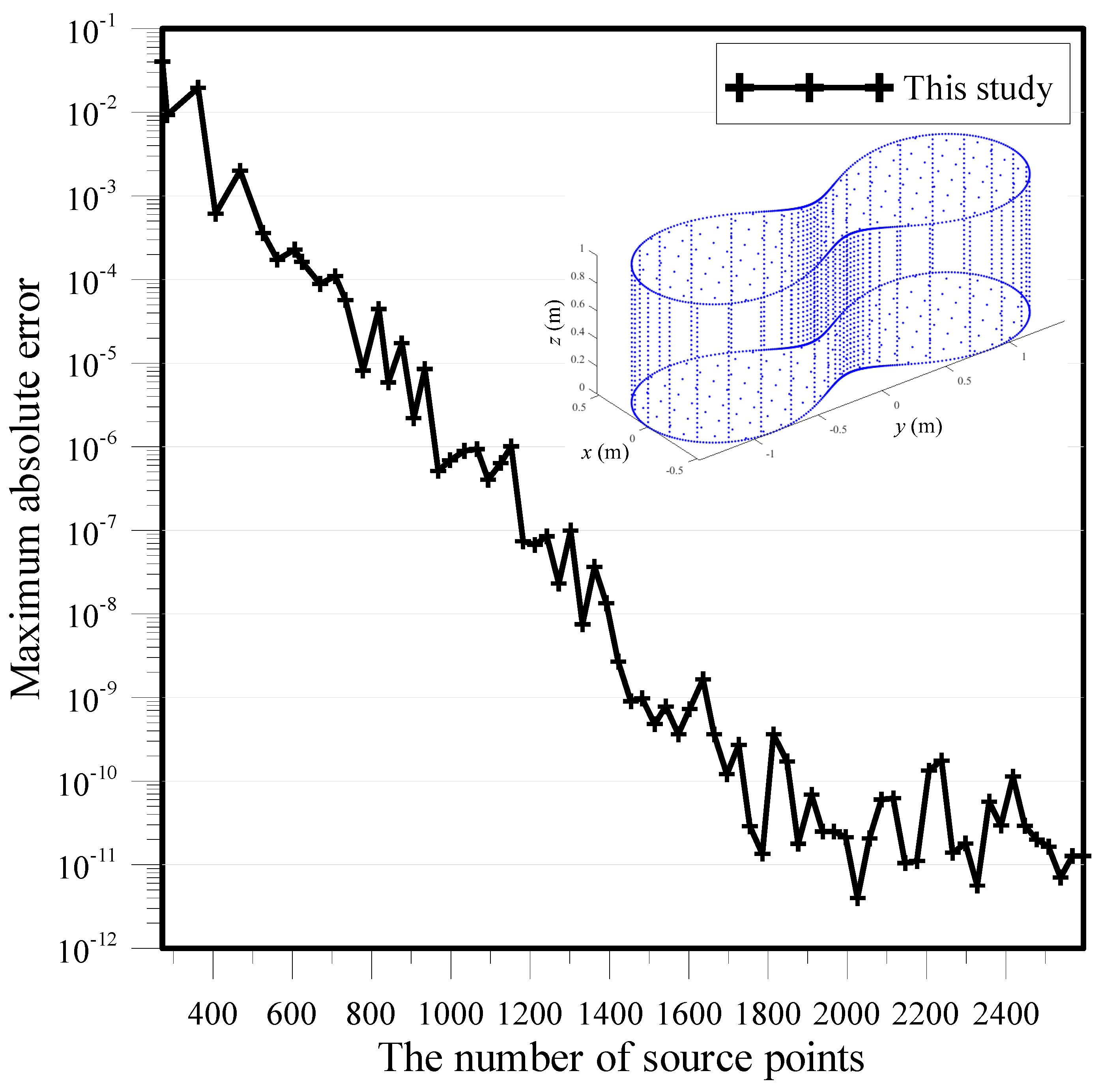
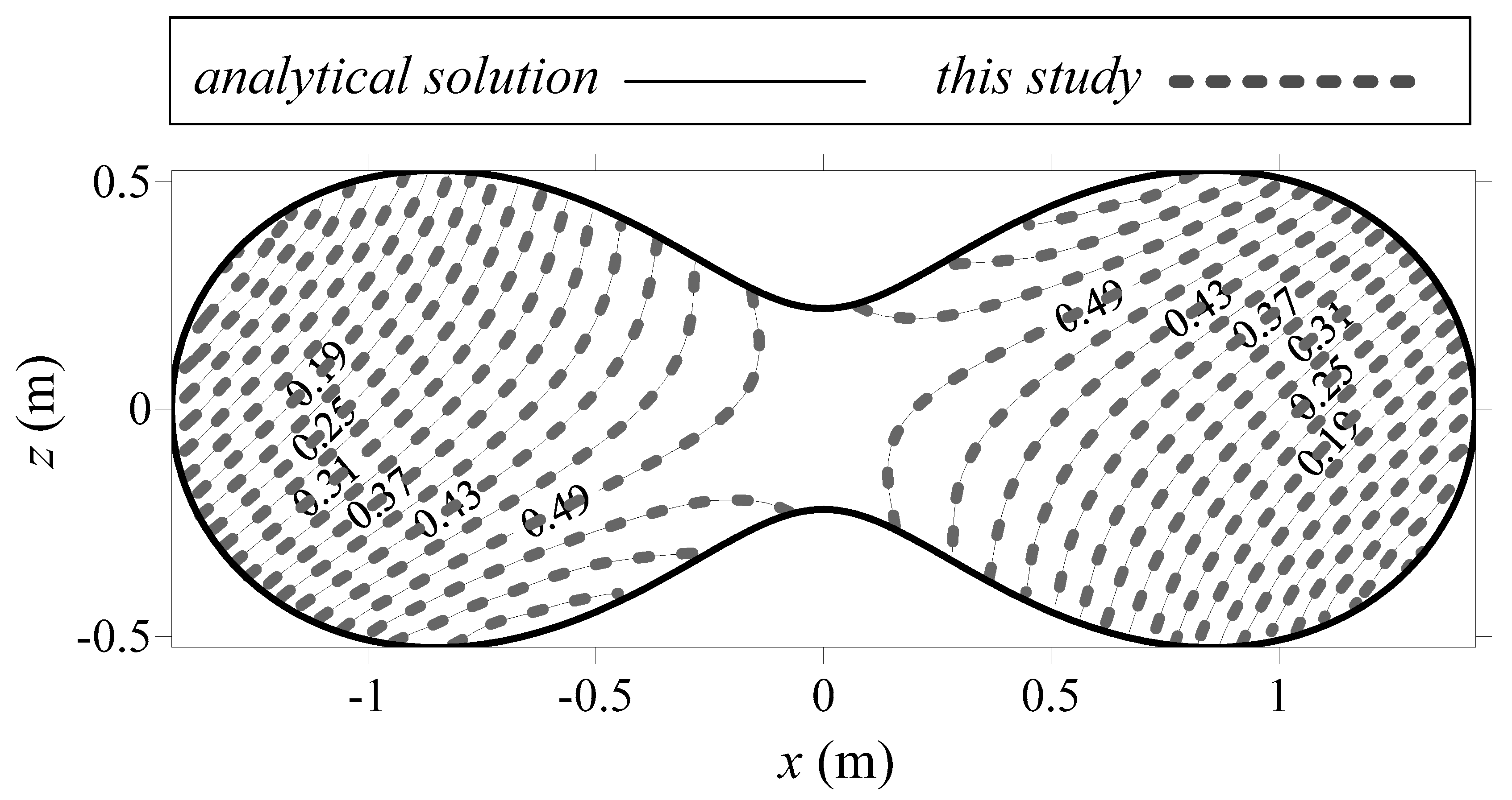
4.2. Analysis of Laminar Flow Around a Cylinder in Three Dimensions

The second example for the validation is the analysis of laminar flow around a cylinder in three dimensions, as depicted in Figure 8. The dimensions of the example are 8, 1 and 4 m in length, width and height, respectively. The radius of the cylinder at the center is 1 m. As the geometry of the problem is symmetrical, only the upper half part of the symmetry model is considered. The exact solution of the problem can be written as

$$h=e^y\cos x+e^x\sin z.$$

(23)

The Dirichlet data are from Equation (23) for the problem. As depicted in Figure 8, the boundaries of the three-dimensional laminar flow around a cylinder can be presented by ${\Gamma }_{abcd}$, ${\Gamma }_{adef}$, …, ${\Gamma }_{dfgikc}$. In this example, the dilation parameter, $\eta$, is set to be 2. In total, 3200 boundary points were collocated on the entire boundary, as demonstrated in Figure 9. To obtain the field solutions, we placed 400 points within the domain. Figure 10 depicts the head distribution of computed result versus the analytical solution. We obtain accurate numerical results with the order of ${10}^{-5}$ for the MAE, as shown in Figure 11.

5. Application of the Proposed Method

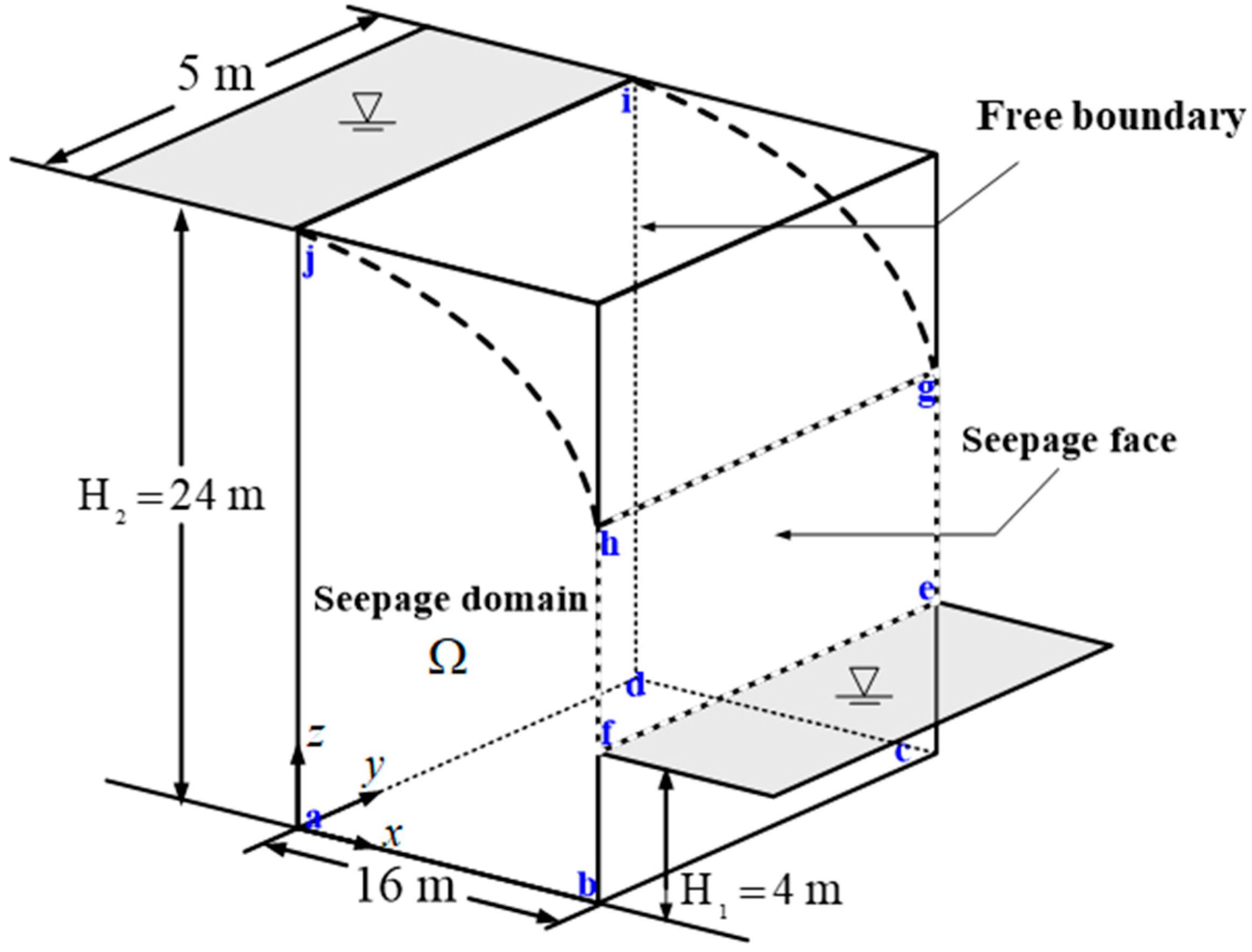
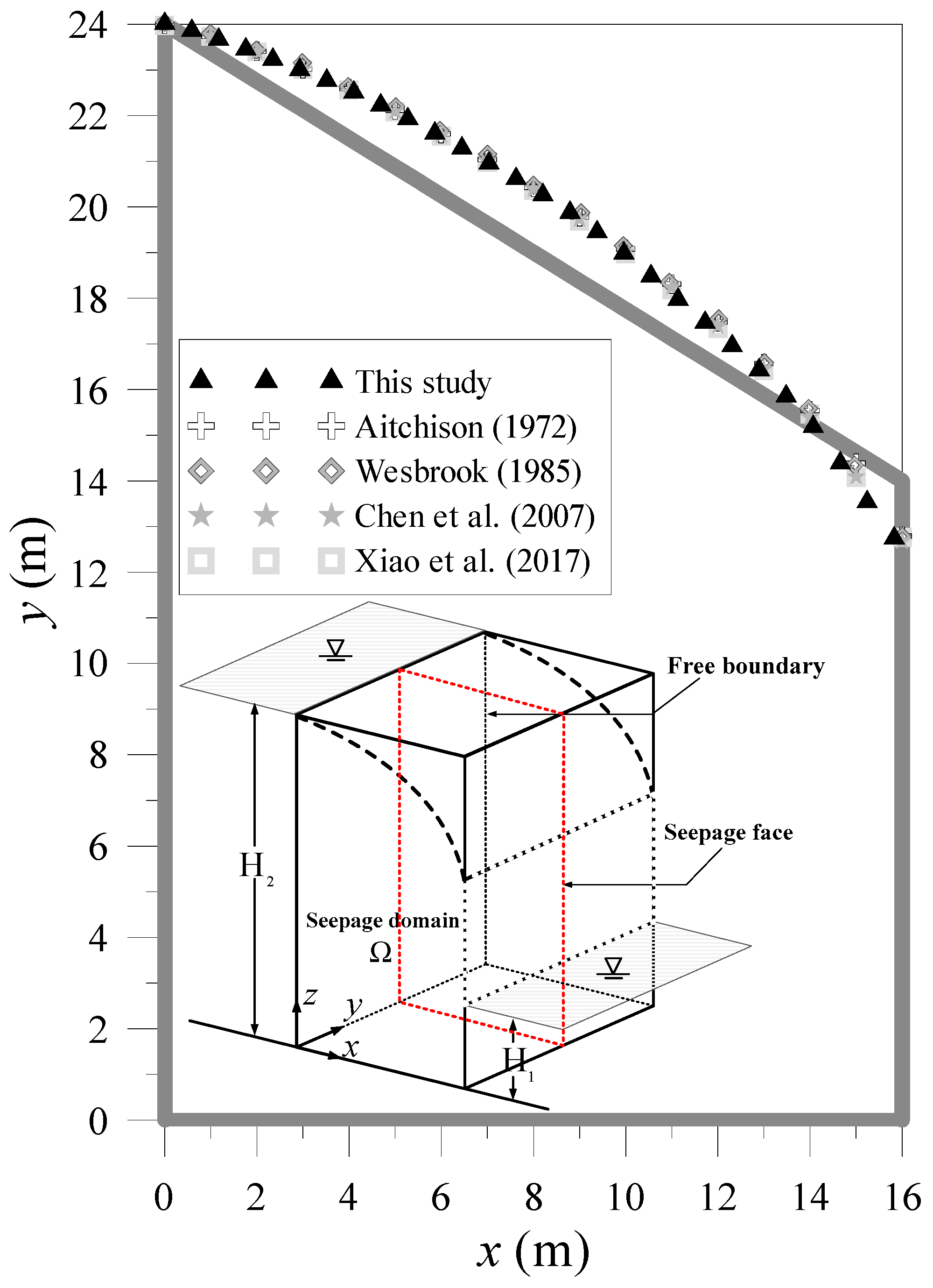
5.1. Flow Through a Rectangular Dam in Three Dimensions

The flow through a rectangular dam with a moving surface in three dimensions is presented in Figure 1. The three-dimensional moving surface is the surface of the barometric pressure and an unsaturated zone is above the moving surface. The problem is regarded as an inverse problem solved by the relaxation scheme for finding free surface. The dimensions of the example are 16, 5 and 24 m in length, width and height, respectively. In addition, the upstream water elevation ${\mathrm{H}}_2=24\mathrm{m}$ and the downstream water elevation ${\mathrm{H}}_1=4\mathrm{m}$. This example is also regarded as a typical problem which has been comprehensively studied in the past [1,40,41].

In this example, the dilation parameter $\eta$ is set to 20. In total, 6300 points were collocated on the whole boundary. The initial guess of the three-dimensional free surface is composed of 1800 boundary collocation points, as depicted in Figure 12. A total of 280 iterations were used to achieve the stopping criterion by the relaxation scheme. In order to verify the result with those from previous studies, we select the profile on $y=2.5$ and compared the computed free surface with other published studies [1,40,41], as depicted in Figure 13.

Table 1. Comparison of computed result of the separation point with those from references.

Reference	Height (m)
This study	12.75
Aitchison [40]	12.79
Chen, Hsiao, Chiu and Lee [41]	12.68
Xiao, Ku, Liu, Fan and Yeih [1]	12.84

demonstrates the comparison of the computed location of the separation point with those from references [1,40,41]. The result of the separation point is 12.75 m. We find that the computed result of the separation point is close to those from other studies.

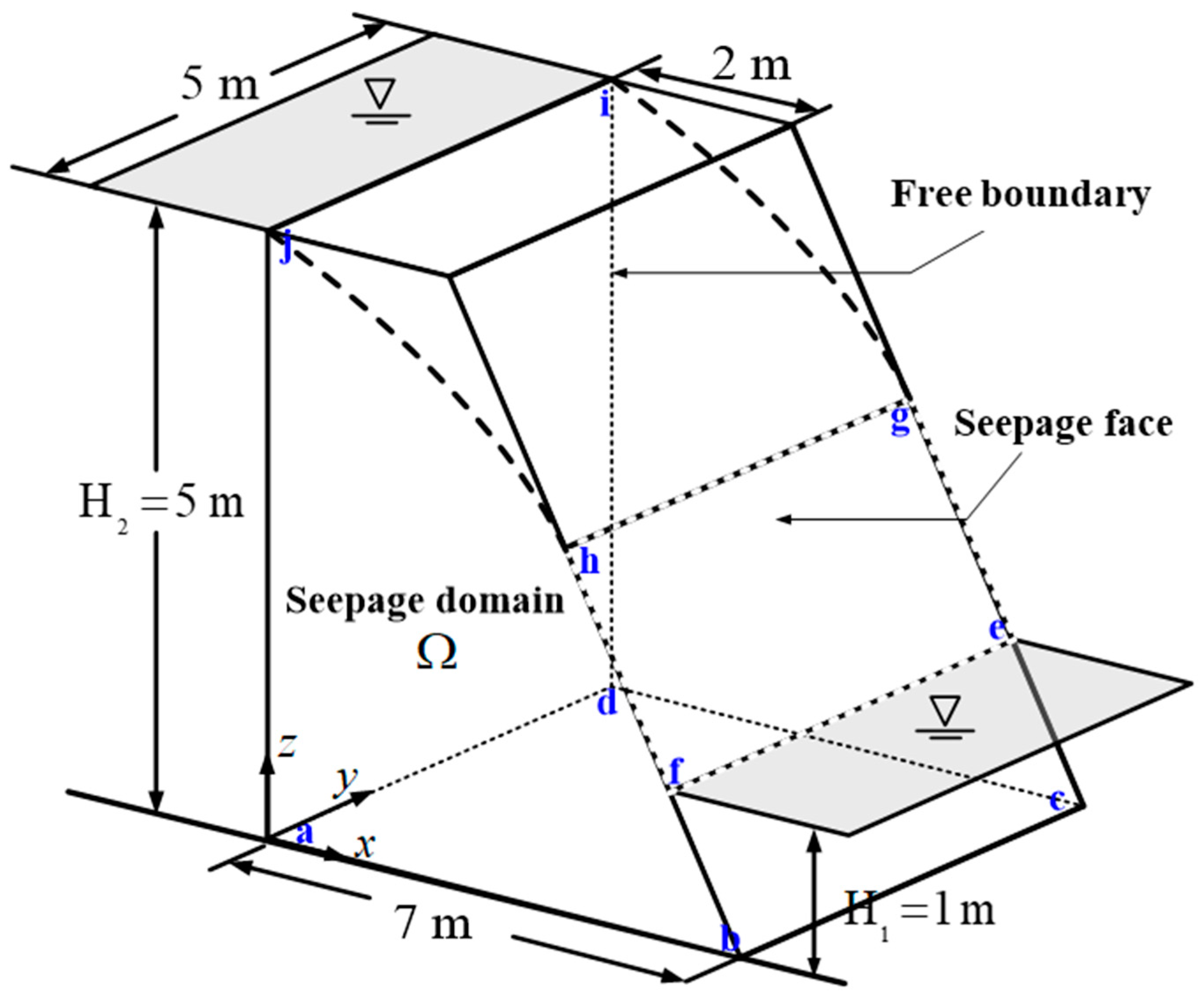
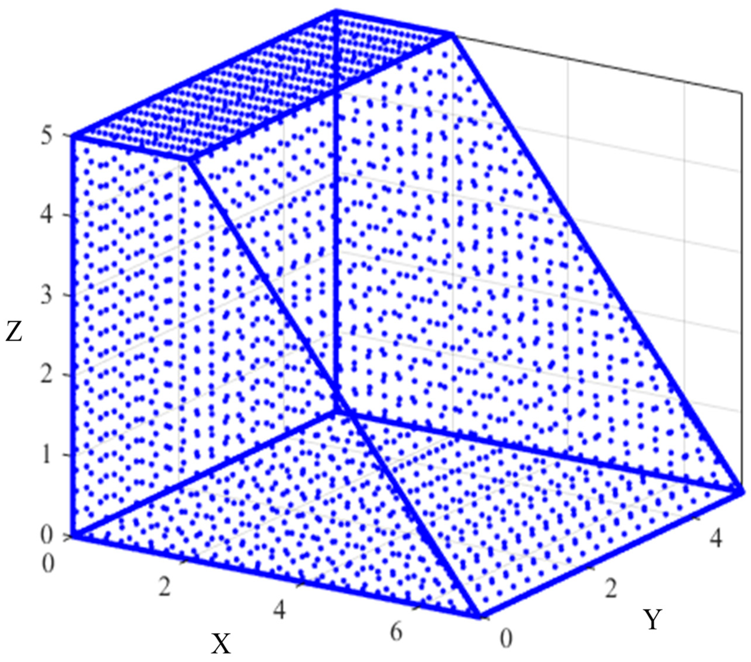
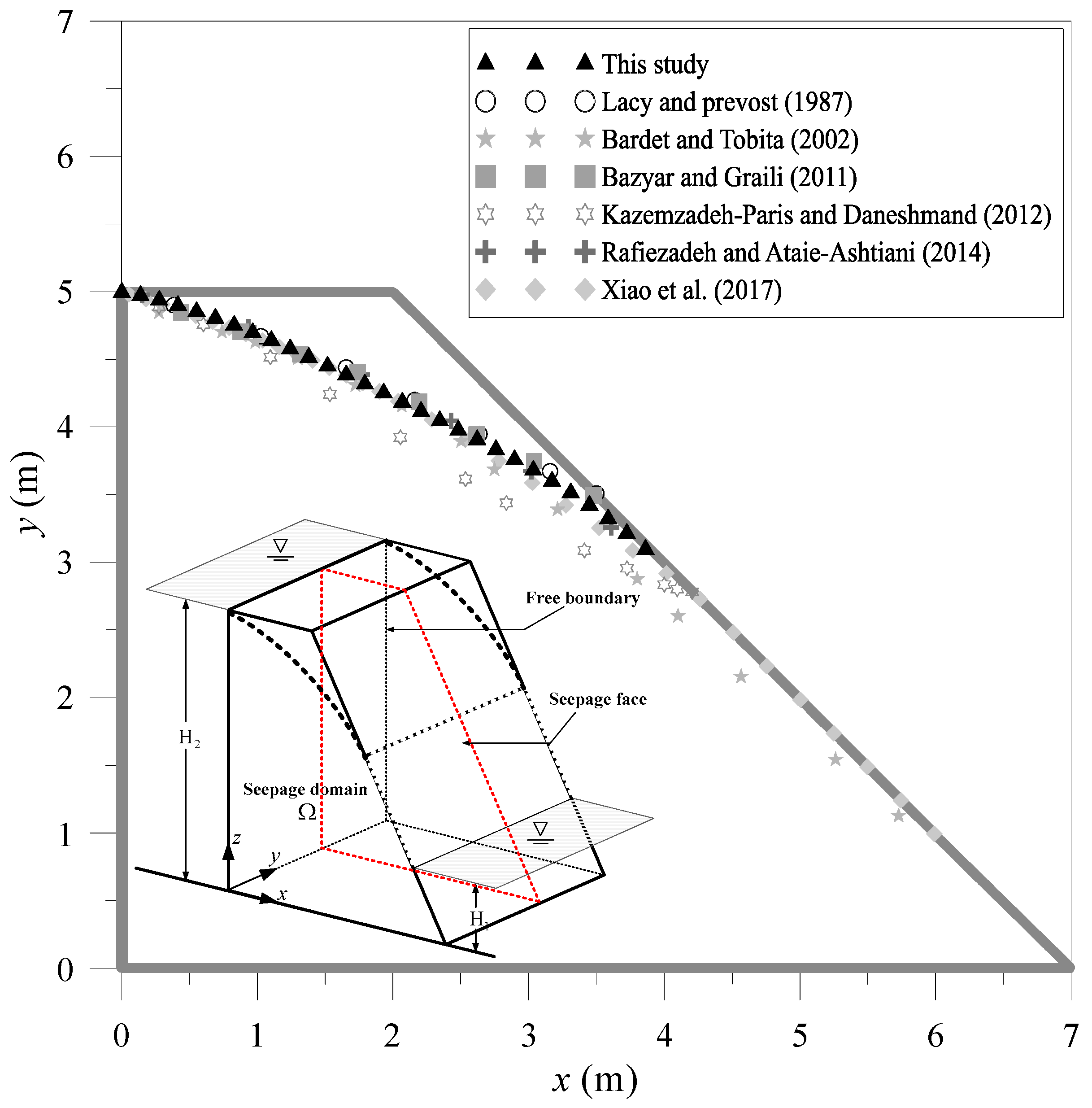
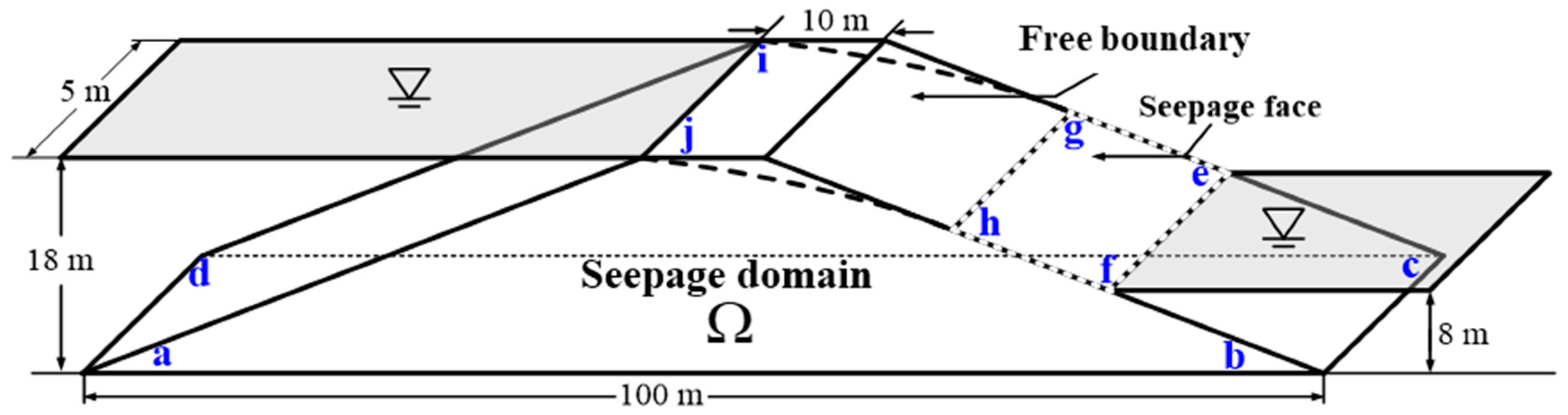
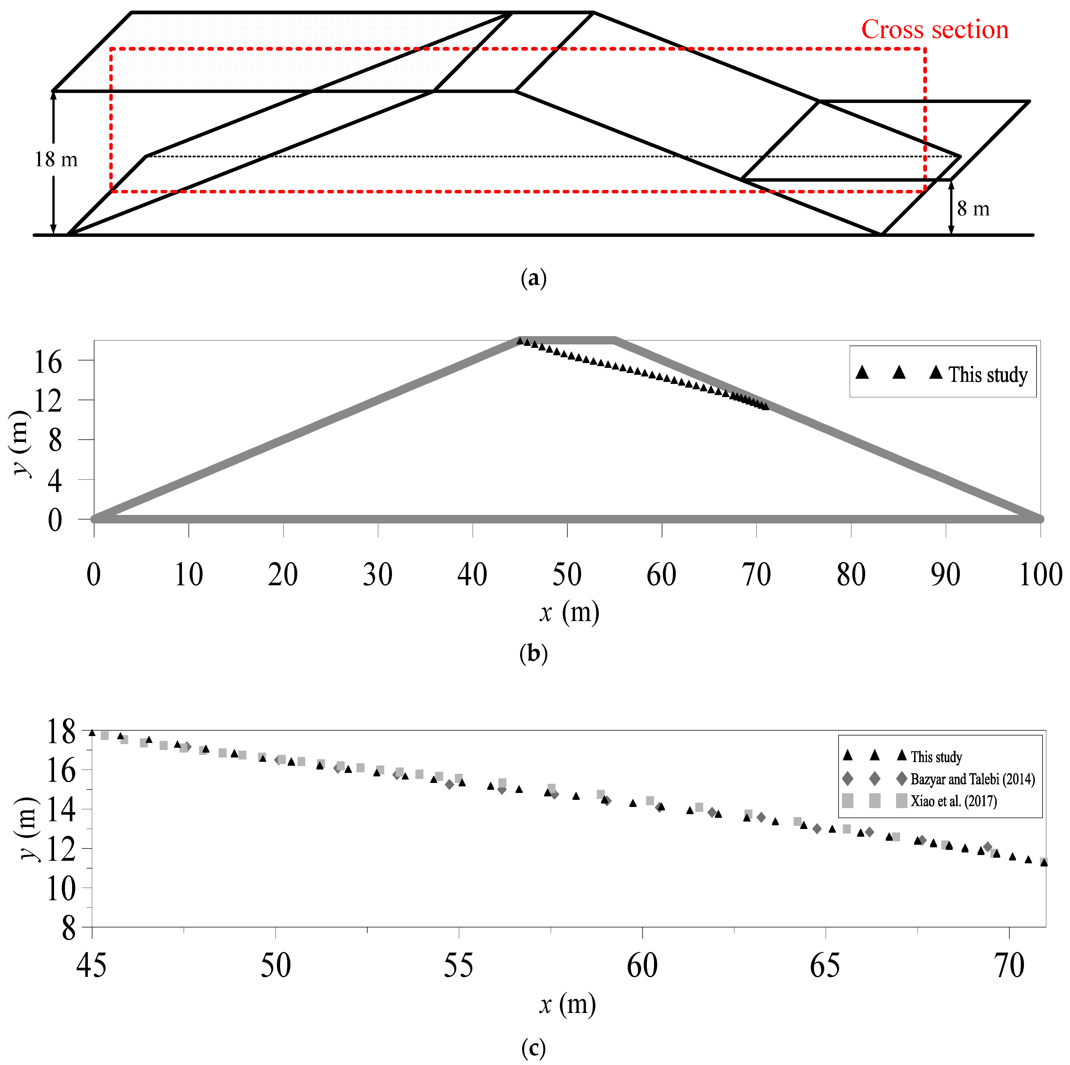
5.2. Flow Through a Trapezoidal Dam in Three Dimensions

The flow through a trapezoidal dam with a moving surface in three dimensions is presented in Figure 14. The length, width and height of the trapezoidal dam are 7, 5, and 5 m, respectively. On ${\Gamma }_{adij}$ and ${\Gamma }_{bcef}$, the Dirichlet data were assigned as ${\mathrm{H}}_2=5\mathrm{m}$ on ${\Gamma }_{adij}$ and ${\mathrm{H}}_1=1\mathrm{m}$ on ${\Gamma }_{bcef}$. The Neumann data for no flow boundary were assigned on ${\Gamma }_{abcd}$, ${\Gamma }_{abhj}$ and ${\Gamma }_{dcgi}$. On the moving surface, the following boundary conditions are given as

$$\frac{\partial h}{\partial n}=0,h=z\mathrm{on}{\Gamma }_{hgij}.$$

(24)

In this example, the dilation parameter $\eta$ was set to be 15. In total, 6300 points were collocated on the whole boundary. The initial guess of the three-dimensional free surface was composed of 1800 boundary collocation points, as depicted in Figure 15. In total, 70 iterations were used to achieve the stopping criterion by the relaxation scheme. To verify the result with those from previous studies, we selected the profile on $y=2.5$ and compared the computed free surface with others published studies [1,42,43,44,45,46], as shown in Figure 16.

5.3. Flow Through an Earth Dam in Three Dimensions

The flow through an earth dam with a moving surface in three dimensions is presented in Figure 17. The dimensions of the example are 100, 5 and 18 m in length, width and height, respectively. The Dirichlet data were assigned as ${\mathrm{H}}_2=18\mathrm{m}$ on ${\Gamma }_{adij}$ and ${\mathrm{H}}_1=8\mathrm{m}$ on ${\Gamma }_{bcef}$. The no-flow Neumann boundary condition to simulate the imperious boundary was given on ${\Gamma }_{abcd}$, ${\Gamma }_{abhj}$ and ${\Gamma }_{dcgi}$. On the moving surface, the following boundary conditions are given as

$$\frac{\partial h}{\partial n}=0,h=z\mathrm{on}{\Gamma }_{hgij}.$$

(25)

In this example, the dilation parameter $\eta$ was set to be 8. In total, 6300 points were collocated on the whole boundary. The initial guess of the three-dimensional free surface was composed of 1800 boundary collocation points, as depicted in Figure 18. In total, 150 iterations were used to achieve the stopping criterion by the relaxation scheme. To verify the result with those from previous studies, we selected the profile on $y=2.5$ and compared the computed free surface with others published studies [1,47], as shown in Figure 19.

6. Discussion

In this study, a meshless method based on the MFS for the nonlinear free surface flows in three dimensions was investigated. Since the adjustment of the mesh generation for the mesh-based methods during the iteration process is difficult, most application of the moving boundary problems are also limited in two dimensions. To model the flow problems with a free surface, the over-specified boundary conditions are assigned on the free surface boundary so that the relaxation method in conjunction with the MFS can then be solved. The advantage of the MFS is that it avoids the difficult three-dimensional mesh generation and the points are only collocated on the problem boundary. Furthermore, the proposed method may especially advantageous for dealing with three-dimensional geometric complexity including several typical dam problems. The comparison of results shows that the position of the free surface using the MFS almost identically with other methods.

7. Conclusions

This paper presents the study on solving three-dimensional free surface flow problems in arbitrary geometries using the moving boundary-type meshless method based on the MFS. The proposed method is verified and application examples are performed. The significance of the research is addressed as follows:

• The study on solving three-dimensional free surface flow problems is still limited to the conventional mesh-based method. This study presents a pioneering work using a novel moving boundary-type meshless method based on the MFS capable of solving three-dimensional free surface flow problems over arbitrary geometries. Compared to conventional mesh-based methods, the proposed method is relatively simple because the points are collocated only on the problem boundary.
• With the advantage of the boundary-type meshless method, only the collocation points on the moving surface have to be renewed during iteration for the computation of the location of the three-dimensional nonlinear free surface. It avoids the most difficult task for handling the three-dimensional geometric complexity.
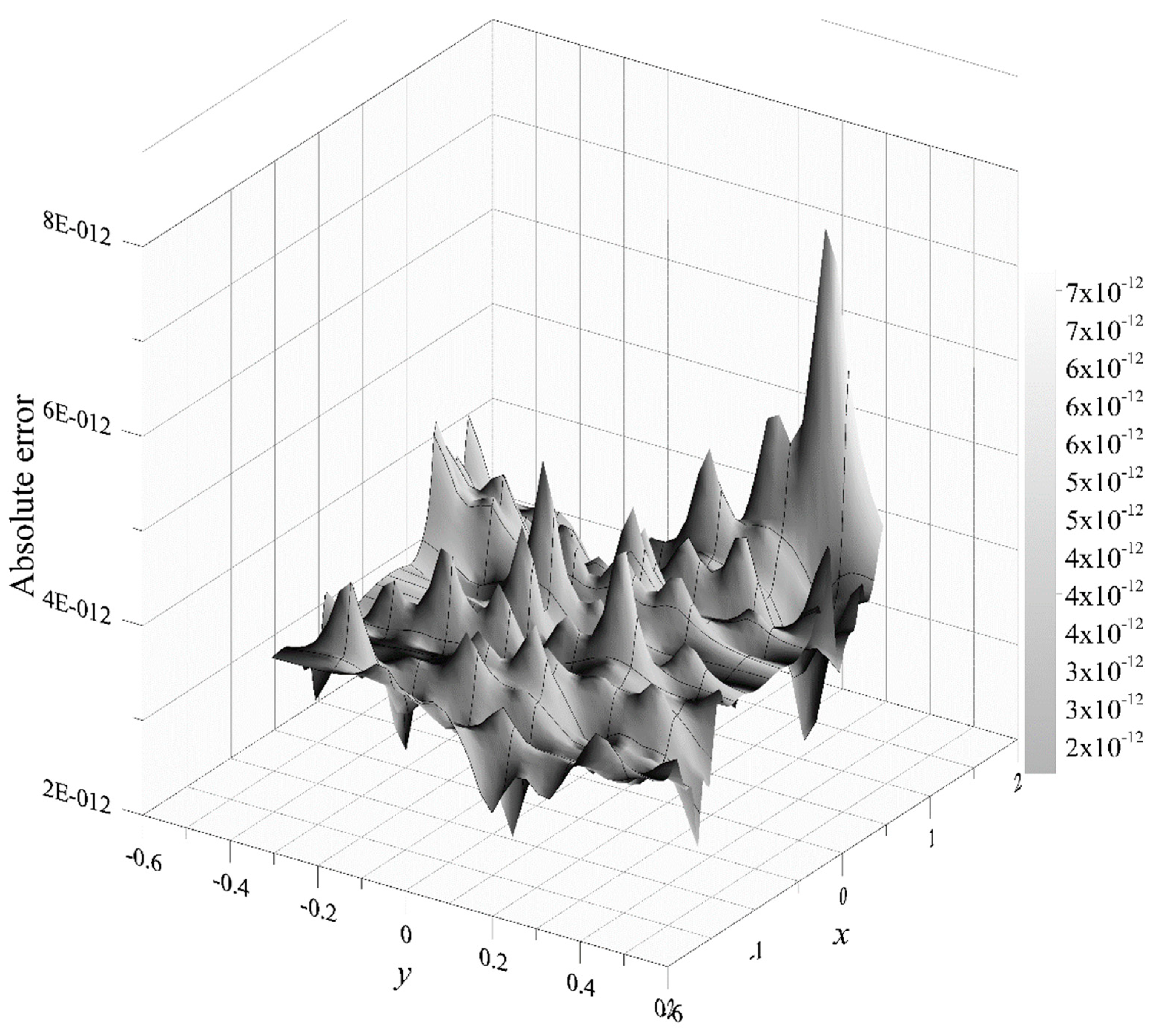
• The validation examples demonstrate that the MAE from the computed results can achieve the accuracy with the order of 10⁻¹². It is significant that our method may yield highly accurate results. The effectiveness and ease of use for solving three-dimensional nonlinear free surface flows are also revealed.
• The appearance of layered soils is often found in free surface flow problems such as the zoned embankment type dam. The anisotropic nature of layered soils is usually difficult to solve using the MFS. Further research is recommended to solve free surface flow problems in layered heterogeneous soils. It is suggested that the domain decomposition method may be an alternative to integrate with the MFS to deal with these problems in layered heterogeneous soils.
• Furthermore, the transient free surface flow problem may be a great challenge for the MFS. Several studies have been found to solve the transient heat equation using the MFS. Since the governing equation of the transient free surface flow and the transient heat conduction problems are identical, it is recommended that further research may be considered to apply the MFS for solving transient free surface flow problems.

References

1. Xiao, J.-E.; Ku, C.-Y.; Liu, C.-Y.; Fan, C.-M.; Yeih, W. On solving free surface problems in layered soil using the method of fundamental solutions. Eng. Anal. Bound. Elem. 2017, 83, 96–106. [Google Scholar]
2. Sun, G.; Lin, S.; Jiang, W.; Yang, Y. A simplified solution for calculating the phreatic line and slope stability during a sudden drawdown of the reservoir water level. Geofluids 2018, 2018. [Google Scholar] [CrossRef]
3. Cryer, C.-W. On the approximate solution of free boundary problems using finite differences. J. ACM 1970, 17, 397–411. [Google Scholar] [CrossRef]
4. Taylor, R.-L.; Brown, C.-B. Darcy flow solutions with a free surface. ASCE 1967, 93, 25–33. [Google Scholar]
5. Finn, W.D.L. Finite-element analysis of seepage through dams. ASCE 1967, 93, 41–48. [Google Scholar]
6. Neuman, S.-P.; Witherspoon, P.-A. Finite element method of analyzing steady seepage with a free surface. Water Resour. Res. 1970, 6, 889–897. [Google Scholar] [CrossRef]
7. Bathe, K.-J.; Khoshgoftaar, M.-R. Finite element free surface seepage analysis without mesh iteration. Int. J. Numer. Anal. Met. 1979, 3, 13–22. [Google Scholar] [CrossRef] [Green Version]
8. Kikuchi, N. An analysis of the variational inequalities of seepage flow by finite-element methods. Q. Appl. Math. 1977, 35, 149–163. [Google Scholar] [CrossRef] [Green Version]
9. Alt, H.-W. Numerical solution of steady-state porous flow free boundary problems. Numer. Math. 1980, 36, 73–98. [Google Scholar] [CrossRef]
10. Oden, J.-T.; Kikuchi, N. Recent advances: Theory of variational inequalities with applications to problems of flow through porous media. Int. J. Eng. Sci. 1980, 18, 1173–1284. [Google Scholar] [CrossRef]
11. Desai, C.-S.; Li, G.-C. A residual flow procedure and application for free surface flow in porous media. Adv. Water Resour. 1983, 6, 27–35. [Google Scholar] [CrossRef]
12. Westbrook, D.-R. Analysis of inequalities and residual flow procedures and an iterative scheme for free surface seepage. Int. J. Numer. Meth. Eng. 1985, 21, 1791–1802. [Google Scholar] [CrossRef]
13. Brezis, H.; Kinderlehrer, D.; Stampacchia, G. Sur une Nouvelle Formulation du Probleme de L’ecoulement a Travers une Digue; Serie A; C. R. Academie des Sciences: Paris, France, 1978. [Google Scholar]
14. Cheng, Y.-M.; Tsui, Y. An efficient method for the free surface seepage flow problems. Comput. Geotech. 1993, 15, 47–62. [Google Scholar] [CrossRef]
15. Ji, C.-N.; Wang, Y.-Z.; Shi, Y. Application of modified EP method in steady seepage analysis. Comput. Geotech. 2005, 32, 27–35. [Google Scholar] [CrossRef]
16. Fukuchi, T. Numerical analyses of steady-state seepage problems using the interpolation finite difference method. Soils Found. 2016, 56, 608–626. [Google Scholar] [CrossRef]
17. Wu, C.-P.; Lin, C.-H.; Chiou, Y.-J. Multi-region boundary element analysis of unconfined seepage problems in excavations. Comput. Geotech. 1996, 19, 75–96. [Google Scholar] [CrossRef]
18. Tsay, R.-J.; Chiou, Y.-J.; Cheng, T.-C. Boundary element analysis for free surface of seepage in earth dams. J. Chin. Inst. Eng. 1997, 20, 95–101. [Google Scholar] [CrossRef]
19. Neuman, S.-P.; Witherspoon, P.-A. Variational principles confined and unconfined flow of ground water. Water Resour. Res. 1970, 6, 1376–1382. [Google Scholar] [CrossRef]
20. Athani, S.-S.; Shivamanth; Solanki, C.-H.; Dodagoudar, G.-R. Seepage and stability analyses of earth dam using finite element method. Aquat. Procedia 2015, 4, 876–883. [Google Scholar] [CrossRef]
21. Ahmed, A.-A. Stochastic analysis of free surface flow through earth dams. Comput. Geotech. 2009, 36, 1186–1190. [Google Scholar] [CrossRef]
22. Xiao, J.-E.; Ku, C.-Y.; Huang, W.-P.; Su, Y.; Tsai, Y.-H. A novel hybrid boundary-type meshless method for solving heat conduction problems in layered materials. Appl. Sci. 2018, 8, 1887. [Google Scholar] [CrossRef]
23. Liu, C.-S. Improving the ill-conditioning of the method of fundamental solutions for 2D Laplace equation. CMES-Comput. Model. Eng. 2009, 851, 1–17. [Google Scholar]
24. Tsai, C.-C.; Young, D.-L. Using the method of fundamental solutions for obtaining exponentially convergent Helmholtz eigensolutions. CMES-Comput. Model. Eng. 2013, 94, 175–205. [Google Scholar]
25. Liu, C.-S. The method of fundamental solutions for solving the backward heat conduction problem with conditioning by a new post-conditioner. Numer. Heat Transf. B-Fund. 2011, 60, 57–72. [Google Scholar] [CrossRef]
26. Fan, C.-M.; Chen, C.-S.; Monroe, J. The method of fundamental solutions for solving convection-diffusion equations with variable coefficients. Adv. Appl. Math. Mech. 2009, 1, 215–230. [Google Scholar]
27. Li, M.; Chen, C.-S.; Karageorghis, A. The MFS for the solution of harmonic boundary value problems with non-harmonic boundary conditions. Comput. Math. Appl. 2013, 66, 2400–2424. [Google Scholar] [CrossRef]
28. Kupradze, V.-D.; Aleksidze, M.-A. The method of functional equations for the approximate solution of certain boundary value problems. USSR Comput. Math. Math. Phys. 1964, 4, 82–126. [Google Scholar] [CrossRef]
29. Young, D.-L.; Chiu, C.-L.; Fan, C.-M.; Tsai, C.-C.; Lin, Y.-C. Method of fundamental solutions for multidimensional Stokes equations by the dual-potential formulation. Eur. J. Mech. B/Fluids 2006, 25, 877–893. [Google Scholar] [CrossRef]
30. Marin, L. Treatment of singularities in the method of fundamental solutions for two-dimensional Helmholtz-type equations. Appl. Math. Model. 2010, 34, 1615–1633. [Google Scholar] [CrossRef]
31. Bello, N.; Alkali, A.-J.; Roko, A. A fixed point iterative method for the solution of two-point boundary value problems for a second order differential equations. Alexandria Eng. J. 2017, 57, 2515–2520. [Google Scholar] [CrossRef]
32. Huang, N.; Ma, C. Convergence analysis and numerical study of a fixed-point iterative method for solving systems of nonlinear equations. Sci. World J. 2014, 2014, 1–10. [Google Scholar] [CrossRef]
33. Kumar, M.; Singh, A.-K.; Srivastava, A. Various Newton-type iterative methods for solving nonlinear equations. J. Egypt. Math. Soc. 2013, 21, 334–339. [Google Scholar] [CrossRef] [Green Version]
34. Jin, S.; Xin, Z. The relaxation schemes for systems of conservation laws in arbitrary space dimensions. Commun. Pure Appl. Math. 1995, 48, 235–276. [Google Scholar] [CrossRef] [Green Version]
35. Aregba-Driollet, D.; Natalini, R. Convergence of relaxation schemes for conservation laws. Appl. Anal. 1996, 61, 163–193. [Google Scholar] [CrossRef] [Green Version]
36. Aregba-Driollet, D.; Natalini, R. Discrete kinetic schemes for multidimensional systems of conservation laws. Siam J. Numer. Anal. 2000, 37, 1973–2004. [Google Scholar] [CrossRef]
37. Mehl, S. Use of Picard and Newton iteration for solving nonlinear groundwater flow equations. Groundwater 2006, 44, 583–594. [Google Scholar] [CrossRef] [PubMed]
38. Ku, C.-Y.; Kuo, C.-L.; Fan, C.-M.; Liu, C.-S.; Guan, P.-C. Numerical solution of three-dimensional Laplacian problems using the multiple scale Trefftz method. Eng. Anal. Bound. Elem. 2015, 50, 157–168. [Google Scholar] [CrossRef]
39. Chen, C.-S.; Karageorghis, A.; Li, Y. On choosing the location of the sources in the MFS. Numer. Algorithms 2016, 72, 107–130. [Google Scholar] [CrossRef]
40. Aitchison, J. Numerical Treatment of a Singularity in a Free Boundary Problem; Royal Society of London: London, UK, 1972; pp. 573–580. [Google Scholar]
41. Chen, J.-T.; Hsiao, C.-C.; Chiu, Y.-P.; Lee, Y.-T. Study of free surface seepage problems using hypersingular equations. Comm. Numer. Meth. Eng. 2007, 23, 755–769. [Google Scholar] [CrossRef]
42. Bardet, J.-P.; Tobita, T. A practical method for solving free-surface seepage problems. Comput. Geotech. 2002, 29, 451–475. [Google Scholar] [CrossRef]
43. Rafiezadeh, K.; Ataie-Ashtiani, B. Transient free-surface seepage in three-dimensional general anisotropic media by BEM. Eng. Anal. Bound. Elem. 2014, 46, 51–66. [Google Scholar] [CrossRef]
44. Lacy, S.-J.; Prevost, J.-H. Flow through porous media: A procedure for locating the free surface. Int. J. Numer. Anal. Met. 1987, 11, 585–601. [Google Scholar] [CrossRef]
45. Bazyar, M.-H.; Graili, A. A practical and efficient numerical scheme for the analysis of steady state unconfined seepage flows. Int. J. Numer. Anal. Met. 2011, 36, 1793–1812. [Google Scholar] [CrossRef]
46. Kazemzadeh-Parsi, M.-J.; Daneshmand, F. Unconfined seepage analysis in earth dams using smoothed fixed grid finite element method. Int. J. Numer. Anal. Met. 2011, 36, 780–797. [Google Scholar] [CrossRef]
47. Bazyar, M.-H.; Talebi, A. Locating the free surface flow in porous media using the scaled boundary finite-element method. Int. J. Chem. Eng. Appl. 2014, 5, 155–160. [Google Scholar] [CrossRef]
Figure 1. Three-dimensional nonlinear free surface flow through a dam.
Applsci 09 01715 g001
Figure 2. Flow chart of solving nonlinear free surface using the relaxation scheme.
Applsci 09 01715 g002
Figure 3. A three-dimensional peanut-shaped domain for the analysis. (a) Boundary collocation points and (b) source points.
Applsci 09 01715 g003
Figure 4. Maximum absolute error (MAE) versus the order of η .
Applsci 09 01715 g004
Figure 5. MAE versus the source number.
Applsci 09 01715 g005
Figure 6. Comparison of the computed head with the exact solution on profile z = 0.5 .
Applsci 09 01715 g006
Figure 7. Absolute error of example 4.1.
Applsci 09 01715 g007
Figure 8. Laminar flow around a cylinder in three dimensions.
Applsci 09 01715 g008
Figure 9. Collocation points on the three-dimensional boundary.
Applsci 09 01715 g009
Figure 10. Comparison of head distribution of the method of fundamental solutions (MFS) with the analytical solution on profile y = 0.5 .
Applsci 09 01715 g010
Figure 11. Absolute error of example 4.2.
Applsci 09 01715 g011
Figure 12. Collocation points on the three-dimensional boundary.
Applsci 09 01715 g012
Figure 13. Comparison of the computed results for a rectangular dam on profile y = 2.5 .
Applsci 09 01715 g013
Figure 14. Flow through a trapezoidal dam in three dimensions.
Applsci 09 01715 g014
Figure 15. Collocation points on the three-dimensional boundary.
Applsci 09 01715 g015
Figure 16. Comparison of the computed results for a trapezoidal dam on profile y = 2.5 .
Applsci 09 01715 g016
Figure 17. Flow through an earth dam in three–dimensions.
Applsci 09 01715 g017
Figure 18. Collocation points on the three-dimensional boundary.
Applsci 09 01715 g018
Figure 19. (a) The selected cross section, (b) computed free surface of an earth dam on profile y = 2.5 and (c) result comparison on profile y = 2.5 .
Applsci 09 01715 g019