Gaussian Process-Integrated State Space Model for Continuous Joint Angle Prediction from EMG and Interactive Force in a Human-Exoskeleton System

Abstract

As one of the most direct indicators of the transparency between a human and an exoskeleton, interactive force has rarely been fused with electromyography (EMG) in the control of human-exoskeleton systems, the performances of which are largely determined by the accuracy of the continuous joint angle prediction. To achieve intuitive and naturalistic human intent learning, a state space model (SSM) for continuous angle prediction of knee joint is developed. When the influence of the interactive force is often ignored in the existing models of human-exoskeleton systems, interactive force is applied as the measurement model output of the proposed SSM, and the EMG signal is used as the state model input signal to indicate muscle activation. The forward dynamics of joint motion and the human-machine interaction mechanism, i.e., the biomechanical interpretations of the interactive force generation mechanism, are derived as the bases for the state model and measurement model based on Hill’s muscle model and semiphenomenological (SP) muscular model, respectively. Gaussian process (GP)-based nonlinear autoregressive with the exogenous inputs (NARX) model and back-propagation neural network (BPNN) are applied to provide better adaptivity for the SSM in practical applications. Corresponding experimental results demonstrate the validity and superiority of the method.

1. Introduction

Modern robots, such as rehabilitation robots, try to actively interact with human partners towards achieving a common task. This gives rise to the emerging field of research named human robot interaction (HRI), aiming at maximizing the performance, efficiency, and applicability of coupled human–robot systems [1]. It can be defined as “a field of study dedicated to understanding, designing, and evaluating robotic systems for use by or with humans” [2]. The system performance, however, is largely limited by the output of human intent learning and prediction [3]. In many human-robot systems, continuous human motion intents instead of a limited number of classified motion patterns have to be identified and further reconstructed as control commands to the robot so that the robot could match human motion intents and perform efficient assistances [4]. Thus, how to determine the human motion intent in terms of continuous joint angle has become the key issue. Two main related problems remain: one is the choice of the learning model for continuous joint angle prediction, the other is the selection of input signals that could reflect both the human motion dynamics and the human-robot interaction state well.

As for the modelling methods for the forward dynamics of human neuromusculoskeletal system, one choice is the application of phenomenological or semi-phenomenological models. Clear biomechanical interpretations can be found in these kinds of models. Although most of the existing models, such as the model proposed by Zajac [5] and Zahalak [6,7], are based on the phenomenological models derived from Hill’s work [8] or the more complex biophysical model of Huxley [9], the transformation from muscle activation to muscle force and human kinematics has not been fully understood yet. In addition, the determination of muscle geometry, such as the muscle-tendon moment arm, is especially difficult for a living person and thus makes the estimation prone to error [10,11]. Problems also exist associated with the application of phenomenological models when the workload of the model parameter identification for each subject is extremely heavy [12,13].

The other approach that bypasses the above problems and limitations is to use machine learning methods. Moreover, with the fast development of artificial intelligence, artificial neural networks (ANNs) are now widely applied in the control of human-exoskeleton systems [1]. In addition, the Gaussian process (GP) is also receiving more attention in the field [14,15,16]. The GP model has superior flexibility when the parameters that directly determine the model performance can be adjusted through learning [17,18]. As for the mapping structure, one widely applied approach is to map muscle activation or neural signals to the joint angle [19]. When the history of the movements reflects the inherent dynamics of human motion [20], joint angle could also be predicted using autoregressive models. To combine the advantages of both and achieve continuous, intuitive and naturalistic understanding of human motion intent, nonlinear autoregressive with exogenous inputs (NARX) would be a better choice and has begun to be applied in the field of joint angle prediction [4,21,22]. Its application combines the non-linear spatio-temporal correlation structure of natural human movements with muscle-driven control signals to exploit the best of both worlds [23].

However, such approaches treat the entire central nervous system as a black box with no biomechanical interpretations. Thus, the application is still a matter of great debate.

The ideal solution to such a contradiction should be one model that not only integrates the state-of-art machine learning techniques that provide good adaptivity for practical applications, but also has corresponding biomechanical interpretations. When the state model and measurement model of state space model (SSM) could be used to interpret the related biomechanical mechanisms, the SSM, which also integrates GP and ANN, may be the promising choice.

For the input signal selection, electromyography (EMG) signals which reflect the muscle activation have been widely utilized in the fields of joint angle learning and prediction [19,24]. The EMG signal provides easy access to physiological processes that cause the muscle to generate force and produce movement. Different from intramuscular EMG which uses a fine needle electrode inserted into the muscle, surface EMG (sEMG) is more commonly used due to its outstanding characters including noninvasiveness and safety [25,26]. As the quality of sEMG signals is very sensitive to muscle fatigue, sweat, and changing electrode characteristics, a proper processing method is needed and the application of on-line learning approaches, such as the GP and ANN as just introduced, would be preferred. In addition, sEMG signals are also used as the measurement output in SSMs for human joint angle prediction, such as the redundant subsectors of the sEMG-vector [4] and other extracted EMG features, including waveform length (WL) and zero crossing (ZC) [27]. Meanwhile, interactive force, which is a direct end-effector reflection in human-exoskeleton systems, can be regarded as an important indicator of transparency between a human and robot [28,29]. Although the fusion of EMG and force would improve the performance of joint angle prediction, interactive force has rarely been used in combination with EMG signals in joint angle prediction [30]. More importantly, how the interactive force works in the human-exoskeleton system model, i.e., its biomechanical generation mechanism, is often ignored. Thus, the influence of the interactive force on the human-exoskeleton system is always overlooked.

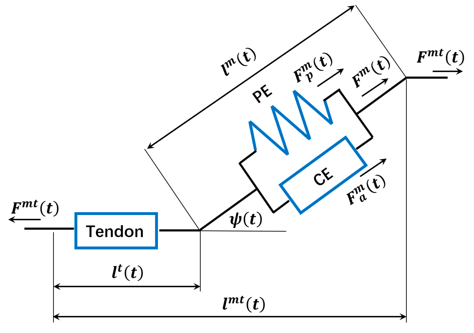
The motivation of this paper is to develop a GP-integrated SSM for continuous joint prediction and to provide biomechanical interpretations for its state model and measurement model in human-exoskeleton integrated applications. To the best of our knowledge, the interactive force has rarely been used in combination with EMG signals in the continuous joint prediction of human-exoskeleton systems. In the proposed model, interactive force is applied as the measurement model output and the EMG signal is used as the state model input to indicate muscle activation. Hill’s muscle model and semi-phenomenological (SP) model [31] are adopted to acquire the forward dynamics of joint motion for the state model and the human-machine interaction mechanism interpretation for the measurement model, respectively. In practical applications, the GP-based NARX model and back propagation neural network (BPNN) are applied to provide better flexibility and adaptivity. Compared with the existing SSMs for continuous joint angle prediction [4,27], our main contributions lie in three aspects. First, interactive force is fused with the EMG signal in the SSM instead of using extracted EMG signal features alone. When the impacts of interactive force on the human-exoskeleton system are considered, the performance of joint angle prediction would improve. Second, in addition to the use of machine learning techniques, Hill’s muscle model and SP model are used to derive the biomechanical mechanisms for the state model and measurement model of the proposed SSM. Third, as a non-parametric model, GP is integrated with traditional BPNN to combine the relative strengths of both the parametric model and non-parametric model. Corresponding experimental results demonstrate the validity and superiority of the method.

2. Forward Dynamics and Human Exoskeleton Interaction Mechanism Interpretation of The Knee Joint

2.1. Hill’s Muscle Model Based Forward Dynamics of the Knee Joint

Most of the existing approaches [6,7,9] studying the forward dynamics of human movement are based on the phenomenological models derived from Hill’s muscle model [8] and its extension proposed by Zajac [5]. The corresponding muscle-tendon unit is illustrated in Figure 1. Here, the human knee joint is chosen as our research object.

2.1.1. Muscle Contraction Dynamics

According to Hill’s muscle model [5,8], the muscle-tendon force $F^{mt}$ consists of two elements: a contractile element producing the active muscle force $F_A^m$ and a parallel elastic element producing the passive force $F_P^m$ [27]. Thus, the generated muscle-tendon force is usually developed as follows [10,11,12,32]:

$$F^{mt}=\left[F_A^m+F_P^m\right]cos\varphi =\left[f_A\left(l\right)f_V\left(v\right)a\left(k\right)+f_P\left(l\right)\right]F_0^{m}cos\varphi$$

(1)

where $f_A\left(l\right)$ is the normalized active force-length relationship of the contractile element, $f_V\left(v\right)$ corresponds to the normalized force-velocity relationship of the contractile element, $f_P\left(l\right)$ refers to the normalized passive elastics force-length relation, $a\left(k\right)$ is the activation of the muscle fiber in the k-th time step, $F_0^m$ is the maximum isometric muscle force. $l=l^m/l_0^m$ is the normalized muscle fiber length where $l^m$ is the fiber length and $l_0^m$ is the optimum fiber length, $v=v^m/v_0^m$ is the normalized muscle fiber velocity where $v^m$ is the muscle contraction velocity and $v_0^m$ is the maximum muscle contraction velocity, $\varphi$ is the pennation angle.

The nonlinearly of $f_A\left(l\right)$, $f_V\left(v\right)$ and $f_P\left(l\right)$ leads to great difficulties for the model to be applied in practical engineering. Thus, some simplifications have to be made [10,33]:

$$f_A\left(l\right)=\{\begin{array}{c}{q}_0+q_{1}l+q_2{l}^2\\ 0\end{array},\begin{array}{c}0.5\le l\le 1.5\\ otherwise\end{array}$$

$$f_P\left(l\right)=e^{10l-15}$$

$$f_V\left(v\right)=1$$

where $q_0,q_1$ and $q_2$ are set to be constants [27].

2.1.2. Musculoskeletal Geometry

Based on geometrical relations illustrated in Figure 1, the muscle-tendon length $l^{mt}$ can be represented as

$$l^{mt}=l^t+l^{m}cos\varphi$$

(2)

where $l^t$ is the tendon length. In (1) and (2), the physiological parameters, including $l^t,l_0^m,F_0^m$ and $\varphi$, can all be set as constants.

Meanwhile, muscle-tendon length $l^{mt}$ can be expressed by a polynomial of the joint angle [34]. Here, a first-order polynomial is used for simplification:

$$l^{mt}=b_0+b_1\theta$$

(3)

where $\theta$ is the angle of the knee joint, $b_0$ and $b_1$ are both fitting constants.

Thus, it is easy to obtain the expression of muscle fiber length $l$ about the joint angle $\theta$ when combining (2) and (3)

$$l=\frac{b_1}{l_0^{m}cos\varphi }\theta +\frac{b_0-l^t}{l_0^{m}cos\varphi }$$

(4)

The moment arm $r$ of the muscle associated with the joint movement can be calculated using the tendon displacement method [5,34]:

$$r=\frac{\partial l^{mt}\left(\theta \right)}{\partial \theta }=b_1$$

(5)

The corresponding moment $\mathsf{\tau }$ can then be expressed as:

$$\mathsf{\tau }=F^{mt}r$$

(6)

2.1.3. Joint Motion Model

Based on the muscle contraction dynamics and the musculoskeletal geometry, the joint motion model can be described as:

$$\ddot{\theta }{I}_e=\mathsf{\tau }-{\mathsf{\tau }}_{ex}$$

(7)

where $I_e$ is the moment of inertia of the knee joint, ${\mathsf{\tau }}_{ex}$ is a combination of the external torque and the calf gravity torque, the maximum value of which is denoted as ${\mathsf{\tau }}_{ex\_max}$. Their relation is as follows:

$${\mathsf{\tau }}_{ex}={\mathsf{\tau }}_{ex\_max}sin\theta$$

(8)

Given that in practical control processes both the angular velocity and acceleration are calculated in the discrete way through numerical methods, they are defined as follows when the sampling time is set as $T_s$:

$$\{\begin{array}{c}{\dot{\theta }}_k=\frac{1}{T_s}\left({\theta }_{k+1}-{\theta }_k\right)\\ {\ddot{\theta }}_k=\frac{1}{T_s}\left({\dot{\theta }}_{k+1}-{\dot{\theta }}_k\right)\end{array}$$

Consequently, when combining (6), (7) and (8), the joint motion model can be expressed as follows:

$$\frac{1}{T_s}\left({\dot{\theta }}_{k+1}-{\dot{\theta }}_k\right)={\ddot{\theta }}_k=\frac{1}{I_e}\left(\mathsf{\tau }-{\mathsf{\tau }}_{ex}\right)=\frac{1}{I_e}\left[F^{mt}\left(t\right)b_1-{\mathsf{\tau }}_{ex\_max}sin{\theta }_k\right]$$

(9)

Substituting the variables in (1)–(8) into (9), the forward dynamics model is acquired:

$$\{\begin{array}{c}{\dot{\theta }}_{k+1}=\left(g_1{\theta }_k^2+g_2{\theta }_k+g_3\right)a\left(k\right)+g_4{e}^{g_5{\theta }_k}-g_{6}sin{\theta }_k+{\dot{\theta }}_k\\ {\theta }_{k+1}={\theta }_k+{\dot{\theta }}_k{T}_s\end{array}$$

(10)

where the corresponding parameters are listed as follows:

$$\{\begin{array}{c}{g}_1=\frac{T_s{F}_0^m{b}_1^3{q}_2}{I_e{l}_0^m{}^2\cos \varphi }\\ g_2=\frac{2T_s{F}_0^m{b}_1^2{q}_0\left(b_0-l^t\right)}{I_e{l}_0^m{}^2\cos \varphi }+\frac{T_s{F}_0^m{b}_1^2{q}_1}{I_e{l}_0^m}\\ g_3=\frac{T_s}{I_e}{F}_0^m\cos \varphi b_1[\frac{q_2{\left(b_0-l^t\right)}^2}{l_0^m{}^2{\left(\cos \varphi \right)}^2}+\frac{q_1{b}_1}{l_0^m\cos \varphi }+q_0]\\ g_4=\frac{T_s}{I_e}{F}_0^m\cos \varphi b_1{e}^{\frac{10\left(b_0-l^t\right)}{l_0^m\cos \varphi }-15}\\ g_5=\frac{10b_1}{l_0^m\cos \varphi }\\ g_6=\frac{T_s}{I_e}{\mathsf{\tau }}_{ex\_max}\end{array}$$

Considering that all the variables on the right side of the above equations are constants, $g_i,i=1,2,\dots ,6$, can also be treated as constants.

2.2. SP Model-Based Human-Exoskeleton Interaction Mechanism Interpretation

In order to better interpret the mechanism of human-exoskeleton interaction, the SP muscular model which aims at concise structure, high efficiency, and comprehensive descriptive function is applied here [31].

In the SP model, a half-sarcomere is treated as the combination of an active element (AE) and several passive elements (PEs) [35]. AE features the collective operation of myosin motors. The passive elements (PE) include the nonlinear viscoelasticity (P1) of titin [36] and the linear viscous drag (P2) in the cytoplasm. The measured external force ($F_{ext}$) of muscle, or the total muscle force, is the summation of active ($F_a$) and passive ($F_p$) forces:

$$F_{ext}=F_a+F_p$$

(11)

2.2.1. Active Force from AE

The force kinetics affected by contraction velocity of AE formulates the variation dynamics of $F_a$ under the fluctuation of contraction velocity [37]. In quasi-static cases, such a description is consistent with the Hill-type force-velocity relationship of muscle [31].

Specifically, the contractile force of the AE can be defined as

$$F_a=\beta \left(t\right)G\left(l\right)\left(1+\delta \right)$$

(12)

where $\beta \left(t\right)$ is the activation degree ranging from 0 to 1; $G\left(l\right)$, ranging from 0 to 1 at different $l$s, represents the tetanic force-length ($F-l$) relationship, $\delta$ denotes the fluctuation magnitude of $F_a$ induced by sarcomere shortening or lengthening at the tetanus state and slack length. While the $G\left(l\right)$ used in the SP model and the $f_A\left(l\right)$ defined in the former section are all based on the force-length relationship described by Gordon et al. [38], here the specific form of $G\left(l\right)$ is treated to be the same as $f_A\left(l\right)$. Based on (4), $f_A\left(l\right)$ can be further represented as:

$$\begin{array}{c}{f}_A\left(l\right)=q_2{\left(\frac{b_1}{l_0^{m}cos\varphi }\right)}^2{\theta }^2+\left(q_1\frac{b_1}{l_0^{m}cos\varphi }+2q_0\frac{b_1}{l_0^{m}cos\varphi }\frac{b_0-l^t}{l_0^{m}cos\varphi }\right)\theta \\ +\left(q_0+q_1\frac{b_1}{l_0^{m}cos\varphi }+q_2{\left(\frac{b_0-l^t}{l_0^{m}cos\varphi }\right)}^2\right)\end{array}$$

(13)

When $\beta \left(t\right)$ in (12) and $a\left(k\right)$ in (1) represent the muscle activation in different models, a proportional relationship is assumed for simplification when $\beta \left(t\right)=k_{act}a\left(k\right)$ and $k_{act}$ is a scale factor.

Although the muscle activation is not strictly linearly related to muscular force [39,40], the muscle activation-force relationship can still be assumed to be linear for some muscles, especially for the last 60–70% of their relationship curve [41]. The linear relation has also been used in some practical applications to estimate muscle force [42]. Thus, the relation here is assumed as:

$$a\left(t\right)=Cof·F^{mt}\left(t\right)$$

(14)

where the $Cof$ is the scale coefficient. $F^{mt}\left(t\right)$ can be estimated based on (1). Thus, we have

$$\left[\left(q_0+q_{1}l+q_2{l}^2\right)a\left(t\right)+e^{10l-15}\right]F_0^{m}cos\varphi ·Cof=a\left(t\right)$$

(15)

$$\beta =\frac{k_{act}{e}^{10l-15}}{1/\left(F_0^{m}cos\varphi ·Cof\right)-\left(q_0+q_{1}l+q_2{l}^2\right)}$$

(16)

Substituting $l$ with (4), the relation between muscle activation $\beta$ and joint angle $\theta$ could be developed as

$$\beta =\frac{k_{act}{e}^{N_{21}\theta +N_{22}}}{N_{11}{\theta }^2+N_{12}\theta +N_{13}}$$

(17)

where

$$\{\begin{array}{c}\begin{array}{c}{N}_{11}=-q_2{\left(\frac{b_1}{l_0^{m}cos\varphi }\right)}^2\\ N_{12}=-\left[\frac{q_1{b}_1}{l_0^{m}cos\varphi }+2q_2\frac{b_1\left(b_0-l^t\right)}{{\left(l_0^{m}cos\varphi \right)}^2}\right]\\ N_{13}=\frac{1}{F_0^{m}cos\varphi ·Cof}-q_1\frac{b_0-l^t}{l_0^{m}cos\varphi }-q_2\frac{{\left(b_0-l^t\right)}^2}{{\left(l_0^{m}cos\varphi \right)}^2}\\ N_{21}=\frac{10b_1}{l_0^{m}cos\varphi }\\ N_{22}=\frac{10\left(b_0-l^t\right)}{l_0^{m}cos\varphi }-15\end{array}\end{array}$$

For the force kinetics affected by the muscle contraction velocity, the measurable velocity of the half-sarcomere is defined as the external velocity ($V$) and the sliding velocity $v$ as the internal velocity [31]. Without losing generality, the viscous drag force can be regarded as linearly correlated with $V$ during active shortening, and this drag force is assumed to be negligibly small when the muscle is stretched [43]. Thus, the drag force $F_v$ can be formulated as

$$F_v=\{\begin{array}{c}{b}_{c}V\\ 0\end{array},\begin{array}{c}V\le 0\\ V>0\end{array}$$

(18)

where $b_c$ is the drag coefficient and also a fitting parameter.

According to the transformation between $V$ and $v$ and the steady state condition of $\delta ={\mathrm{v}\mathsf{\tau }}_t$ where ${\mathsf{\tau }}_t$ is the time constant, we have

$$\delta =\{\begin{array}{c}\left(1+a\right)\left(\frac{b}{V+b}-1\right)-b_{c}V\\ A\left(1-exp\left(-qV\right)\right)\end{array},\begin{array}{c}V\le 0\\ V>0\end{array}$$

(19)

where $a$, $b$, $A$, and $q$ are all fitting parameters.

Given that the external velocity $V=r\dot{\theta }=b_1\dot{\theta }$ where $r$ is the moment arm and equals to $b_1$ according to (5), the fluctuation magnitude is expressed as

$$\delta \left(k\right)=\{\begin{array}{c}-b_c{b}_1{\dot{\theta }}_k+\frac{b+ab}{b_1{\dot{\theta }}_k+b}-\left(1+a\right)\\ -A{e}^{-q{b}_1{\dot{\theta }}_k}+A\end{array},\begin{array}{c}{\dot{\theta }}_k\le 0\\ {\dot{\theta }}_k>0\end{array}$$

(20)

The situation when ${\dot{\theta }}_k\le 0$ is adopted as instance in the following process.

2.2.2. Passive Force from PE

Given that the dynamics of P2 have been included in the force kinematic of AE affected by the velocity, here we adopt the simpler scheme for P1 that accounts for the parallel passive force of titin ($F_{ve}$) proposed in [43]

$$F_{ve}=f_1\left(l\right)f_2\left(V\right)=c_1\left(l-l_0\right)·\left(\frac{2}{\pi }arctan\left(c_{3}V\right)+1\right)$$

(21)

where $f_1\left(l\right)$ represents the nonlinear elastic response of titin, $c_1$ represents fitting parameters, $l_0$ denotes the slack length of the half-sarcomere, $f_2\left(V\right)=\frac{2}{\pi }arctan\left(c_{3}V\right)+1$ characterizes the viscous feature of titin, and $c_3$ is also a fitting parameter. Here $f_1\left(l\right)=c_1\left(l-l_0\right)$ is adopted for simplification.

2.2.3. Joint Motion Model under Human-Exoskeleton Interaction

Considering that the angular acceleration can be expressed as the function of angle in a discrete form as ${\ddot{\theta }}_k=\frac{1}{T_s{}^2}\left({\theta }_{k+1}-2{\theta }_k+{\theta }_{k-1}\right)$, the joint motion model can be expressed as follows

$$\frac{1}{T_s{}^2}{\ddot{\theta }}_k=\frac{1}{T_s{}^2}\left({\theta }_{k+1}-2{\theta }_k+{\theta }_{k-1}\right)=\frac{1}{I_e}\left(\mathsf{\tau }-{\mathsf{\tau }}_{ex}\right)=\frac{1}{I_e}\left(F_{ext}\mathrm{r}-{\mathsf{\tau }}_{ex}\right)=f_{sp}\left({\theta }_k,{\dot{\theta }}_k\right)$$

(22)

where $f_{sp}$ is a nonlinear function whose specific expression can be derived from (11)–(21) based on the SP muscle model. Its concrete expression will be included in the final expression. ${\theta }_{k+1}$ and ${\dot{\theta }}_{k+1}$ indicate the predicted joint angle and its velocity. Note that the predicted angle is also used as the controlling input to the exoskeleton system. Thus, the predicted angle and angular velocity are also regarded as the actual values of the exoskeleton.

Supposing that the attachment between human and exoskeleton is rigid, which has been proved to be feasible in human-exoskeleton systems [21], the current and past joint angles of both human and exoskeleton can be thought of as the same. However, there must be errors in the predicted joint angle of humans, which would result in the interactive torque between the human and exoskeleton, as illustrated in Figure 2. The joint motion model is simplified as driven by two muscle groups, rectus femoris (RF) and biceps femoris (BF). Consequently, the actual human dynamics considering the interactive torque can be acquired based on (22) and are described as:

$$\frac{1}{T_s{}^2}{\ddot{\tilde{\theta }}}_k=\frac{1}{T_s{}^2}\left({\tilde{\theta }}_{k+1}-2{\theta }_k+{\theta }_{k-1}\right)=f_{sp}\left({\tilde{\theta }}_k,{\tilde{\dot{\theta }}}_k\right)+T_{int\left(k\right)}$$

(23)

where ${\tilde{\theta }}_k$ and ${\tilde{\dot{\theta }}}_k$ denote the joint angle and angular velocity of a human, $T\_int\left(k\right)$ is the interactive torque. Note that according to the assumption that the attachment between the human exoskeleton is rigid, the current angle of exoskeleton ${\theta }_k$ in (22) and the current angle of human ${\tilde{\theta }}_k$ in (23) are the same. However, the angular velocity of human ${\tilde{\dot{\theta }}}_k$ is different from that of the exoskeleton ${\dot{\theta }}_k$ when the discrete form of angular velocity is given as ${\dot{\theta }}_k=\frac{1}{T_s}\left({\theta }_{k+1}-{\theta }_k\right)$ which is defined at the beginning and the values of ${\theta }_{k+1}$ and ${\tilde{\theta }}_{k+1}$ are different.

Denote the joint angle difference in the time step $k$ between the human and exoskeleton as $J_d\left(k\right)={\tilde{\theta }}_k-{\theta }_k$ which is a time-varying variable and cannot be acquired directly from muscle activation and joint angle. Subtracting (22) from (23), we have

$$\begin{array}{ll}{T}_{int}\left(k\right)=\frac{I_e{J}_d\left(k\right)}{T_s{}^2}& -\frac{b_1{J}_d\left(k\right)}{T_s}\frac{k_{act}{e}^{N_{21}{\theta }_k+N_{22}}}{N_{11}{\theta }_k^2+N_{12}{\theta }_k+N_{13}}(s_{11}{\theta }_k^2+s_{12}{\theta }_k+s_{13})\\ & -b_1\frac{k_{act}{e}^{N_{21}{\theta }_k+N_{22}}}{N_{11}{\theta }_k^2+N_{12}{\theta }_k+N_{13}}\left(s_{21}{\theta }_k^2+s_{22}{\theta }_k+s_{23}\right)[\frac{1}{b_1\left({\dot{\theta }}_k+\frac{J_d\left(k\right)}{T_s}\right)+b}\\ & -\frac{1}{b_1{\dot{\theta }}_k+b}]\\ & -b_1\left(s_{31}{\theta }_k+s_{32}\right)\left\{\arctan \left[c_3{b}_1\left({\dot{\theta }}_k+\frac{J_d\left(k\right)}{T_s}\right)\right]-\arctan \left(c_3{b}_1{\dot{\theta }}_k\right)\right\}\end{array}$$

(24)

where $N_{11},N_{12},N_{13},N_{21}$ and $N_{22}$ are the parameters defined in (17), and other parameters are listed as follows:

$$\{\begin{array}{c}{s}_{11}=-b_c{q}_2\frac{b_1^3}{{\left(l_0^{m}cos\varphi \right)}^2}\\ s_{12}=-b_c{b}_1\left(q_1\frac{b_1}{l_0^{m}cos\varphi }+2q_2\frac{b_1}{l_0^{m}cos\varphi }\frac{b_0-l^t}{l_0^{m}cos\varphi }\right)\\ s_{13}=-b_c{b}_1[q_0+q_1\frac{b_0-l^t}{l_0^{m}cos\varphi }+q_2{\left(\frac{b_0-l^t}{l_0^{m}cos\varphi }\right)}^2]\\ s_{21}=q_{2}b\left(1+a\right)\frac{b_1^2}{{\left(l_0^{m}cos\varphi \right)}^2}\\ s_{22}=b\left(1+a\right)(q_1\frac{b_1}{l_0^{m}cos\varphi }+2q_2\frac{b_1}{l_0^{m}cos\varphi }\frac{b_0-l^t}{l_0^{m}cos\varphi })\\ s_{23}=b\left(1+a\right)[q_0+q_1\frac{b_0-l^t}{l_0^{m}cos\varphi }+q_2{\left(\frac{b_0-l^t}{l_0^{m}cos\varphi }\right)}^2]\\ s_{31}=\frac{2}{\pi }{c}_1\frac{b_1}{l_0^{m}cos\varphi }\\ s_{32}=\frac{2}{\pi }{c}_1\left(\frac{b_0-l^t}{l_0^{m}cos\varphi }-l_0\right)\end{array}$$

Same as (10), the above parameters can also be treated as constants. Consequently, it is easy to find that the interactive force between human and exoskeleton is a highly-nonlinear function of the angle difference between human and exoskeleton, joint angle and the angular velocity of the exoskeleton.

3. GP-NRAX- and BPNN-Integrated SSM for Joint Angle Prediction

Equations (10) and (24) give the concrete biomechanical models for the forward dynamics of the knee joint and the interactive force generation. However, the corresponding workload and computation complexity, including the acquisition of kinematic and kinetic data [11] and the model calibration process using an inverse dynamic model [32], are considerable. Moreover, characteristics of the human-exoskeleton system always change with time, which makes the model that includes the time-varying interactive force more difficult to be utilized in practical applications [34,37]. When fast prediction, real-time control and self-learning of parameters are often required in the development of biomechanical models, the use of machine learning method would be the best solution so far to meet the adaptivity requirements of the human-exoskeleton models [16].

To find out the relationship among the variables more clearly, we first change the time step in (24) from $k$ to $k+1$, which does not affect the correctness of the equation. Then, put aside the constant parameters and turn the concrete expressions in (10) and (24) into a more general form:

$$\{\begin{array}{c}{x}_{k+1}=f\left(x_k,u_k\right)\\ y_{k+1}=h\left(x_{k+1},d_{k+1}\right)\end{array}$$

(25)

where $u_k$ is the muscle activation, $x_k=\left({\dot{\theta }}_k,{\theta }_k\right)$ is the vector containing the joint angle and its velocity, $y_{k+1}$ is the interactive force between the exoskeleton and human and $d_{k+1}$ is their angle difference. Given that the angle different $d_{k+1}$ is a time-varying variable which cannot be acquired directly from muscle activation and joint angle as stated in Section 2.2.3, its variation can be merged into the model adaptivity and learning process through the machine learning approaches. The aims are to reduce the impact of this uninterpretable variable on the model development and find out the relationships among the variables under study more intuitively. Thus, a clear formulation of state space model can then be acquired:

$$\{\begin{array}{l}{x}_{k+1}=f\left(x_k,u_k\right)+{\omega }_k\\ y_{k+1}=h\left(x_{k+1}\right)+{\nu }_{k+1}\end{array}$$

(26)

where ${\omega }_k$ and ${\nu }_k$ are the process noise and the measurement noise, respectively.

Based on (26), GP and BPNN are adopted for the state model and measurement model, respectively, to combine the relative strengths of both the non-parametric model and parametric model. The reason to apply GP and BPNN here is that BPNN has already been widely applied in the fields of human motion intent learning [1], and GP offers superior flexibility compared with traditional modelling methods in learning [16]. There have been successful applications of GP in human motion intent learning and prediction [22,23,44]. Also, unscented Kalman filter (UKF) is used to develop the close loop of the state space model [45].

In the proposed SSM, sEMG signals, which are thought to be caused by the motor unit action potentials (MUAPs) spreading on muscle fiber, are selected as the vector $u_k$ which is the input to the state model to indicate muscle activation. SEMG signals are selected due to their outstanding characters including noninvasiveness and safety [25,26]. 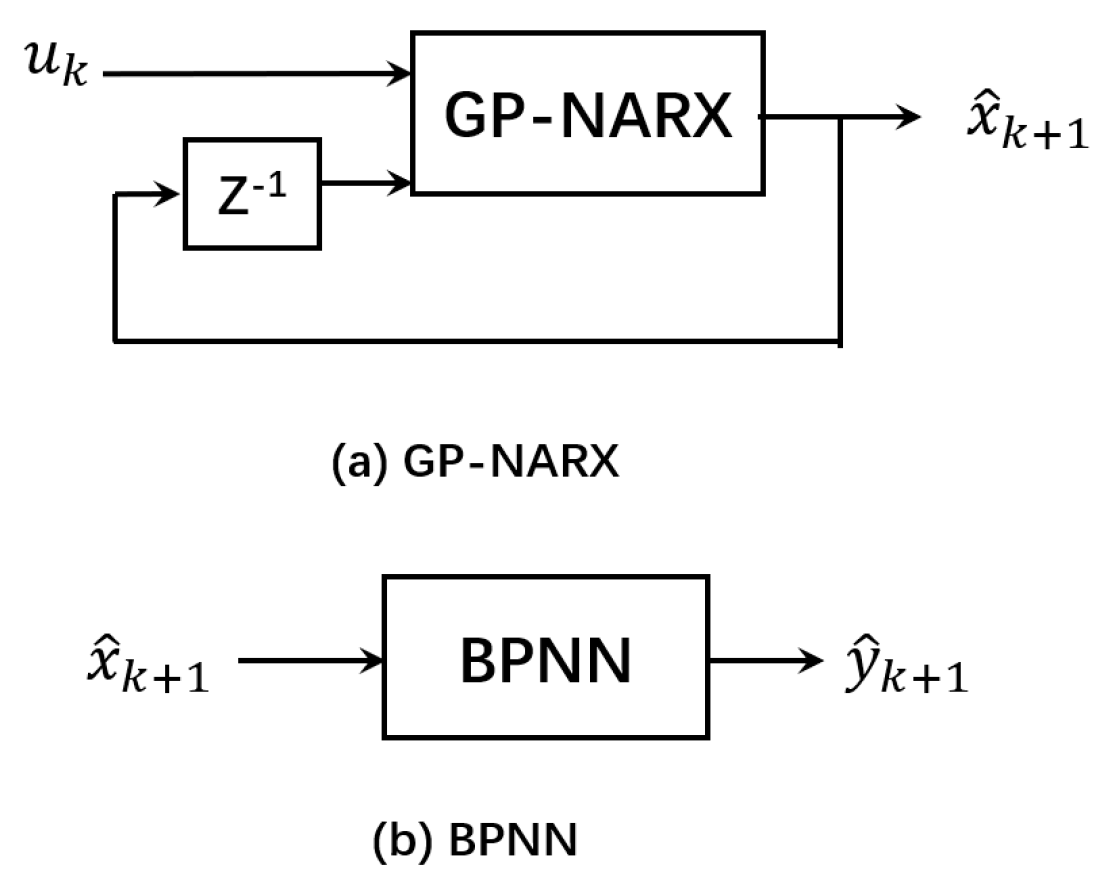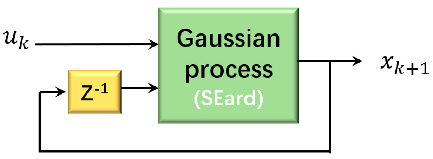The interactive force $y_k$ is the measurement model output, and joint vector $x_k$ whose elements include the joint angle and the angular velocity is treated as the state vector. Specifically, the GP-NARX with one-step time-delay feedback defined as $f(·)$ is applied in the state model, and the BPNN defined as $h(·)$ is applied as the measurement model in (26). The state space model framework is shown in Figure 3.

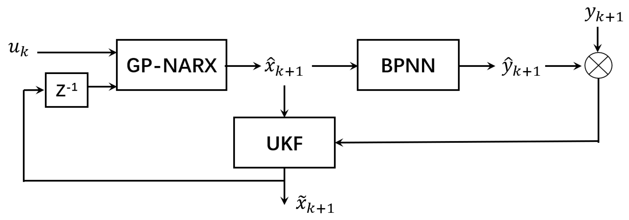
The state space model defined in (26) is first trained offline by a set of data, including the sEMG, joint angle, angular velocity and interactive force. Then, based on the trained GP-NARX and BPNN, the UKF algorithm is utilized to estimate the joint angle from sEMG signals and interactive force through the proposed SSM, as illustrated in Figure 4. The closed-loop nature of UKF makes the prediction more accurate. Then, the trained model is used for joint angle prediction.

4. Experimental Study and Discussion

4.1. Experimental Setup and Data Processing

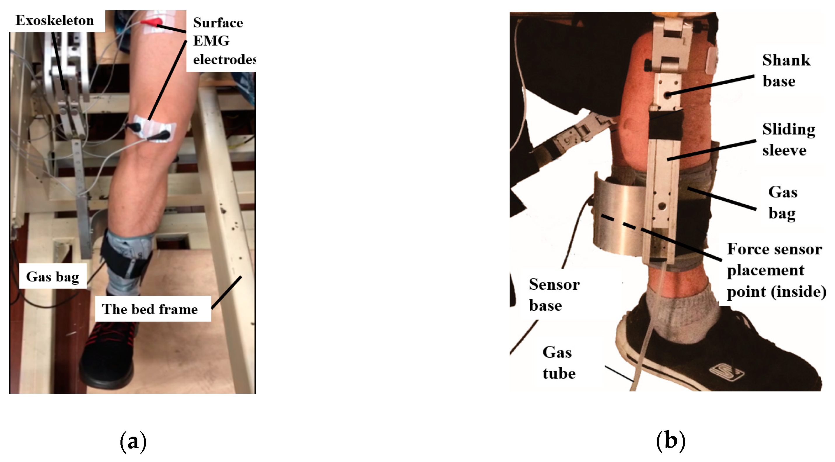
Experiments were conducted on the self-developed lower limb exoskeleton [46], as illustrated in Figure 5a. The applied robot was the combination of an exoskeleton robot and a bed which can turn from horizontal to 50°. As shown in Figure 5b, the shank part of the exoskeleton is composed of a shank base and a sliding sleeve. This mechanical structure is adopted so that the contact point between the user and the exoskeleton can be adjusted according to personal requirements before experiments. Once decided, the position will be fixed during the running process when the change of contact point in the process may give rise to reduced prediction performance. A force sensor is planted at the contact point and a gas bag is used to ensure the degree of comfort of the subject.

Six healthy men aged from 23 to 30 participated in the experiments. This work was approved by the Ethics Committee of Shanghai Jiao Tong University. All the subjects gave written informed consent prior to the participation in the study. Each subject was required to make voluntary and random knee flexions and extensions to drive the exoskeleton when the subject’s thigh was kept in parallel with the ground and the position of the knee joint was fixed. About seven sessions, in each of which the subject randomly flexed and extended his leg for about 40 s, were conducted for each participant. Every two sessions were separated by a rest of 3 min to avoid muscle fatigue. More sessions would be added when poor data collection quality or obvious errors could be observed and the corresponding results were excluded from the final analysis. The data of the first four sessions of random movements were used for training the motion prediction models, and the remaining three sessions were used as the test data for performance evaluation. During the whole process, the exoskeleton worked under the interactive force sensing and control mode. In this mode, the exoskeleton was driven by the motors to follow human motion in real-time. Through detecting the interactive force between the human and exoskeleton, the trajectory prediction and compensation were implemented. The detailed force control strategy can be found in [47].

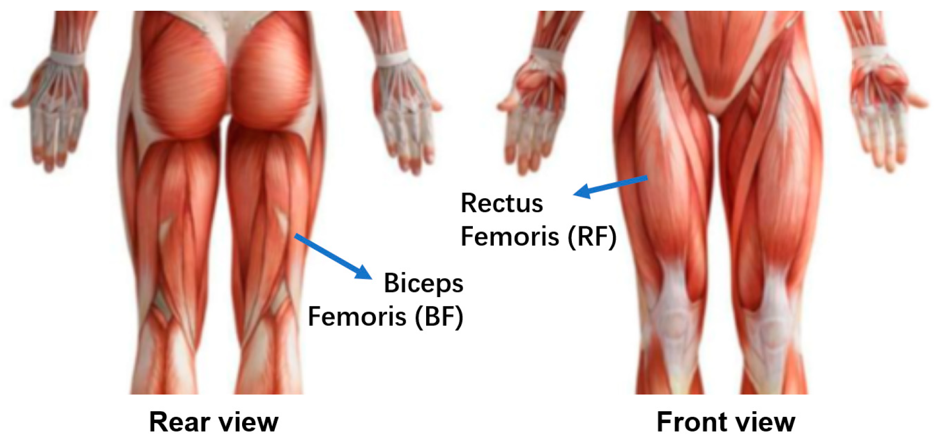
Disposable bi-polar Ag-AgCl surface EMG electrodes were used to collect the EMG signals from the RF. In our experiments, only the EMG signals from RF instead of those from both RF and BF were used to feature the muscle activation. The corresponding muscles are illustrated in Figure 6. There were two main reasons that the EMG signals from BF were not included in our model. The first was that the activation of BF stayed low and did not change much during the experiment process when the subject’s thigh was kept parallel to the ground [46]. This meant that the BF contributed little to the joint variation. The second reason is that reducing the number of inputs would largely increase the computational efficiency, especially when GP was included in our model [16,17].

The force signal was processed by a 3rd-order digital Butterworth filter of 0.01-1 Hz. The EMG signals were processed under the sampling frequency of 2000 Hz. A 4th-order digital Butterworth filter of 10-500 Hz and a notch-rectifier of 50 Hz (to remove the power noise) were applied to the EMG signals. The robust and stable energy kernel method was applied to process the EMG signals and extract the muscle activation when it integrated both the merits of RMS and MPF and reflected muscle recruitment level and firing rate at the same time [42]. The extracted feature of EMG signals was indicated as EK in the following. As only the EMG signal from RF was included, the dimension of the feature vector was 1.

4.2. Model Learning and Input Choice

Motion models were trained for each subject. The GP-NARX model was first trained using $u_k$ as the inputs and $x_k$ as the output. The model structure is illustrated in Figure 7. SE was chosen as the kernel function when the stationary nature and the smoothness assumption of this radial basis function regression model coincide with the joint angle variation. Specifically, the automatic relevance determination squared exponential (SEard) kernel was used to provide different hyperparameters for the three different inputs, including the extracted feature of EMG, the joint angle and the angular velocity. The model hyperparameters were optimized through minimizing the differentiable multivariate function using the conjugate gradients.

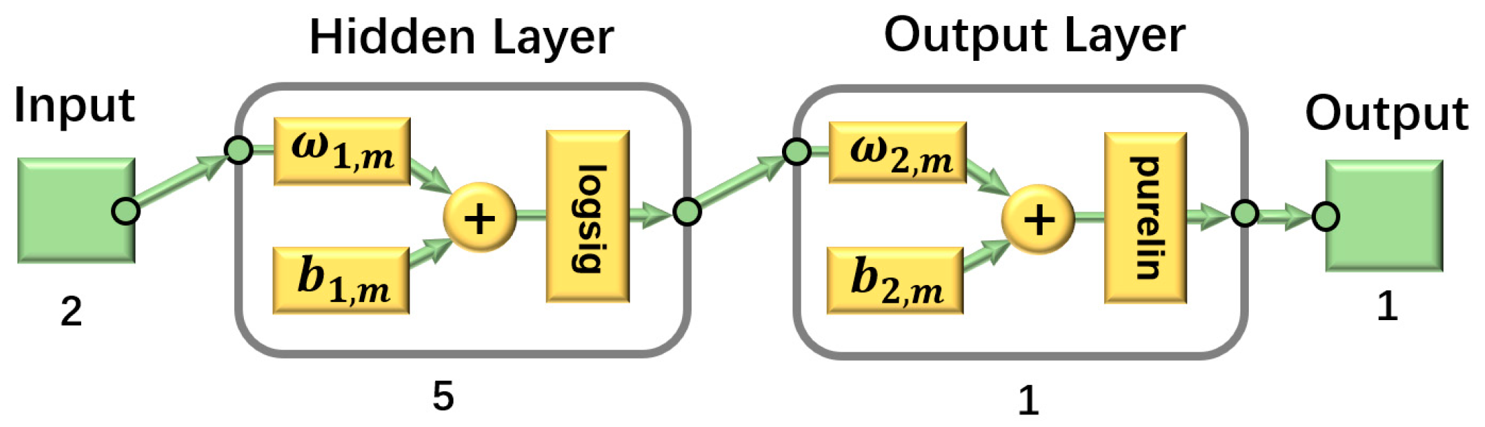
The BPNN included three layers (i.e., one input layer, one hidden layer, and one output layer). The input to the BPNN in the measurement model was the joint vector $x_k$ including the joint angle and angular velocity, and the interactive force $y_k$ was the model output. Thus, the dimension of the input vector was 2 and that of the output vector was 1. Sigmoid function (logsig) and linear function (purelin) were selected as the transfer functions of hidden and output layers, respectively, as illustrated in Figure 8. In order to decide the numbers of hidden layers and neurons, the correlation coefficient was used to evaluate the network performance. After many attempts, the number of hidden layers was chosen as 1 and the number of hidden neurons was chosen as 5 to achieve a tradeoff between computational efficiency and accuracy. The Levenberg-Marquardt method was used to optimize the net.

In fact, the joint angle instead of the joint vector containing both the joint angle and the angular velocity was also tested as the input to the measurement model. However, the performance was far from satisfactory even when more hidden layers and hidden neurons were used. It proved, from one aspect, that the biomechanical interpretation of human-exoskeleton interaction did provide a good foundation for the development of the measurement model. With the trained GP-NARX model and BPNN, the state space model formulated in (26) can be obtained and developed using the UKF algorithm.

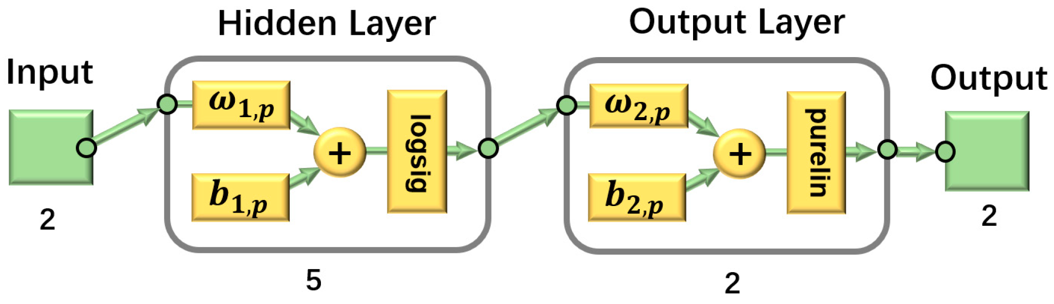
The way in which system models learn the mapping relations from neural signals to human joint angle varies, but ANN is one of the most widely used approaches [1]. Thus, different from the BPNN for the measurement model of SSM, a traditional BPNN, which used the extracted EMG features and the interactive force as the inputs and the joint vector containing the joint angle and angular velocity as the output, was also built for performance comparison. In consequence, the dimensions of the input vector and output vector were both 2. It was also found through numerous attempts that the increase of the numbers of hidden neurons and hidden layers did not improve the performance much. Thus, one hidden layer with 5 hidden neurons was also adopted here. Its architecture is illustrated in Figure 9.

4.3. Experimental Resuls

To better evaluate the performance of the proposed SSM, different evaluation criteria including the correlation coefficient (CC), root mean square error (RMSE), and the goodness of fit in terms of normalized mean square error (NMSE) are utilized. The goodness of fit in terms of NMSE is abbreviated as FIT in the following.

The Pearson CC of predicted values $\widehat{x}$ and actual values $x$ in terms of the covariance of $\widehat{x}$ and $x$ is defined as:

$$cc\left(\widehat{x},x_k\right)=\frac{cov\left(\widehat{x},x\right)}{{\sigma }_{\widehat{x}}{\sigma }_x}$$

(27)

where ${\sigma }_{\widehat{x}}$ and ${\sigma }_x$ are the standard deviation of $\widehat{x}$ and $x$, respectively.

The RMSE of predicted values $\widehat{x}$ with actual values $x$ for $T$ different predictions is given by:

$$RMSE=\sqrt{\frac{1}{T}{{\displaystyle \sum }}_1^T{\left({\widehat{x}}_k-x_k\right)}^2}$$

(28)

The cost function of the goodness of fit is chosen as NMSE in our application:

$$FIT=1-\frac{\Vert x-\widehat{x}{\Vert }^2}{\Vert x-mean{\left(x\right)}^2\Vert }$$

(29)

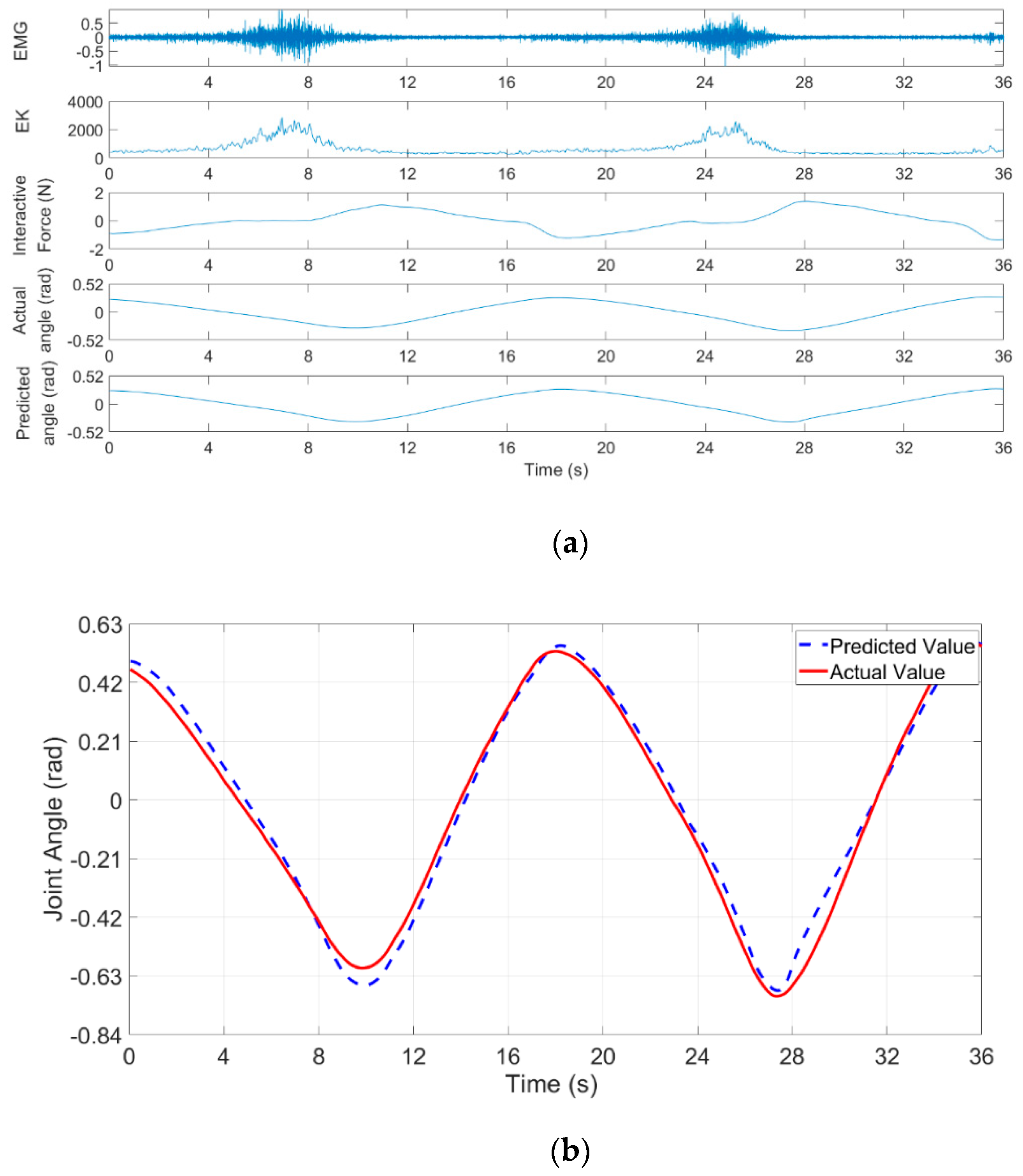
One typical segment of experimental results of Subject 1 (abbreviated as S1) using the proposed SSM is illustrated in Figure 10.

Referring to Figure 10a, the muscle activation could be well represented by the extracted EMG feature acquired from the energy kernel method. In addition, clear mapping relations could be observed between the interactive force and the joint angle. It also proved the rationality and necessity to include interactive force in the proposed model for the improvement of joint prediction performance.

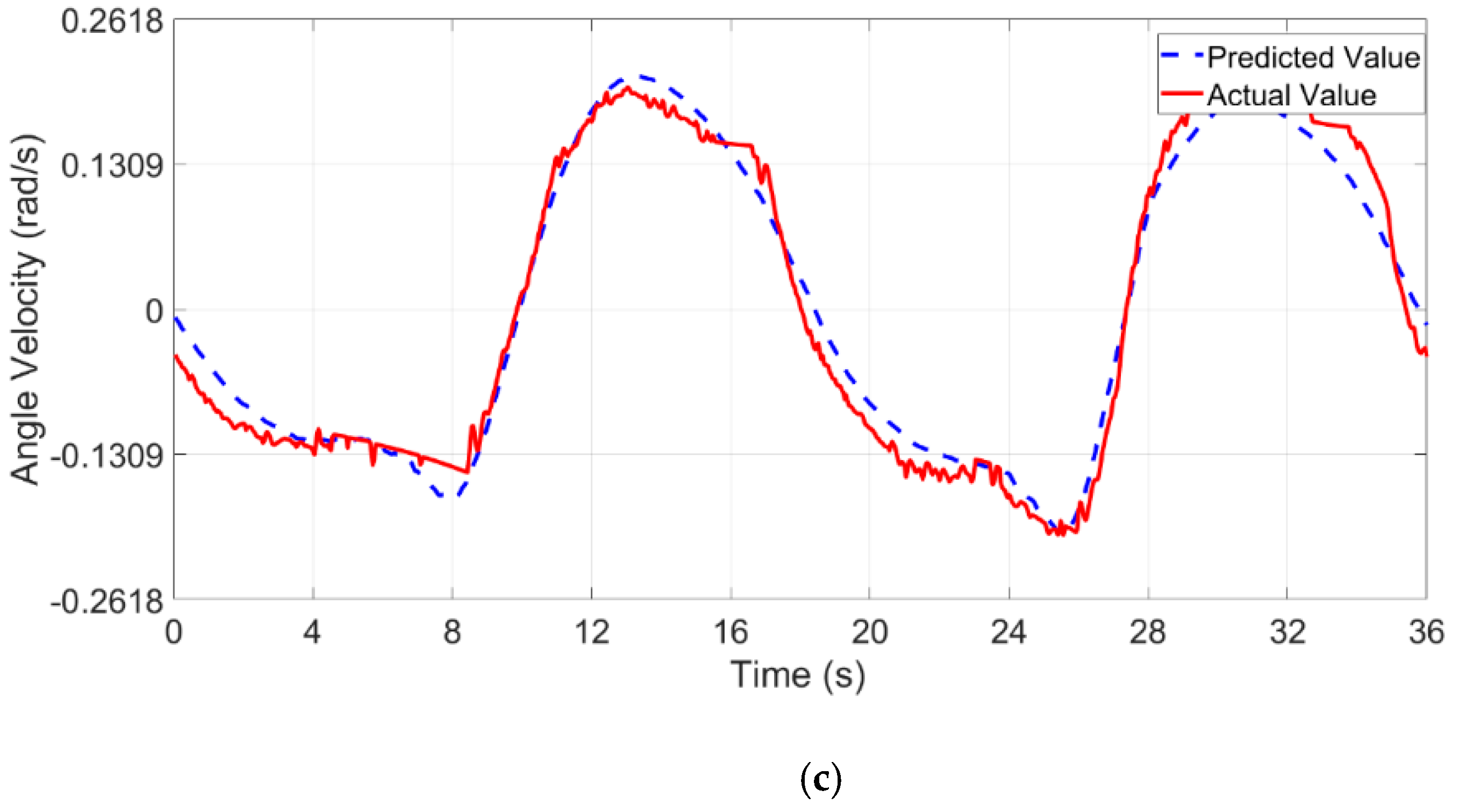
The joint angle and angular velocity prediction performance comparisons between the SSM and their actual values are illustrated in Figure 10b,c. A Wilcoxon signed rank test was used to calculate the corresponding p-value. As can be seen, although there existed local biases, the predicted values of both the angle and angular velocity could approximate their actual values well. Judging from different evaluation criteria, the SSM performances of the angle prediction were as follows: the CC was 0.9944, the RMSE was 0.0433 and the FIT was 0.9881 ($p<1\times {10}^{-3}$). The SSM prediction performances of the angular velocity were as follows: the CC was 0.9890, the RMSE was 0.0215 and the FIT was 0.9750 ($p=0.0034$). It could be found that the prediction performances were satisfactory, which reflected the feasibility and effectiveness of the proposed method.

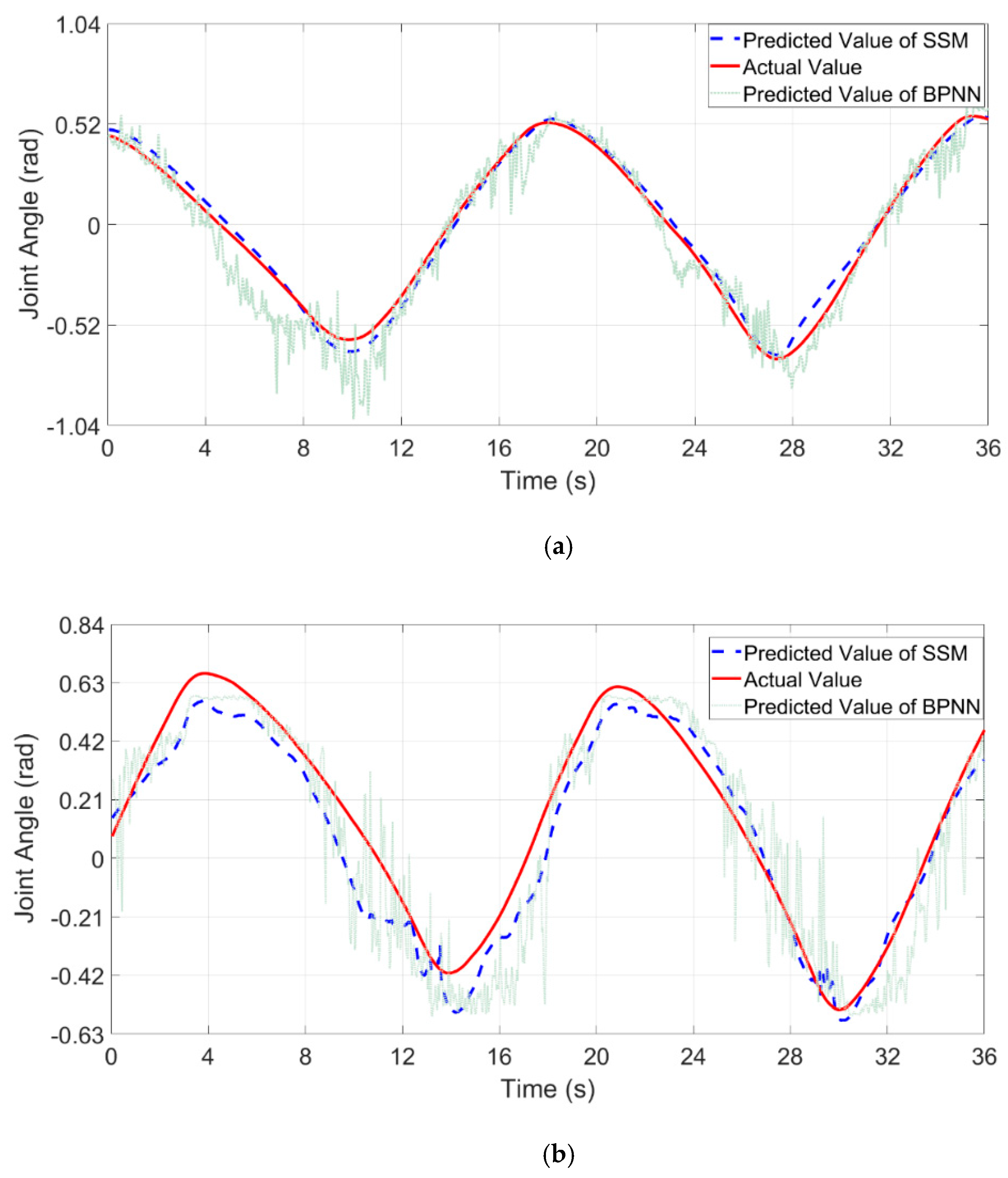
The same group of data from S1 was also processed with the traditional BPNN whose structure is illustrated in Figure 9. The joint prediction performance comparison is shown in Figure 11a. It could be found that the angle prediction of BPNN could still approximate the actual joint angle. However, compared with the results acquired from the proposed SSM, performances acquired from BPNN were worse when the CC was 0.9727 (decreased by 2.18%), the FIT was 0.9264 (decreased by 6.24%), and the RMSE increased to 0.1077 from 0.0433 ($p<1\times {10}^{-5}$). Although the overall prediction trend of BPNN was consistent with the actual angle variation when both the FIT and CC were acceptable, visible fluctuations could not be overlooked in Figure 11a. The reason that led to the fluctuations may be the nonstationarity of the EMG signal when it was one of the inputs to the model, and different from the proposed SSM, the BPNN was not able to make the EMG signal sufficiently smoothed. Such fluctuations might be fatal to the potential applications in the prediction control of exoskeleton systems when the position prediction error would give rise to huge interactive forces between human and exoskeleton. These extra loads would not only bring about extra burdens to the users, but may also lead to secondary damage when used in rehabilitation applications. The fluctuations in the BPNN prediction results also demonstrated the superiority of the proposed SSM over traditional BPNN when no visible fluctuation could be found in the SSM prediction results.

The joint prediction performance comparison between SSM and BPNN of S2 is illustrated in Figure 11b. Although the SSM performance of S2 was worse than that of S1 when bigger derivations could be observed, the results were still acceptable when the FIT was 0.9309, the CC was 0.9759, and the RMSE was 0.0941 ($p<1\times {10}^{-5}$). In addition, it could be found that performance of S2 using SSM was also better than that using BPNN. Compared to SSM, the corresponding values of BPNN were as follows: the FIT was 0. 8229 (decreased by 11.61%), the CC was 0.9372 (decreased by 3.97%), and the RMSE increased to 0.1525 from 0.0941 ($p<1\times {10}^{-5}$). Same as the results of S1 displayed in Figure 11a, there were visible fluctuations which seemed to be even more intense. That would be unacceptable when applied in human-exoskeleton systems.

Although not illustrated in the figure, the angular velocity prediction performances of S2 using the proposed SSM were also satisfactory when the corresponding CC was 0.9879, the FIT was 0.9687 and the RMSE was 0.0252 ($p<1\times {10}^{-5}$). Compared to SSM, the performances of BPNN were worse when the CC was 0.8751 (decreased by 11.42%), the FIT was 0.7415 (decreased by 23.46%) and the RMSE increased to 0.0738 from 0.0252 ($p<1\times {10}^{-5}$). These results also demonstrated the advantage of the proposed SSM over traditional BPNN in the angular velocity prediction. Given that our emphasis was put on the joint angle prediction, the angle velocity comparison was not further discussed.

In addition to the comparisons in Figure 11, the prediction performance comparisons of all the participated subjects including S3 to S6 were also conducted. The results of RMSE, CC and FIT were calculated using (27)–(29) and are displayed in

Table 1. Values of RMSE, CC and FIT of different models in terms of joint angle prediction for all the subjects.

		RMSE (rad)	CC	Fit
S1	SSM	$0.0513\pm 0.0079$	$0.9935\pm 0.0008$	$0.9852\pm 0.0029$
	BPNN	$0.1217\pm 0.0140$	$0.9681\pm 0.0046$	$0.9166\pm 0.0097$
S2	SSM	$0.1017\pm 0.0170$	$0.9817\pm 0.0049$	$0.9390\pm 0.0186$
	BPNN	$0.1982\pm 0.0379$	$0.9207\pm 0.0117$	$0.7962\pm 0.0316$
S3	SSM	$0.0588\pm 0.0167$	$0.9738\pm 0.0189$	$0.8891\pm 0.1019$
	BPNN	$0.1942\pm 0.0603$	$0.6699\pm 0.0720$	$0.3902\pm 0.0958$
S4	SSM	$0.0607\pm 0.0206$	$0.9704\pm 0.0182$	$0.9247\pm 0.0342$
	BPNN	$0.0938\pm 0.0572$	$0.9065\pm 0.0878$	$0.8232\pm 0.1502$
S5	SSM	$0.1093\pm 0.0261$	$0.9697\pm 0.0152$	$0.9292\pm 0.0312$
	BPNN	$0.2294\pm 0.0090$	$0.8516\pm 0.0149$	$0.7083\pm 0.0151$
S6	SSM	$0.1061\pm 0.0165$	$0.9751\pm 0.0045$	$0.9309\pm 0.0135$
	BPNN	$0.1961\pm 0.0283$	$0.8838\pm 0.0063$	$0.7672\pm 0.0172$

Note: S1, S2, …, S6 represent the six subjects; RMSE is the root mean square error, CC is the correlation coefficient, Fit is the goodness of fit in terms of NMSE; SSM is the state space model, BPNN is the back propagation neural network.

. It could be clearly observed that obvious improvements were achieved through the application of the proposed SSM instead of BPNN when all the values of CC and FIT were increased and values of RMSE were decreased for the 6 participated subjects. Individual differences could also be observed. In addition to the nonstationarity of EMG signals as the input, the differences were probably caused by the fact that the acquired signal qualities from different subjects differed greatly. Especially for S3, the performances using BPNN were poor. Various attempts, including increasing the numbers of hidden layers and neurons in each layer, have been made to improve the performance and acquire the best-fit network. However, the prediction results using BPNN were still unacceptable. The reasons behind still needed further investigations. In contrary, the corresponding SSM performances were much more acceptable, which demonstrated the robustness of the proposed SSM. Except for S3, the BPNN performances of other participated subjects were all acceptable. When we ignore the results of S3, the improvements when applying the proposed SSM instead of BPNN were achieved regardless of individual differences. The results demonstrated the advantages of the proposed SSM over traditional BPNN when applied in joint angle prediction, and the effectiveness of the SSM was also proven.

4.4. Further Discussions

Another issue that has to be made clear is whether the loads on the knee joint have impacts on the effectiveness of the proposed model. There are always loads on the knee joint during most of the cases, such as the situation when a standing position is adopted. Considering that the applied exoskeleton robot was the combination of a bed and an exoskeleton robot, there would be loads on the knee joint when there was an angle between the bed and the ground during the experiments. Although the bed could not turn to the vertical position because of safety considerations and equipment restrictions, the load impacts on the proposed model could be verified.

Thus, to demonstrate that the method did work, not only in the sitting down position, but was also suitable for other applications, the upper part of the bed was risen to about 30 degrees to the ground to find out the load impacts on the effectiveness of the proposed model. A small angle was adopted for safety considerations. Additional experiments were conducted. The resulting CC values were all above 0.95, which were similar to the main parts of the experiments when the sitting down position was adopted. The satisfactory results demonstrated that based on the inputs of extracted EMG features and interactive force, the proposed SSM model was able to predict the joint angle continuously when there were loads on the knee joint.

In fact, joint angle learning and prediction has long been a research hotspot. Instead of using GP-based models, traditional neural networks were usually applied [1]. For instance, Ding et al. developed a general state-space model, in which a traditional neural network-based NARX model was integrated with BPNN [4]. They have done a very good job in continuously and accurately estimating the multi-joint movements through the use of a nonlinear filtering algorithm. The CC values of the four predicted angles were 0.95, 0.96, 0.96 and 0.95, which were all close to 1. Compared with their work, we concentrated on the learning and prediction of one joint angle instead of four, and improved the performance, as illustrated in Table 1. It should be recognized that the decrease of the joint angle number needed to be predicted might be one reason for the improvements. There might also be other possible reasons that contributed to the improvements. One reason was that the addition of interactive force in our model would improve the performance of joint angle prediction [30]. The use of nonredundant and redundant sub-vectors of EMG signals were innovative in their study, but the information acquired only from the EMG signals was still limited. The other reason might be the use of GP when the integration of parametric model and non-parametric model of GP would improve the performance [48]. In addition, they also made the comparison between the state space model and the use of NARX model alone. A conclusion was reached that the estimation using the integration of NARX and BPNN over the prediction with the NARX model alone had two improvements: (1) the estimation was closer to the “true” angles, and the larger errors have been corrected by the measurement equation; (2) the UKF made the estimation smoother, which would be beneficial for the stable control of the robots. The second conclusion could also be used to explain the differences observed in our experimental results shown in Figure 11 when the fluctuations were only found using BPNN instead of the proposed SSM integrating GP-NARX with BPNN.

To take the advantages of GP-based models, Michele et al. also used a GP-NARX model that combined the context of pervious hand movement with instantaneous muscle activity to predict future hand movements [23]. In addition to EMG signals, mechanomyographic (MMG) signals were also used to indicate hand muscle activation in the forearm. Referring to their results, the improvement of fusing MMG with EMG in the GP-NARX model was relatively small. Thus, it was reasonable to only include EMG in the angle prediction model when taking the computational cost into consideration. GP was also used to estimate the ankle angle and torque based on shank angular velocity and angle without information from neural signals [16]. In their study, they showed that it was not necessary to acquire speed determination, gait percent identification, lookup tables, or switching rules to continuously mapping the input to the output.

However, all the above studies treated the whole neural control process of human movement as a black-box problem without providing any biomechanical interpretations. In contrast, there are also studies which used Hill’s muscle model to develop the forward dynamics of human neuromusculoskeletal system for angle prediction [27]. Similar to all the model-based methods, parameter identification, which is very time-consuming, must be done in advance. Thus, the proposed method which is a trade-off between engineering application using machine learning techniques and theoretical analysis providing the biomechanical interpretations might be the optimal choice.

As stated, one major difference of our method is to bring GP into the state space model. When GP is generally considered equivalent in terms of performance to conventional artificial neural network approaches, it is in fact formally equivalent to a neural network with an infinite number of units in the hidden layer [49]. However, these unique benefits of GP over a standard neural network come at a cost. GP regression is numerically complex and the heavy computational cost is always its major drawback. This leads to the fact that the computational efficiency of the current method seriously limits its adoption in real-time applications. To overcome this limitation, numerous researchers have suggested different sparse approximations, including the subset of data (SoD) approximation, fully independent training conditional (FITC) approximation, and partially independent training conditional (PITC) approximation. One successful application in joint angle prediction can be found in [44] where an online sparse GP algorithm is proposed to learn the human motion intent. In addition, the integration with an evolving system would be another choice [22]. Also, constant advances in embedded processing have resulted in GP being successfully deployed in real-time activity recognition in smartphone-based settings using state-of-the-art low-power embedded processors [50,51]. How to integrate these techniques into the proposed method and increase the computation efficiency to meet the real-time requirements in the prediction control of exoskeleton system would be the focus of our future research.

5. Conclusions

This paper develops a state space model for continuous joint angle prediction in a human-exoskeleton system. In addition to the EMG signals, interactive force is also applied as the input to the proposed model. Hill’s muscle model and SP muscular model are adopted to feature the biomechanical interpretations for the forward dynamics of the knee joint and the interactive force generation. In consequence, the impact of interactive force on the human-exoskeleton system is also considered. Based on the intrinsic connections among the variables, including the EMG signals, the interactive force and the corresponding joint angle, the state model and measurement model of the SSM are developed. The GP-NARX model and BPNN are integrated to combine the relative strengths of both the non-parametric model and parametric model. They are utilized to bypass the problem of parameter identification and provide better adaptivity and feasibility for the model in practical engineering. Corresponding experimental results demonstrate the validity and superiority of the method. Judging from different evaluation criteria, including the CC, the FIT and the RMSE, obvious improvements were achieved through the application of the proposed SSM over traditional BPNN when the values of CC and FIT were increased and those of RMSE were decreased for all 6 subjects. Load impacts on the effectiveness of the method were also discussed. Future research should improve the computational efficiency of the proposed method so that it could be better applied in the prediction control of human-exoskeleton systems.

References

1. Losey, D.P.; McDonald, C.G.; Battaglia, E.; O’Malley, M.K. A Review of Intent Detection, Arbitration, and Communication Aspects of Shared Control for Physical Human–Robot Interaction. Appl. Mech. Rev. 2018, 70, 010804. [Google Scholar] [CrossRef]
2. Goodrich, M.A.; Schultz, A.C. Human-Robot Interaction: A Survey. Found. Trends Hum. Comput. Interact. 2007, 1, 203–275. [Google Scholar] [CrossRef] [Green Version]
3. Erden, M.S.; Tomiyama, T. Human-Intent Detection and Physically Interactive Control of a Robot without Force Sensors. IEEE Trans. Robot. 2010, 26, 370–382. [Google Scholar] [CrossRef]
4. Ding, Q.; Han, J.; Zhao, X. Continuous estimation of human multi-joint angles from sEMG using a state-space model. IEEE Trans. Neural Syst. Rehabil. Eng. 2017, 25, 1518–1528. [Google Scholar] [CrossRef] [PubMed]
5. Zajac, F.E. Muscle and tendon Properties models scaling and application to biomechanics and motor. Crit. Rev. Biomed. Eng. 1989, 17, 359–411. [Google Scholar] [PubMed]
6. Zahalak, G.I. A Comparison of the Mechanical Behavior of the Cat Soleus Muscle with a Distribution-Moment Model. J. Biomech. Eng. 1986, 108, 131. [Google Scholar] [CrossRef] [PubMed]
7. Zahalak, G.I. The Two-state Cross-bridge Model of Muscle is an Asymptotic Limit of Multi-state Models. J. Theor. Biol. 2000, 204, 67–82. [Google Scholar] [CrossRef]
8. Hill, A.V. The heat of shortening and the dynamic constants of muscle. Proc. R. Soc. Lond. Ser. B 1938, 126, 136–195. [Google Scholar] [Green Version]
9. Huxley, A.F.; Simmons, R.M. Proposed mechanism of force generation in striated muscle. Nature 1971, 233, 533–538. [Google Scholar] [CrossRef]
10. Buchanan, T.S.; Lloyd, D.G.; Manal, K.; Besier, T.F. Neuromusculoskeletal modeling: Estimation of muscle forces and joint moments and movements from measurements of neural command. J. Appl. Biomech. 2004, 20, 367–395. [Google Scholar] [CrossRef]
11. Bogey, R.A.; Barnes, L.A. An EMG-to-Force Processing approach for estimating in vivo hip muscle forces in normal human walking. IEEE Trans. Neural Syst. Rehabil. Eng. 2017, 25, 1172–1179. [Google Scholar] [CrossRef]
12. Falisse, A.; Rossom, S.V.; Jonkers, I.; De Groote, F. EMG-driven optimal estimation of subject-specific Hill model muscle-tendon parameters of the knee joint actuators. IEEE Trans. Biomed. Eng. 2017, 64, 2253–2262. [Google Scholar] [PubMed]
13. Sartori, M.; Reggiani, M.; Farina, D.; Lloyd, D.G. EMG-driven forward-dynamic estimation of muscle force and joint moment about multiple degrees of freedom in the human lower extremity. PLoS ONE 2012, 7, e52618. [Google Scholar] [CrossRef] [PubMed]
14. Tran, H.T.; Cheng, H.; Lin, X.C.; Duong, M.-K.; Huang, R. The relationship between physical human-exoskeleton interaction and dynamic factors: Using a learning approach for control applications. Sci. China Inf. Sci. 2014, 57, 1–13. [Google Scholar] [CrossRef]
15. Hamaya, M.; Matsubara, T.; Noda, T.; Morimoto, J. Learning assistive strategies for exoskeleton robots from user-robot physical interaction. Pattern Recogn. Lett. 2017, 99, 67–76. [Google Scholar] [CrossRef]
16. Eslamy, M.; Alipour, K. Synergy-Based Gaussian Process Estimation of Ankle Angle and Torque: Conceptualization for High Level Controlling of Active Robotic Foot Prostheses/Orthoses. J. Biomech. Eng. 2019, 141, 021002. [Google Scholar] [CrossRef]
17. Rasmussen, C.E.; Williams, C.K.I. Gaussian Processes for Machine Learning; MIT Press: Cambridge, MA, USA, 2006. [Google Scholar]
18. Roberts, S.; Osborne, M.; Ebden, M.; Reece, S.; Gibson, N.; Aigrain, S. Gaussian processes for time-series modelling. Philos. Trans. Soc. A: Math. Phys. Eng. Sci. 2012, 371, 20110550. [Google Scholar] [CrossRef] [PubMed]
19. Michieletto, S.; Tonin, L.; Antonello, M.; Bortoletto, R.; Spolaor, F.; Pagello, E.; Menegatti, E. GMM-Based Single-Joint Angle Estimation Using EMG Signals. Intelligent Autonomous Systems 13; Springer: Cham, Switzerland, 2016; pp. 1173–1184. [Google Scholar]
20. Belić, J.J.; Aldo Faisal, A. Decoding of human hand actions to handle missing limbs in neuroprosthetics. Front. Comput. Neurosci. 2015, 9, 27. [Google Scholar] [CrossRef] [PubMed]
21. Chen, X.; Zeng, Y.; Yin, Y. Improving the transparency of an exoskeleton knee joint based on the understanding of motor intent using energy kernel method of EMG. IEEE Trans. Neural Syst. Rehabil. Eng. 2017, 25, 577–588. [Google Scholar] [CrossRef] [PubMed]
22. Zeng, Y.; Yang, J.T.; Peng, C.; Yin, Y. Evolving Gaussian Process Autoregression based Learning of Human Motion Intent Using Improved Energy Kernel Method of EMG. IEEE Trans. Biomed. Eng. 2019. [Google Scholar] [CrossRef]
23. Xiloyannis, M.; Gavriel, C.; Thomik, A.A.C.; Faisal, A.A. Gaussian process autoregression for simultaneous proportional multi-modal prosthetic control with natural hand kinematics. IEEE Trans. Neural Syst. Rehabil. Eng. 2017, 25, 1785–1801. [Google Scholar] [CrossRef]
24. Chen, J.; Zhang, X.; Cheng, Y.; Xi, N. Surface EMG based continuous estimation of human lower limb joint angles by using deep belief networks. Biomed. Signal Process. Control 2018, 40, 335–342. [Google Scholar] [CrossRef]
25. Winby, C.R.; Lloyd, D.G.; Besier, T.F.; Kirk, T.B. Muscle and external load contribution to knee joint contact loads during normal gait. J. Biomech. 2009, 42, 2294–2300. [Google Scholar] [CrossRef]
26. Ao, D.; Song, R.; Gao, J.W. Movement Performance of Human-Robot Cooperation Control Based on EMG-driven Hill-type and Proportional Models for an Ankle Power-assist Exoskeleton Robot. IEEE Trans. Neural Syst. Rehabil. Eng. 2017, 25, 1125–1134. [Google Scholar] [CrossRef]
27. Han, J.; Ding, Q.; Xiong, A.; Zhao, X. A state-space EMG model for the estimation of continuous joint movements. IEEE Trans. Ind. Electron. 2015, 62, 4267–4275. [Google Scholar] [CrossRef]
28. Wakita, K.; Huang, J.; Di, P.; Sekiyama, K.; Fukuda, T. Human-Walking-Intention-Based Motion Control of an Omnidirectional-Type Cane Robot. IEEE/ASME Trans. Mechatron. 2013, 18, 285–296. [Google Scholar] [CrossRef]
29. Pehlivan, A.U.; Losey, D.P.; Ormalley, M.K. Minimal Assist-as-Needed (mAAN) Controller for Upper Limb Robotic Rehabilitation. IEEE Trans. Robot. 2015, 32, 113–124. [Google Scholar] [CrossRef]
30. Tang, Z.; Yu, H.; Cang, S. Impact of load variation on joint angle estimation from surface EMG signals. IEEE Trans. Neural Syst. Rehabil. Eng. 2016, 24, 1342–1350. [Google Scholar] [CrossRef] [PubMed]
31. Chen, X.; Yin, Y.H. A highly efficient semiphenomenological model of a half-sarcomere for real-time prediction of mechanical behavior. J. Biomech. Eng. 2014, 136, 121001. [Google Scholar] [CrossRef]
32. Lloyd, D.G.; Besier, T.F. An EMG-driven musculoskeletal model to estimate muscle forces and knee joint moments in vivo. J. Biomech. 2003, 36, 765–776. [Google Scholar] [CrossRef] [Green Version]
33. Fleischer, C.; Hommel, G. A human--exoskeleton interface utilizing electromyography. IEEE Trans. Robot. 2008, 24, 872–882. [Google Scholar] [CrossRef]
34. Karavas, N.; Ajoudani, A.; Tsagarakis, N.; Saglia, J.; Bicchi, A.; Caldwell, D. Tele-impedance based assistive control for a compliant knee exoskeleton. Robot. Auton. Syst. 2015, 73, 78–90. [Google Scholar] [CrossRef]
35. Dorgan, S.J.; O’Malley, M.J. A mathematical model for skeletal muscle activated by N-let pulse trains. IEEE Trans. Rehabil. Eng. 1998, 6, 286–299. [Google Scholar] [CrossRef] [PubMed]
36. Kellermayer, M.S.Z.; Smith, S.B.; Granzier, H.L.; Bustamante, C. Folding-unfolding transitions in single titin molecules characterized with laser tweezers. Science 1997, 276, 1112–1116. [Google Scholar] [CrossRef] [PubMed]
37. Ramírez, A.; Grasa, J.; Alonso, A.; Soteras, F.; Osta, R.; Muñoz, M.; Calvo, B. Active response of skeletal muscle: In vivo experimental results and model formulation. J. Theor. Biol. 2010, 267, 546–553. [Google Scholar] [CrossRef] [PubMed]
38. Gordon, A.M.; Huxley, A.F.; Julian, F.J. The variation in isometric tension with sarcomere length in vertebrate muscle fibres. J. Physiol. 1966, 184, 170–192. [Google Scholar] [CrossRef] [PubMed] [Green Version]
39. Heckathorne, C.W.; Childress, D.S. Relationship of the surface electromyogram to the force, length, velocity, and contraction rate of the cineplastic arm. Am. J. Phys. Med. 1981, 60, 1–19. [Google Scholar] [PubMed]
40. Zuniga, E.N.; Simons, D.G. Nonlinear relationship between electromyographam potential and muscle tension in normal subjects. Arch. Phys. Med. Rehabil. 1969, 50, 613–620. [Google Scholar]
41. Woods, J.J.; Bigland-Ritchie, B. Linear and non-linear surface EMG/force relationships in human muscles. An anatomical/functional argument for the existence of both. Am. J. Phys. Med. 1983, 62, 287–299. [Google Scholar]
42. Chen, X.; Yin, Y.; Fan, Y. EMG oscillator model-based energy kernel method for characterizing muscle intrinsic property under isometric contraction. Chin. Sci. Bull. 2014, 59, 1556–1567. [Google Scholar] [CrossRef]
43. Denoth, J.; Stüssi, E.; Csucs, G.; Danuser, G. Single Muscle Fiber Contraction Is Dictated by Inter-Sarcomere Dynamics. J. Theor. Biol. 2002, 216, 101–122. [Google Scholar] [CrossRef] [PubMed]
44. Long, Y.; Du, Z.-J.; Wang, W.-D.; Dong, W. Human motion intent learning based motion assistance control for a wearable exoskeleton. Robot. Comput. Integr. Manuf. 2018, 49, 317–327. [Google Scholar] [CrossRef]
45. Julier, S.J.; Uhlmann, J.K. New extension of the Kalman filter to nonlinear systems. Proc. SPIE 1997, 3068, 182–194. [Google Scholar]
46. Fan, Y.; Yin, Y. Active and progressive exoskeleton rehabilitation using multisource information fusion from EMG and force-position EPP. IEEE Trans. Biomed. Eng. 2013, 60, 3314–3321. [Google Scholar] [CrossRef]
47. Yin, Y.H.; Xu, Y.; Jiang, Z.H.; Wang, Q.R. Tracking and understanding unknown surface with high speed by force sensing and control for robot. IEEE Sens. J. 2012, 12, 2910–2916. [Google Scholar] [CrossRef]
48. Fernandez, R.; Rendel, A.; Ramabhadran, B.; Hoory, R. F0 contour prediction with a deep belief network-Gaussian process hybrid model. In Proceedings of the 2013 IEEE International Conference on Acoustics, Speech and Signal Processing, Vancouver, BC, Canada, 26–31 May 2013; pp. 6885–6889. [Google Scholar]
49. MacKay, D.J.C. Gaussian Processes-a Replacement for Supervised Neural Networks? Cavendish Laboratory, University of Cambridge: Cambridge, UK, 1997. [Google Scholar]
50. Zhang, L.; Liu, J.; Jiang, H.; Guan, Y. SensTrack: Energy-efficient location tracking with smartphone sensors. IEEE Sens. J. 2013, 13, 3775–3784. [Google Scholar] [CrossRef]
51. Shin, H.; Chon, Y.; Cha, H. Unsupervised construction of an indoor floor plan using a smartphone. IEEE Trans. Syst. Man Cybern. Part C (Appl. Rev.) 2012, 42, 889–898. [Google Scholar] [CrossRef]
Figure 1. Representation of the muscle–tendon unit based on Hill’s muscle model. The muscle–tendon unit is modeled as a muscle fiber in series with a tendon. Structures putatively responsible for the muscle force are called the passive element (PE) and the contractile element (CE).
Applsci 09 01711 g001
Figure 2. Mechanical approximation of the human knee joint and the rotational motion of human-machine synthetic model.
Applsci 09 01711 g002
Figure 3. The state space model framework, where GP-NARX and BPNN are utilized in the state model and measurement model; x ^ k + 1 and y ^ k + 1 are the predicted values of x k + 1 and y k + 1
Applsci 09 01711 g003
Figure 4. Joint angle prediction from the muscle activation and interactive force where x ˜ k + 1 represents the estimated value of x k + 1 calculated by the UKF
Applsci 09 01711 g004
Figure 5. Experimental setup. (a) The self-developed lower-limb exoskeleton worn by the experimental subject and the bed framework, (b) the shank part of the exoskeleton.
Applsci 09 01711 g005
Figure 6. Rear and front view of the human thigh illustrating the selected two muscles. In our application here, the electrodes were placed only on the RF.
Applsci 09 01711 g006
Figure 7. The GP-NARX model, where the extracted EMG feature u k is the input and the joint vector x k + 1 is the output
Applsci 09 01711 g007
Figure 8. The BPNN for the measurement model of SSM, where ω 1 , m and ω 2 , m are the weights, b 1 , m and b 2 , m are the bias values. The input vector x k whose dimension is 2 contains the joint angle and angular velocity, and the output vector y k whose dimension is 1 contains the interactive force, and 2, 5 and 1 are the numbers of the neurons.
Applsci 09 01711 g008
Figure 9. The BPNN for performance comparison with the SSM, where ω 1 , p and ω 2 , p are the weights, b 1 , p and b 2 , p are the bias values. Different from the BPNN for the measurement model of SSM, the input vector x k whose dimension is 2 contains the extracted EMG feature and the interactive force, and the output vector y k whose dimension is 2 contains the joint angle and angular velocity, and 2, 5 and 2 are the numbers of the neurons.
Applsci 09 01711 g009
Figure 10. A typical set of experimental results. (a) The raw EMG signals from RF, the extracted energy kernel feature (EK), the interactive force, the actual angle and the predicted angle are listed from top to bottom; (b) The results of predicted and actual joint angle; (c) The results of predicted and actual joint angular velocity.
Applsci 09 01711 g010aApplsci 09 01711 g010b
Figure 11. Joint prediction performance comparisons between the BPNN and SSM. (a) S1, (b) S2.
Applsci 09 01711 g011