Cyclic p-y Curves of Monopiles in Dense Dry Sand Using Centrifuge Model Tests

Abstract

In this study, centrifuge model tests were used to examine the lateral behavior of a monopile embedded in dry sand through cyclic lateral loading tests. The soil specimens used in the tests were dry Jumunjin sand with a relative density of 80% and a friction angle of 38°. A static loading test was performed once, and cyclic loading tests were performed four times using four magnitudes of cyclic load (30%, 50%, 80%, and 120% of static lateral capacity). The experimental cyclic p-y curve was obtained through the tests, and the maximum soil resistance points that were found for each load were used to find the cyclic p-y backbone curve for each depth. The two variables which are needed to define the cyclic p-y backbone curve, i.e., the initial modulus of subgrade reaction (k_ini) and ultimate soil resistance (p_u), were suggested as functions of the soil’s physical properties and the pile. The cyclic p-y curve of the first cycle and the 100th cycle were formulated to present the upper limit and lower limit. The suggested cyclic p-y curve had an overestimated soil resistance compared with the existing API (1987) method, but the initial modulus of subgrade reaction was underestimated.

1. Introduction

Many domestic and international studies have been performed on the behavior of piles exposed to vertical loads and considerable research has been actively conducted on the behavior of piles subjected to lateral loads. Piles that are exposed to lateral loads, due to actions such as wind, will experience greater moments than piles exposed to vertical loads. Because of this, it is necessary to study the behavior related to the lateral loading of piles. Achmus et al. [1] used numerical analysis and performed cyclic loading of a monopile in 102–104 cycles to study the long-term behavior of the soil. Møller and Christiansen [2] performed static and cyclic loading tests on monopiles on a small scale, and these were numerically analyzed and compared. Kim et al. [3] used a Strain Wedge Model (SWM) to perform 1–10⁵ cycles of lateral loading on a monopile, and they also studied the pile head displacement and initial stiffness, according to the increase in cycles. Peralta [4] performed one-way cyclic loading tests on a pile with a diameter of 60 mm in sand with a relative density of 40% and 60%. Various loads were used, and 10,000 load cycles were performed. Roesen et al. [5] performed cyclic loading tests using a pile with a diameter of 60 mm, loaded for 46,000 cycles at relative densities of 78% and 87%. Gerber and Rollins [6] performed cyclic loading tests on a steel pipe pile with a diameter of 324 mm in full scale to find the so-called p-y curve. The p-y curve is used to analyze the pile lateral support behavior. Here, p is the soil resistance, and y is the displacement. Fan and Long [7] examined the effect of changes in the pile diameter on the p-y curve and found that the effect was slight. The p-y curves which are commonly used now were presented by API [8] and calculated from experiment values obtained by Matlock [9] in clay and from static and cyclic experiments by Cox et al. [10] in sandy soil. In addition to this, there are other types of p-y curves, such as the Reese [11] p-y curve and the NCHRP [12] p-y curve. However, because these were formulated using results obtained from experiments on piles with diameters smaller than 1 m, they have a limited ability to predict the support behavior of large-scale monopiles that are mainly used as wind tower power support structures. In miniature tests in a 1 g gravity field, only the prototype’s shape has a scale relationship. Therefore, the tests have a disadvantage, in that the stress–strain behavior caused by the soil’s actual weight is different from the ground. To compensate for this, several studies have been conducted using centrifuge models. Choo and Kim [13] studied the behavior of a pile with a diameter of 6 m. Their results showed that both the initial modulus of subgrade reaction and the ultimate soil resistance were smaller than in the existing p-y method. Li et al. [14] used centrifuge model tests to analyze the effect of secant stiffness on cyclic lateral load. Yoo et al. [15] used a model aluminum pile in centrifuge model tests in dry sand to compare the static p-y curve with the API static p-y curve, and they proposed a dynamic p-y curve. However, the dynamic p-y curve was found for an earthquake load, caused by a vibrating table. As such, it may not be useful in designs regarding the cyclic load caused by wind or waves acting on the top of a pile.

Despite these numerous studies, there are few consistent results regarding piles exposed to a lateral load. Additionally, these loads are difficult to apply to large-caliber piles that have large diameters. This study uses centrifuge model tests to analyze the lateral behavior of a monopile that is embedded in dry sand. When the scale ratio was used, the monopiles had a diameter of 3.3 m, and a cyclic load was applied to the pile head. The experiment results were used to find the soil resistance and initial modulus of subgrade reaction for Jumunjin sand. The study formulated this in the form of a hyperbolic curve and suggested an upper limit cyclic p-y curve and lower limit cyclic p-y curve according to the number of cycles, and these were compared with the existing p-y curve.

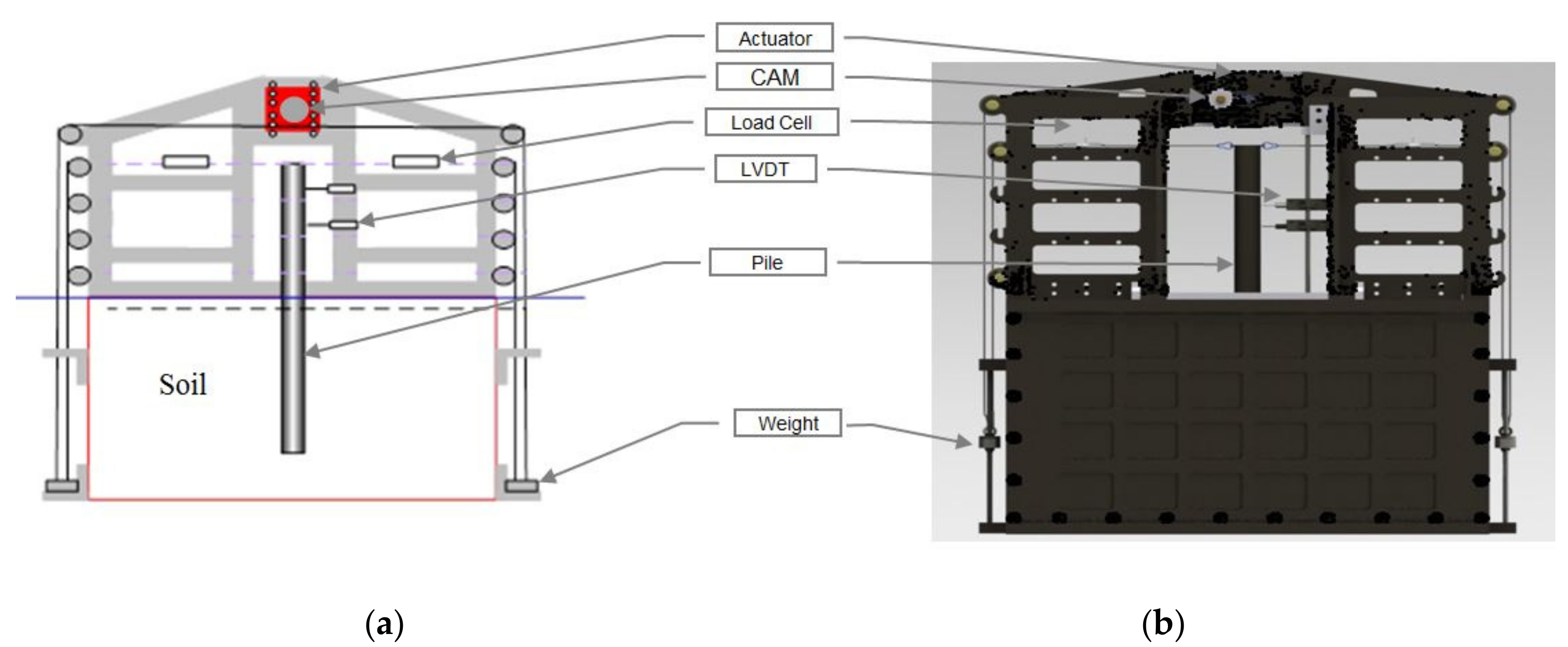
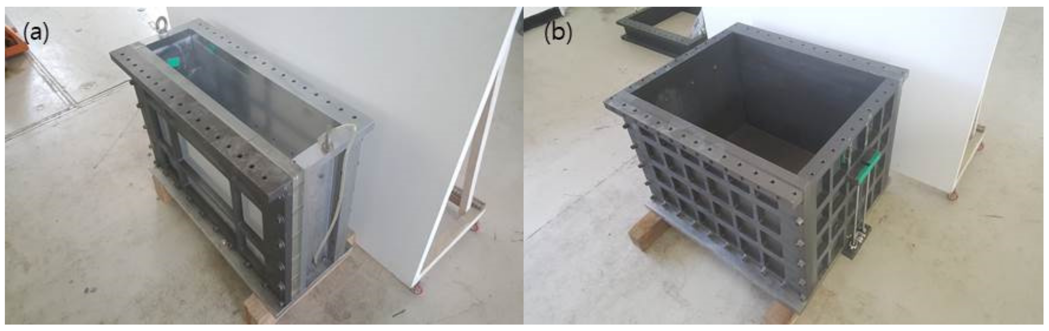
2. Centrifuge Model Test

The rotation radius of the centrifuge model testing device used in the tests was 3 m, and it could accelerate a weight of 11.76 kN to a centrifuge acceleration of 100 g. The gravitational acceleration used in the tests was 94.2 g, considering the weight of the specimens. In the tests, static load tests and cyclic load tests were performed on the monopile. The soil boxes used in the tests had different sizes. This was done in order to consider boundary conditions because load was applied in both directions in the cyclic loading test. As for the soil box’s material, the floor and three sides were made from an aluminum alloy. The front was made from a 4 cm-thick sheet of plastic, which was constructed so that it could be used to view the state of the soil. The soil box used in the static load tests had a length of 80 cm, a width of 20 cm, and a height of 50 cm. The soil box used in the cyclic loading test had a length of 80 cm, a width of 60 cm, and a height of 50 cm. Figure 1 shows the soil box used in the tests.

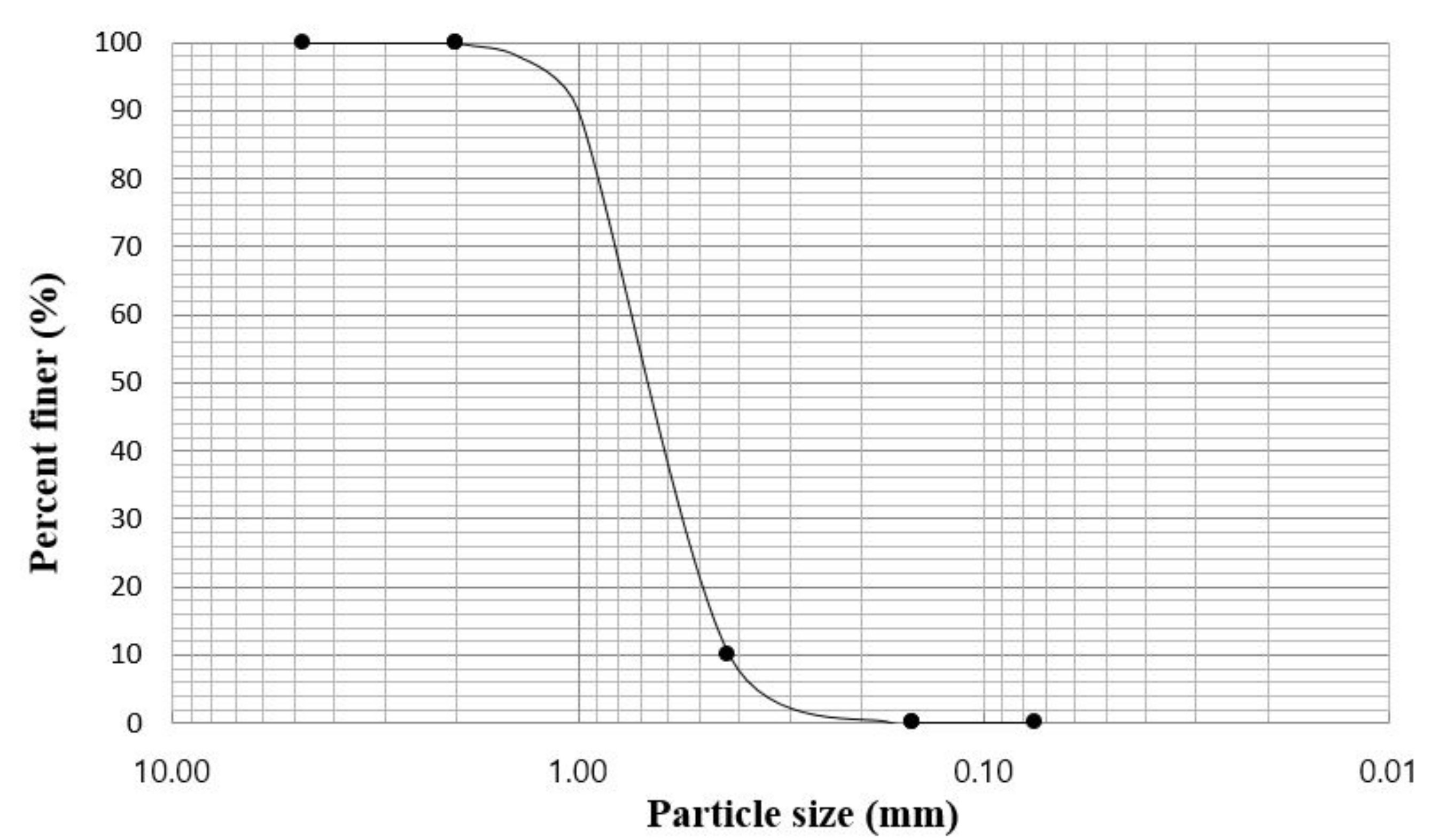
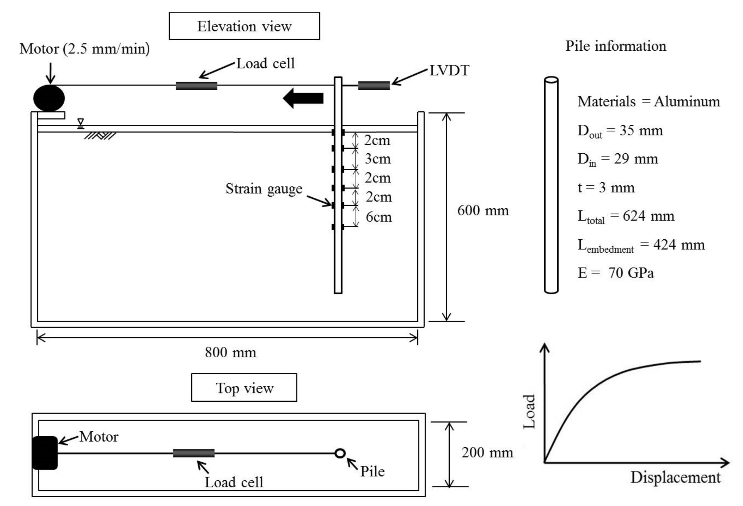
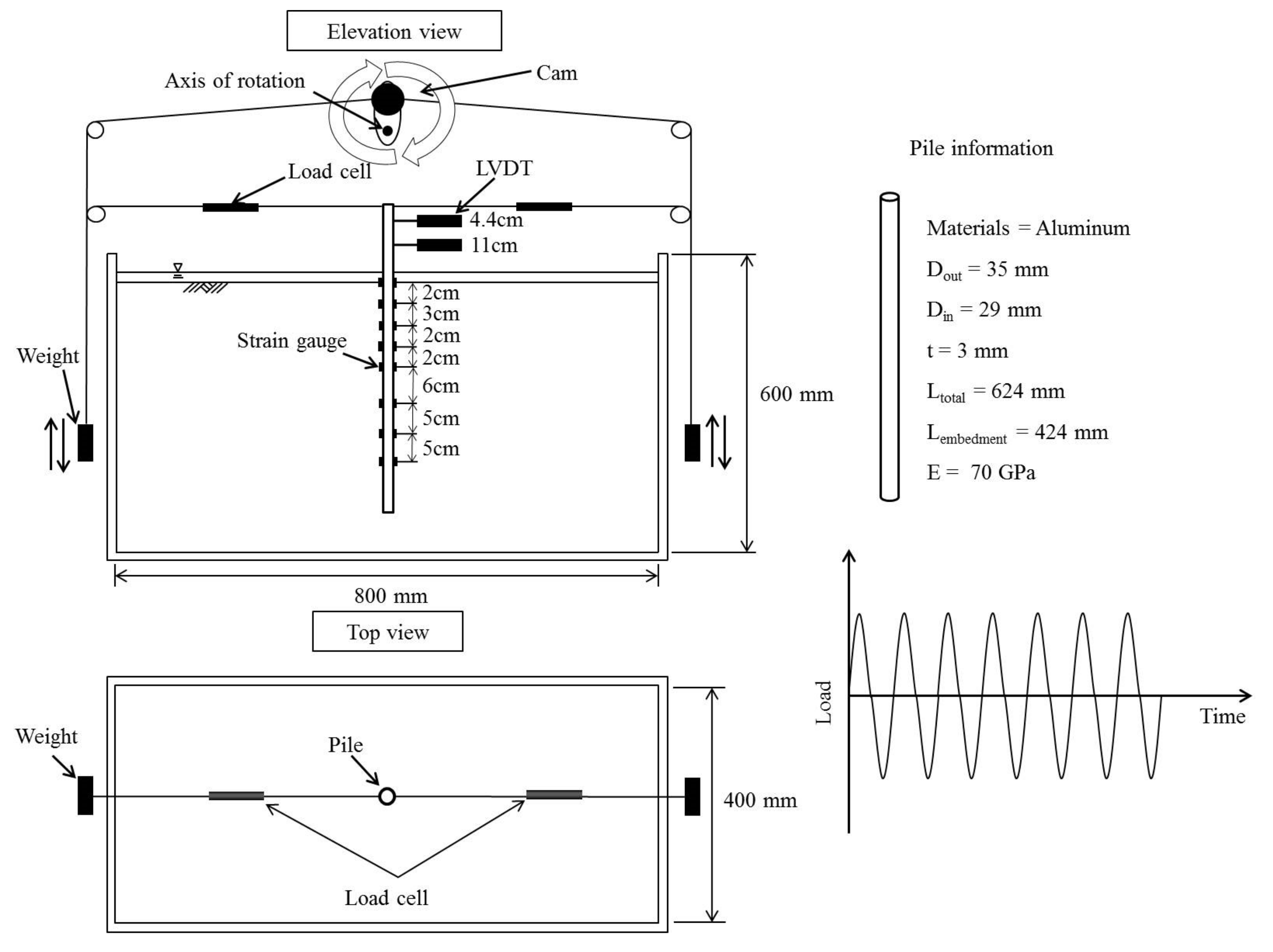
2.1. Soil Properties and Pile Information

The sand used in the composition of the soil was Jumunjin sand, which is classified as SP by the Unified Soil Classification System [16]. Figure 2 shows the particle size distribution curve of the Jumunjin stand. It is important to consider the effect of the soil particle size in centrifuge model tests. Ovesen [17] reported that the specimen particle size has no effect on the pile in centrifuge model tests if the pile diameter is 30 times the effective particle size or more. The diameter of the pile used in this study was around 87 times larger than the effective particle size of Jumunjin sand; therefore, it was considered that there was no particle size effect. The specific gravity (G_s) of the Jumunjin sand used in the experiments was 2.65. The maximum dry unit weight was 16.6 kN/m³. The minimum dry unit weight was 13.3 kN/m³. The internal friction angle was measured as 38° by direct shear testing when the relative density was 80%.

Table 1. Properties of soil.

USCS	SP
Maximum unit weight (kN/m3)	16.6
Minimum unit weight (kN/m3)	13.3
Coefficient of uniformity (Cu)	1.68
Specific gravity (Gs)	2.65
Relative density (%)	80
Friction angle $\left(°\right)$	38

shows the properties of the Jumunjin sand.

As for the material of the pile used in the tests, it was a model monopile made out of aluminum alloy with an elastic modulus of 70 GPa. The model monopile’s total length was 639 mm. It was constructed as an aluminum pipe with a thickness of 3 mm, an outer diameter of 35 mm, and an inner diameter of 29 mm. The model monopile’s insertion depth was 424 mm. Because the tests were performed under a gravitational acceleration of 94.2 g, when the monopile was converted to the original scale, it was modeled as a steel monopile with an insertion depth of 40 m, a total length of 60 m, an outer diameter of 3.3 m, and an inner diameter of 2.7 m. Here, the change in thickness during conversion was calculated to take into account the flexural rigidity. In addition, the relative stiffness, which is one of the most important parameters for lateral pile behavior, was also considered in centrifugal similitude relation. The pile corresponds to a long pile, according to Broms [18]. The pile specification is shown in

Table 2. Pile specification.

	Model Pile	Scale Factor	Prototype Pile
Material	Aluminum	n/a	Steel
Pile length (m)	0.639	λ	60
Embedment depth (m)	0.424	λ	40
Outer diameter (m)	0.035	λ	3.3
Elastic modulus (GPa)	70	1	210
Moment of Inertia (m4)	3.89 × 10–8	λ4	1.02
Flexural rigidity (kN∙m2)	2.73	λ4	2.15 × 108
Load (N)	1.0	λ	8873.6
Relative stiffness (-)	2.04 × 10–4	1	2.07 × 10–4

.

2.2. Static Loading Test

Figure 3 shows a cross section of the test, including the measuring device used in the test. To analyze the behavior of the pile according to depth, strain gauges were attached to 12 places on both sides of the pile at depths from the surface of 0, 2, 5, 7, 9, and 15 m. A Linear Variable Differential Transformer (LVDT) and load cell were installed at the top of the model pile to measure the displacement and load at the pile head. In the static loading test, a wire that was connected to a motor and the model monopile head was pulled, and the displacement was controlled at a fixed speed (2.5 mm/min). The effect of the soil boundary was considered, and a space of more than 10 times the pile diameter was reserved in the direction in which the monopile was being loaded. This corresponds to a study by Remaud [19], which states that the pile and boundary do not affect each other at a distance of more than 10 times the pile diameter.

Table 3. Static loading test conditions.

Case	Penetration Depth (mm)	Motor Speed (mm/min)	Relative Density (%)
S-80	424	2.5	80

shows the test conditions for the static loading test. In the term “S-80” that is used here, the “S” stands for static loading test, and the “80” refers to the soil relative density. The soil’s relative density was made to be 80% using a sand raining technique to create a uniform soil.

2.3. Cyclic Loading Test

The cyclic loading system, which can endure centrifuge acceleration, was designed based on the system studied by Peng et al. [20]. The cyclic loading system’s design was improved to be able to withstand gravitational acceleration in the centrifuge model tests, as shown in Figure 4a. Weights hanging from both sides can be independently adjusted to create a variety of loads. Finally, a cam method was used to adjust the rotational speed according to the cam’s movement to be able to adjust the period of the cycle. Figure 4b shows the cyclic lateral loading device used in the centrifuge model tests.

Figure 5 shows a cross section which includes the measurement device used in the cyclic loading test. To analyze the behavior of the pile at the same depth as the static loading test, 16 strain gauges were attached on both sides at buried depths of 0, 2, 5, 7, 9, 15, 20, and 25 m. In the tests, two LVDTs and two load cells were installed on the model monopile head to measure the cyclic lateral load and the displacement. To reduce the effect of the soil’s boundary surface at this time, the distance between the soil box and the pile was made to be more than 10 times the pile diameter.

Table 4. Cyclic loading test conditions.

Case	Embedment Depth (mm)	Load (kN)	Frequency (Hz)	Relative Density (%)
C-1416	424	1416	0.125	80
C-2361		2361
C-3777		3777
C-5666		5666

shows the test conditions for the cyclic loading test. In the “C-80-1416” shown here, “C” means cyclic loading test; “80” means the soil’s relative density (%); and “1416” means the size of the cyclic lateral load (kN) in prototype scale. The rest of the case names have similar meanings. As for the cyclic loading test soil composition, a sand pluviator was used in the same manner as the static loading test soil composition method to make the relative density 80%. The cyclic loading period was set at 0.125 Hz so that a single cycle of the cam’s circular motion occurred over a duration of 8 s. The ultimate load found in the static loading test was used as the cyclic load size. Four loads were calculated at 30%, 50%, 80%, and 120% of the ultimate load, and the tests were performed.

3. Centrifuge Model Test Results

3.1. Selecting the Ultimate Load

Figure 6 shows a graph of the lateral load and displacement of the pile head in the static loading test. The lateral bearing capacity was found from the displacement at a pile diameter of 10%, as suggested by Fleming et al. [21], and it was determined to be 4722 kN. The experiment results presented here are shown using the scale ratios in Table 1.

3.2. The p-y Curve Creation Method

The average value of the strain rate ($\mathsf{\epsilon }$) measured from the strain gauges attached to both sides of the pile at each depth was used to find the moment at each pile depth and create a distribution curve. The beam theory equation shown in Equation (1) was used to calculate the soil resistance p and the pile displacement y. Cubic spline interpolation was used as the method for this process [22].

To find the soil resistance p, the second derivative of the moment curve must be found according to depth. To find the pile displacement y, the moment must be divided by the flexural rigidity, and the double integral must be found.

$$p=\frac{d^2}{d{z}^2}M\left(z\right),y=\iint \frac{M\left(z\right)}{EI}$$

(1)

Here, p is the soil resistance (F/L); y is the pile displacement (L); EI is the pile flexural rigidity (F∙L²); and M(z) is the moment distribution curve according to depth (F∙L).

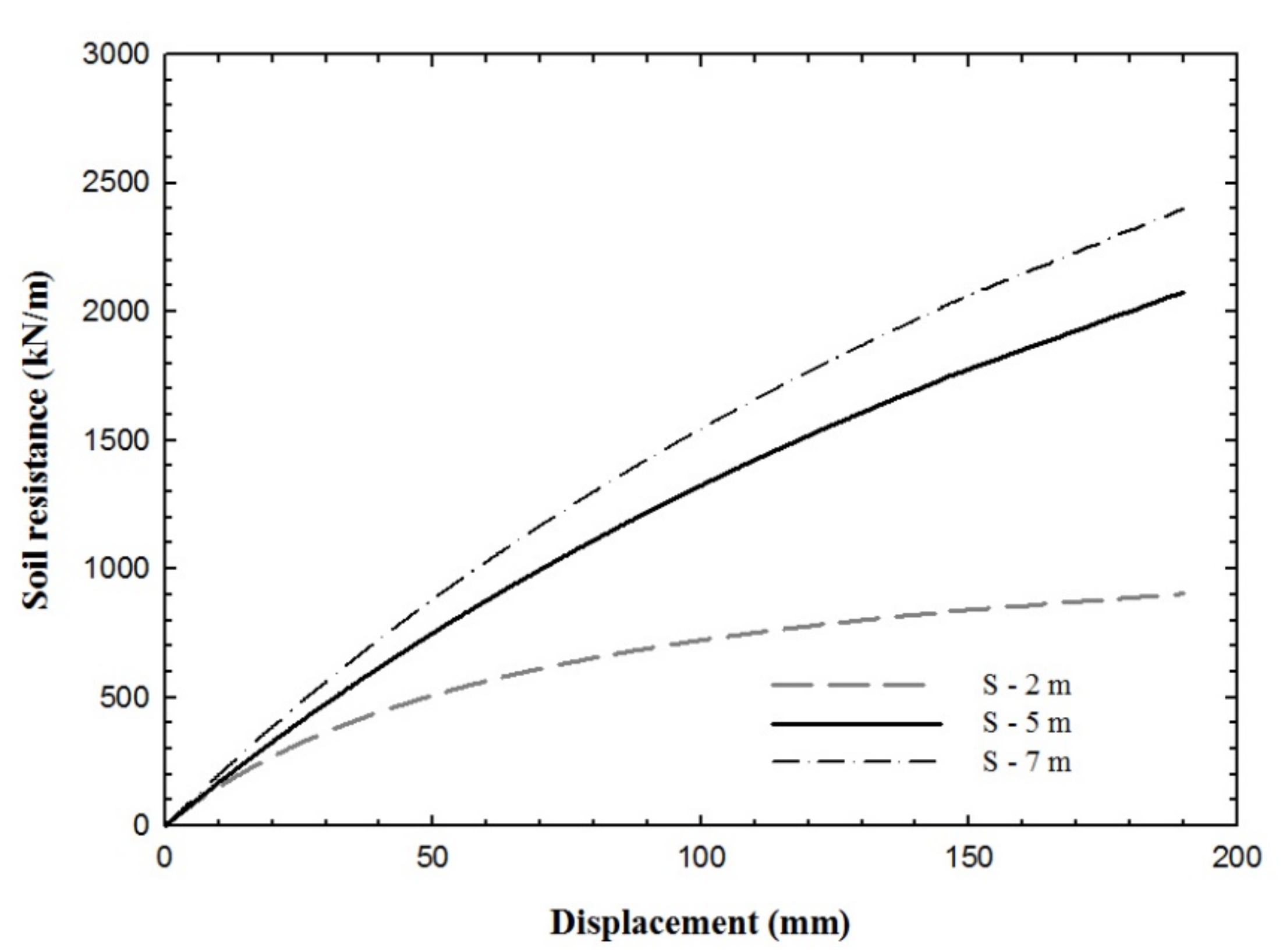
3.3. Experimental Static p-y Curve Results

Figure 7 shows the static p-y curve at various depths. This was back-calculated from the bending moment in the pile. The bending moment was obtained from the attached strain gauge. After this, the static p-y curve was found, as described in Section 3.2. From the static p-y curve, it was found that as the depth increases, the initial modulus of subgrade reaction (k_ini) and ultimate soil resistance (p_u) increase, and this appears in the form of a hyperbolic curve. In Figure 6, the pile showed elastic behavior in the range of destruction, but in Figure 7 the soil was destroyed and began to yield.

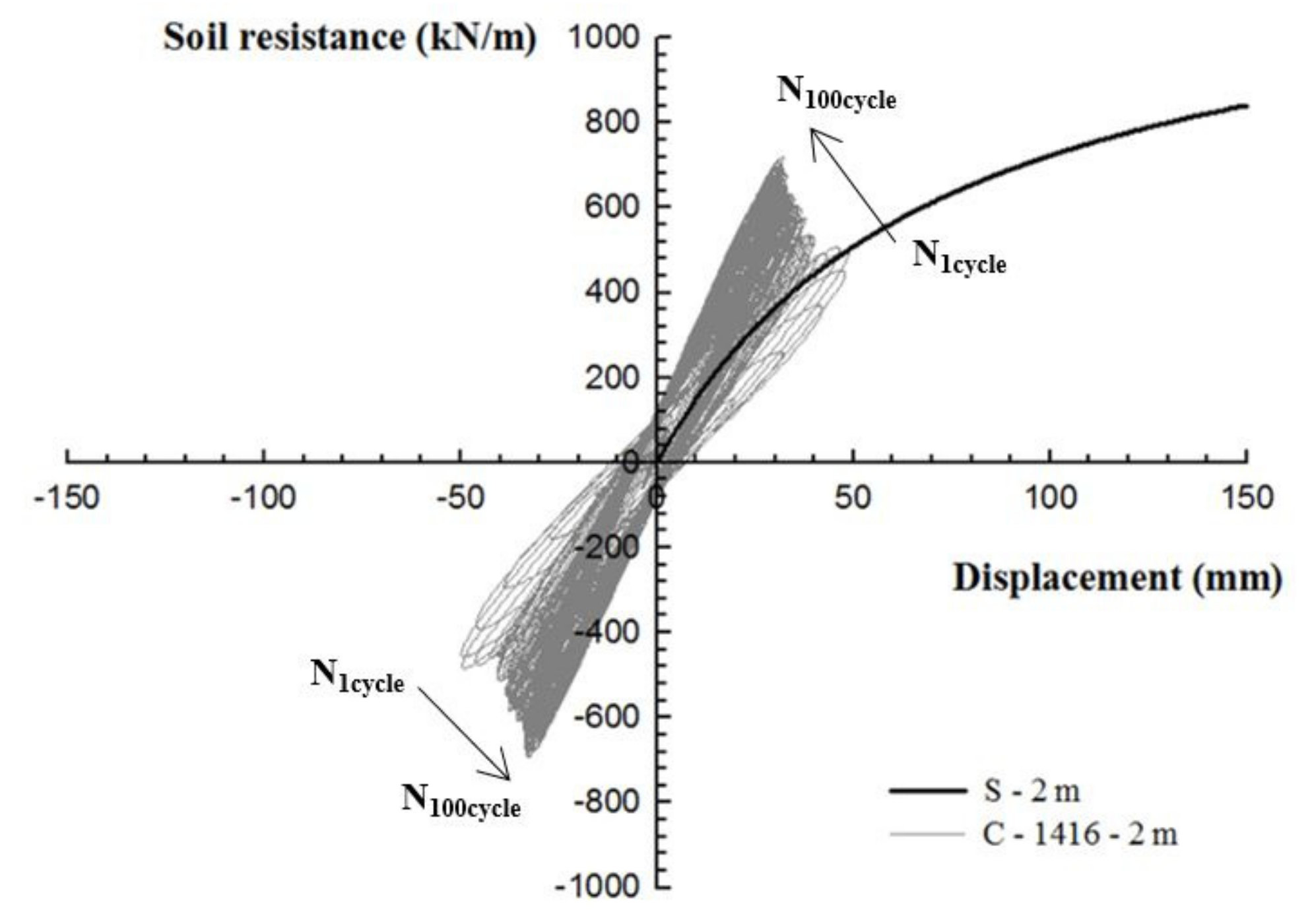
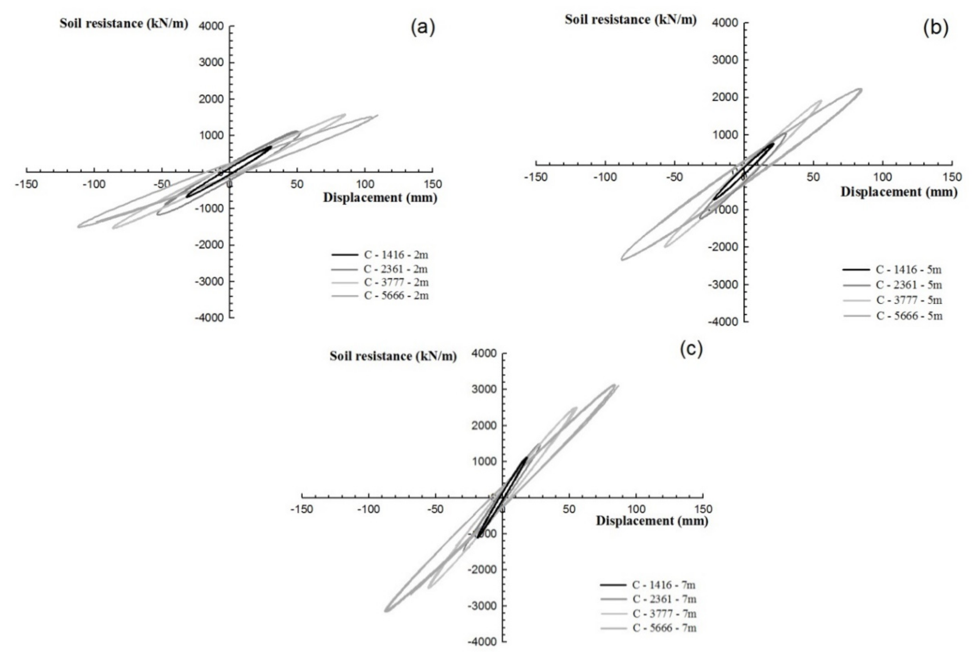
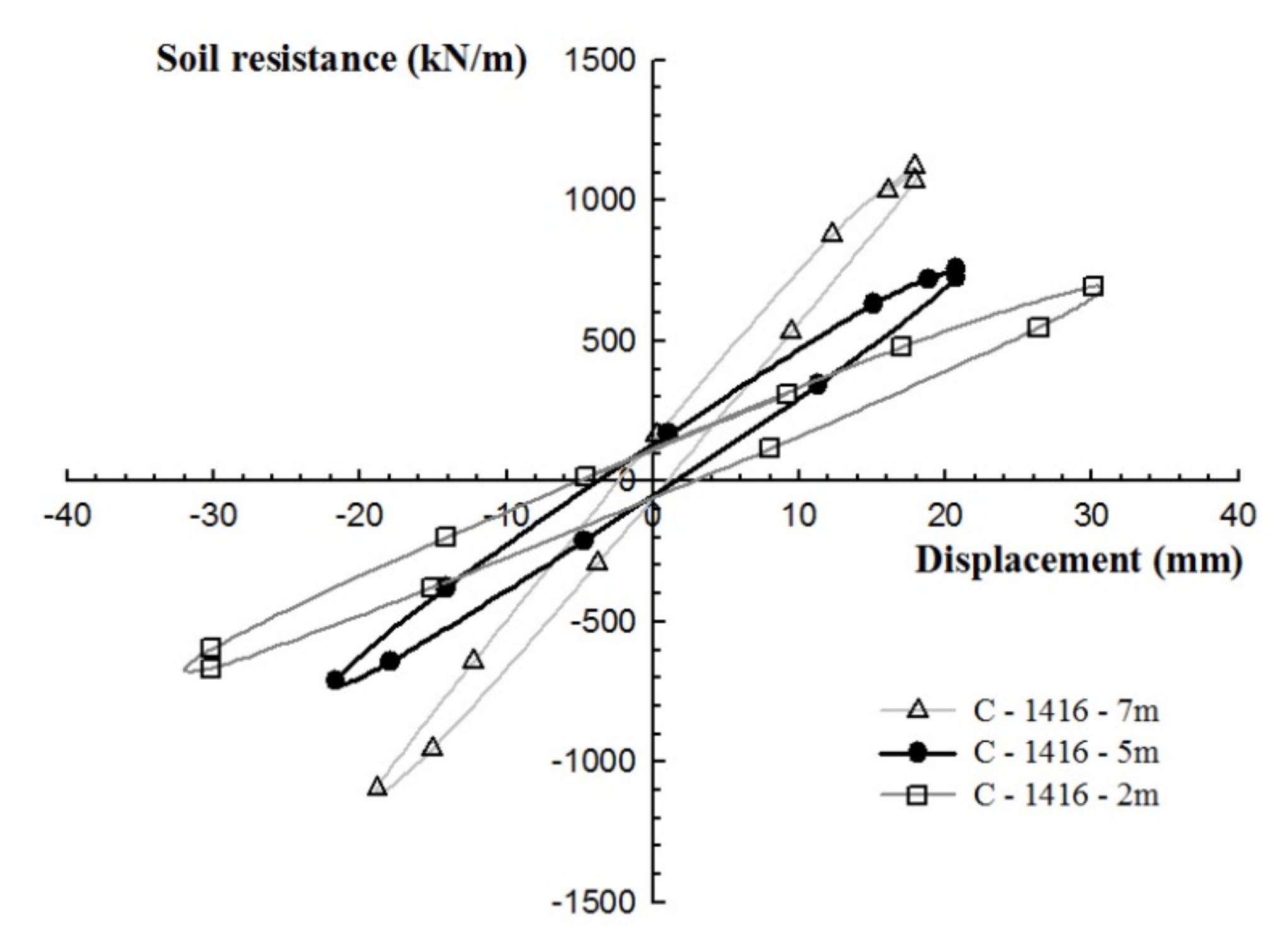
3.4. Experimental Cyclic p-y Curve Results

The cyclic p-y curves for each depth were found from the values measured by the strain gauge at each buried depth. Figure 8 shows the experimental cyclic p-y curve and the experimental static p-y curve at a depth of 2 m, as calculated using Equation (1). The results show that there was a similar trend in the experimental cyclic p-y curve for the first cycle and the static p-y curve. However, as the number of cycles increased, the soil resistance in the experimental cyclic p-y curve tended to increase, while the pile displacement tended to gradually decrease. At the front of the pile, loading and unloading occurred due to the cyclic load. Nearby sand filled the gaps between the soil and the pile, which occurred during unloading. As the gaps that were filled by nearby sand became denser due to cyclic loading, the soil resistance increased, and it was found that the displacement tended to decrease. Research results that are similar to this have also been reported by Møller and Christiansen [2], Qin and Guo [23], and Rosquoet et al. [24].

Figure 9 shows the p-y curve by depth for 100 cycles during cyclic loading. The results show that as the depth increases, the displacement tends to decrease, and the soil resistance tends to increase. This was found to match the trend in which the strength of the soil tends to increase as the depth increases.

Figure 10 shows the soil resistance according to the number of cycles. A total of 100 cycles were used and it was possible to determine the soil resistance according to the increase in cycles. As the number of cycles increased, the soil resistance increased, but the soil resistance showed a tendency towards convergence after 90 cycles. It was found that the number of cycles affects the soil resistance, but after 90–100 cycles, the soil resistance converges, and the number of cycles has little effect on the soil resistance.

Figure 11 shows the cyclic p-y curve for each load at depths of 2, 5, and 7 m. Four kinds of cyclic loading were performed, and the results were found for the 100th cycle. It was found that the pile displacement and soil resistance tended to increase as the cyclic loading increased and that the initial stiffness and soil resistance increased as the depth increased. At 30% and 50% of the ultimate load, the modulus of subgrade reaction was fixed and showed no changes, but at 120% of the ultimate load, the modulus of subgrade reaction decreased. At a depth greater than 7 m, it was possible to obtain data, but this was excluded from the analysis. The reason for this is that the soil resistance and pile displacement analysis results did not seem to be meaningful. Furthermore, because it was the behavior of a long pile, it was determined that there was no effect in deep places.

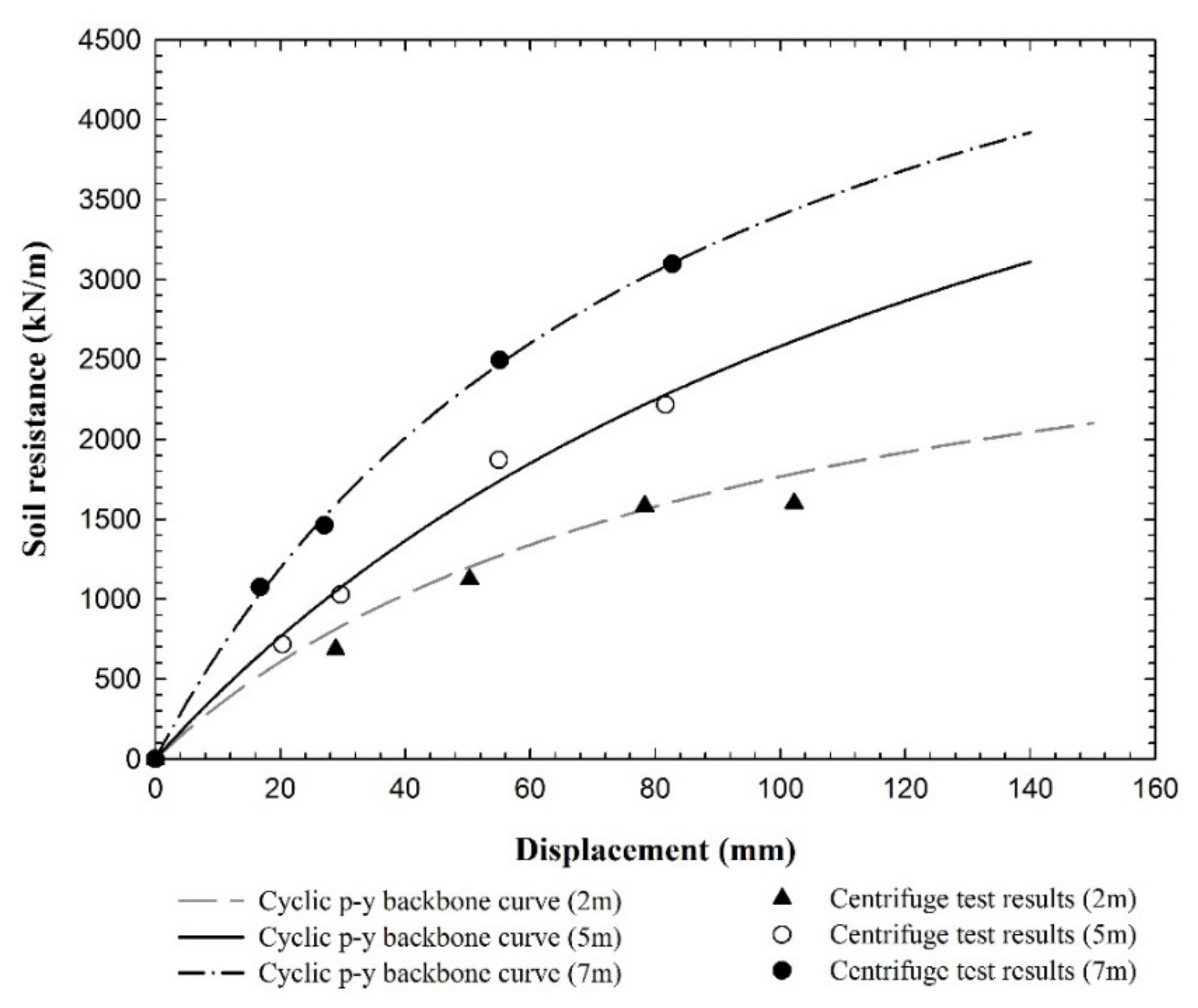
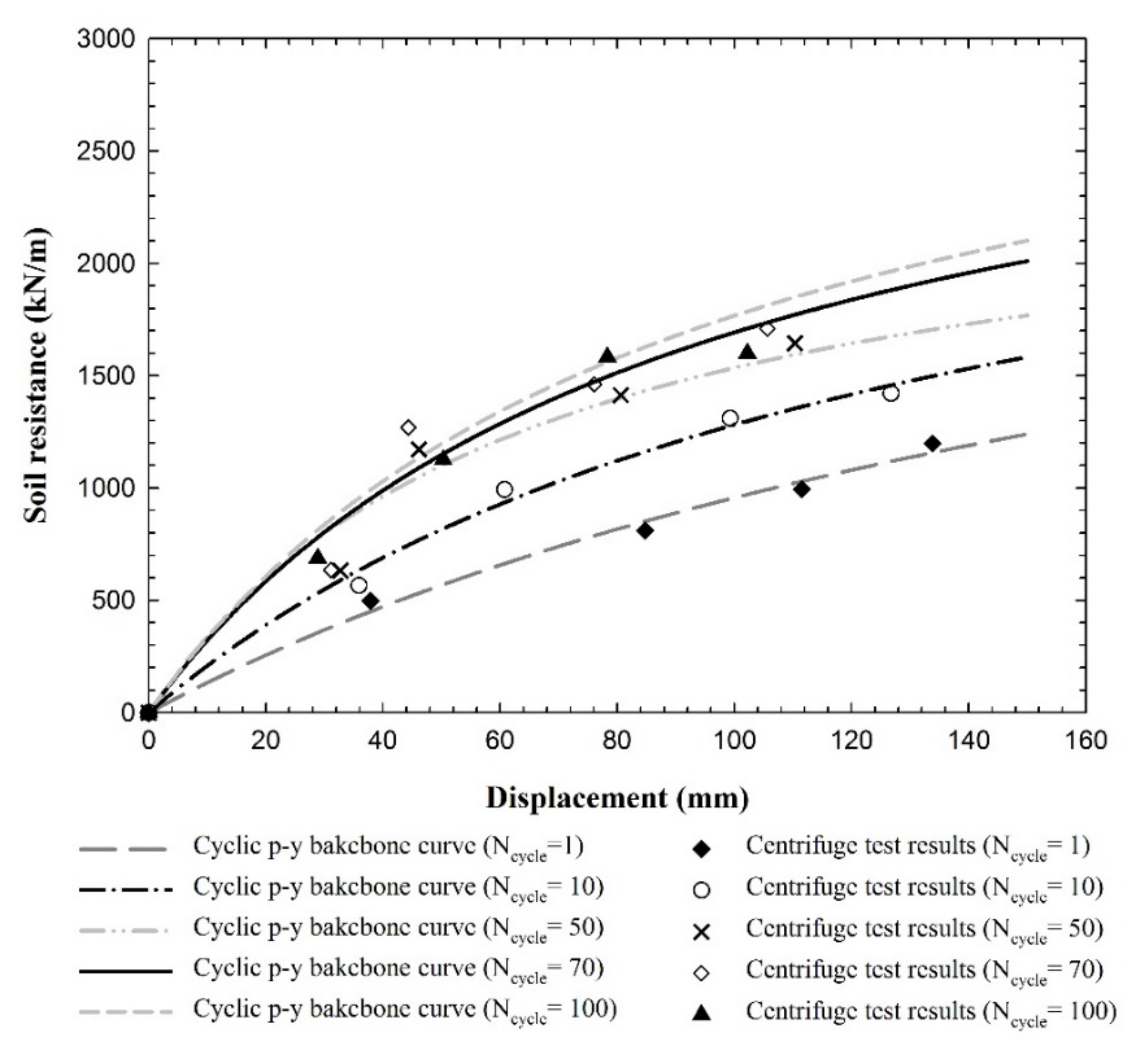
4. Cyclic p-y Backbone Curve for Dry Sand

This study has aimed to use the cyclic p-y curve to propose a cyclic p-y backbone curve that can be put to practical use when making designs related to cyclic loading of large-caliber monopiles that can be used in foundations. The cyclic p-y curve was determined by calculating the maximum soil resistance points found in the tests and connecting these points to find the cyclic p-y curve [25,26,27].

Figure 12 shows the cyclic p-y backbone curve at depths from the ground surface. The backbone curve was fitted by using a hyperbolic curve formula on the maximum soil resistance and pile displacement at the 100th cycle. Because the maximum soil resistance converges at the 100th cycle, it was assumed that the pile long-term behavior was shown at the 100th cycle. The equation used to find the backbone curve was Equation (2), which is a hyperbolic curve equation suggested by [28].

$$p=\frac{y}{\frac{1}{k_{ini}}+\frac{y}{p_u}}$$

(2)

Here, p_u is the ultimate soil resistance (F/L); k_ini is the initial modulus of subgrade reaction (F/L³); and y is the pile displacement (L).

Figure 13 shows the cyclic p-y backbone curve at a depth of 2 m, according to the number of cycles. The cyclic p-y backbone curve was found for 1, 10, 50, 70, and 100 cycles. It was found that, as the number of cycles approached 100, the cyclic p-y backbone curve showed a tendency to converge.

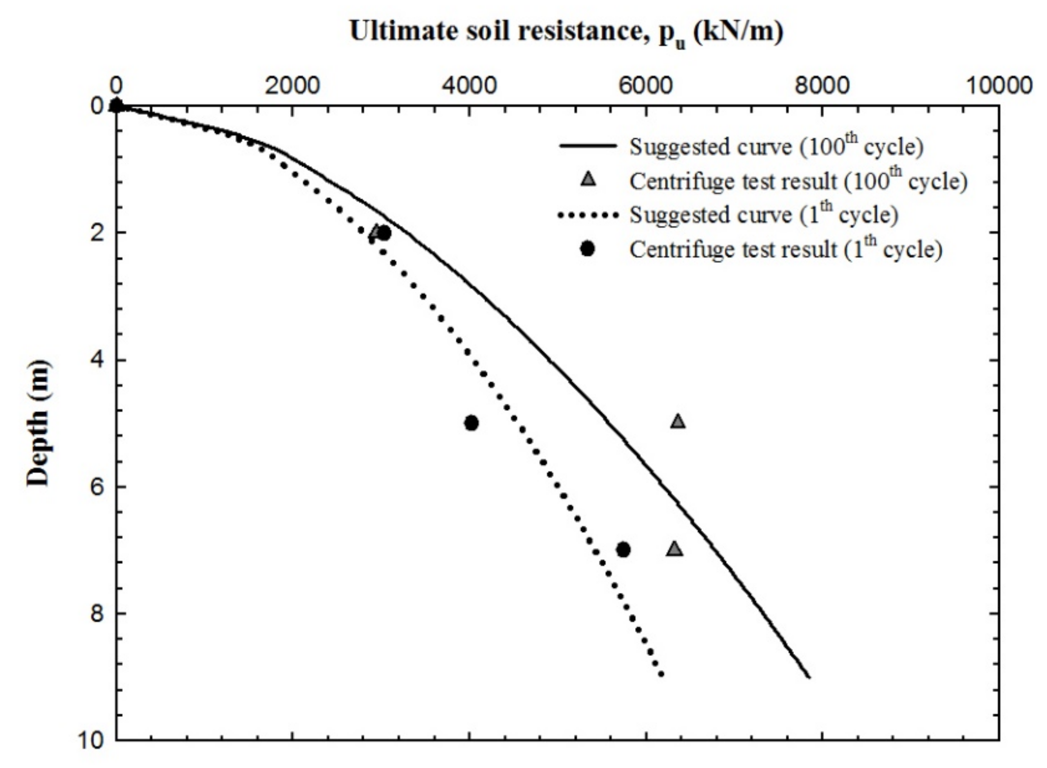
4.1. Ultimate Soil Resistance (p_u)

Ultimate soil resistance increases according to depth, but it is not clear by how much. There is also no clear trend regarding whether it increases nonlinearly or linearly. Therefore, this study used Equation (3) and fitted the test data to the ultimate soil resistance curve according to depth. Equation (3) has been used by several researchers [27,29,30] and it is a modification of an equation by Broms [18].

$$\frac{p_u}{D}=\mathrm{A}{K}_p\gamma z^n$$

(3)

Here, $K_p$ is the Rankine passive earth pressure coefficient; $\mathrm{A}\mathrm{and}n$ are the regressive analysis constants; $\gamma$ is the unit weight (F/L³); $z$ is the depth (L); and D is the pile diameter (L).

In the equation by Broms [18], the fitting parameter A is 3 and passive soil pressure is assumed, i.e., n = 1. As such, the ultimate soil resistance increases linearly according to depth. However, API [8] suggested that it increases nonlinearly according to depth. In this study, two fitting parameters, A and n, were used for the sake of the equation’s flexibility, and the ultimate soil resistance according to depth was nonlinear. Fitting parameters were found in order to find the equations for the ultimate soil resistance by depth for the first cycle and the ultimate soil resistance by depth for the 100th cycle. As a result, the fitting parameters A and n for the first cycle were 9.02 and 0.53, respectively. The fitting parameters A and n for the 100th cycle were 10.2 and 0.58, respectively.

Figure 14 shows the ultimate soil resistance by depth for the first and 100th cycles, using the fitting parameters A and n, which were found previously. Over a depth of 1 m, the difference in the ultimate soil resistance due to the number of cycles was negligible, but as depth increased, it was found that a large difference in ultimate soil resistance occurred.

4.2. Initial Modulus of Subgrade Reaction (k_ini)

The initial modulus of subgrade reaction, k_ini, also increases according to depth. Equation (4) below shows the initial modulus of subgrade reaction.

$$k_{ini}=n_{h}z$$

(4)

Here, $k_{ini}$ is the initial modulus of subgrade reaction (F/L²); $n_h$ is the modulus of subgrade reaction constant (F/L³); and $z$ is the depth (L).

Equation (4) was suggested by [31] to analyze lateral load tests, and [32] reported that it is proportional to depth. However, there is a dispute over whether the initial modulus of subgrade reaction is affected by the pile diameter. Nonetheless, not only did API [8] use a fixed value, a study by Ashford and Juirnarongrit [33] reported that the initial modulus of subgrade reaction is unrelated to the pile diameter. Hence, Equation (4) was used in this study.

Figure 15 shows the initial modulus of subgrade reaction by depth for the first and 100th cycles. The modulus of subgrade reaction was back-calculated using Equation (4). The results showed that the modulus of subgrade reaction for the first cycle was 6228 kN/m³, and the modulus of subgrade reaction for the 100th cycle was 10,313.4 kN/m³. It was found that the modulus of subgrade reaction for the 100th cycle was 65% larger than the modulus of subgrade reaction for the first cycle. This confirmed that the initial modulus of subgrade reaction increases as the number of cycles increases.

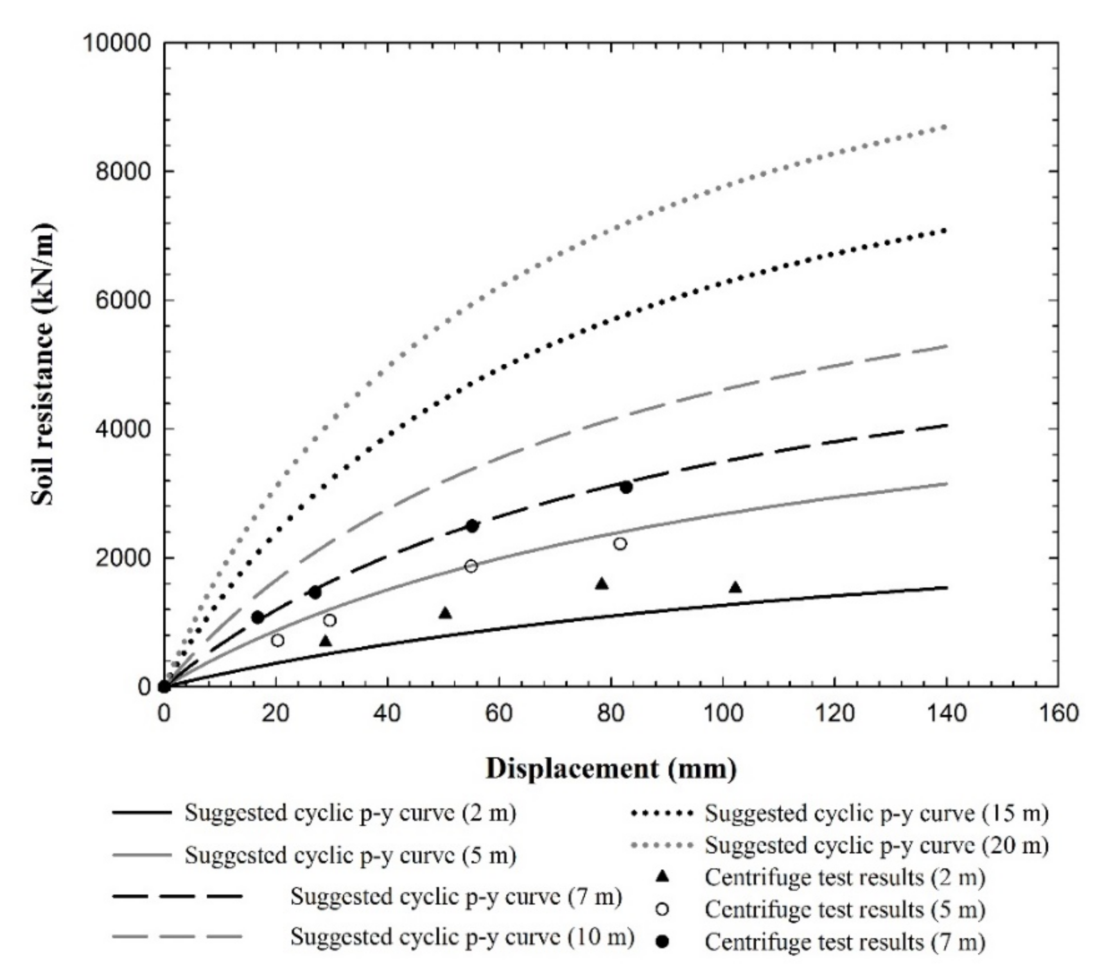
4.3. Suggested Cyclic p-y Curve

Figure 16 and Figure 17 show the cyclic p-y curves for the first and 100th cycles at various depths. To verify the centrifuge model test results, the centrifuge model test data for depths of 2, 5, and 7 m are also shown. As shown in Figure 16, there is a small error between the suggested cyclic p-y curve at 5 m and the centrifuge model test results. However, aside from this, the suggested cyclic p-y curves strongly match the test results. Also, it is shown that the initial modulus of subgrade reaction and the ultimate soil resistance tended to increase according to depth, and this is believed to strongly show the characteristics of the soil response. The suggested cyclic p-y curve is only a curve for dry soil. In case of saturated soil, the p-y curve should be established respectively. The suggested cyclic p-y curve for the first cycle can show the lower limit, and the soil resistance converges at the 100th cycle so that the suggested cyclic p-y curve for the 100th cycle can show the upper limit. Therefore, the first cyclic p-y curve was named the lower limit cyclic p-y curve and the 100th cyclic p-y curve was named the upper limit cyclic p-y curve.

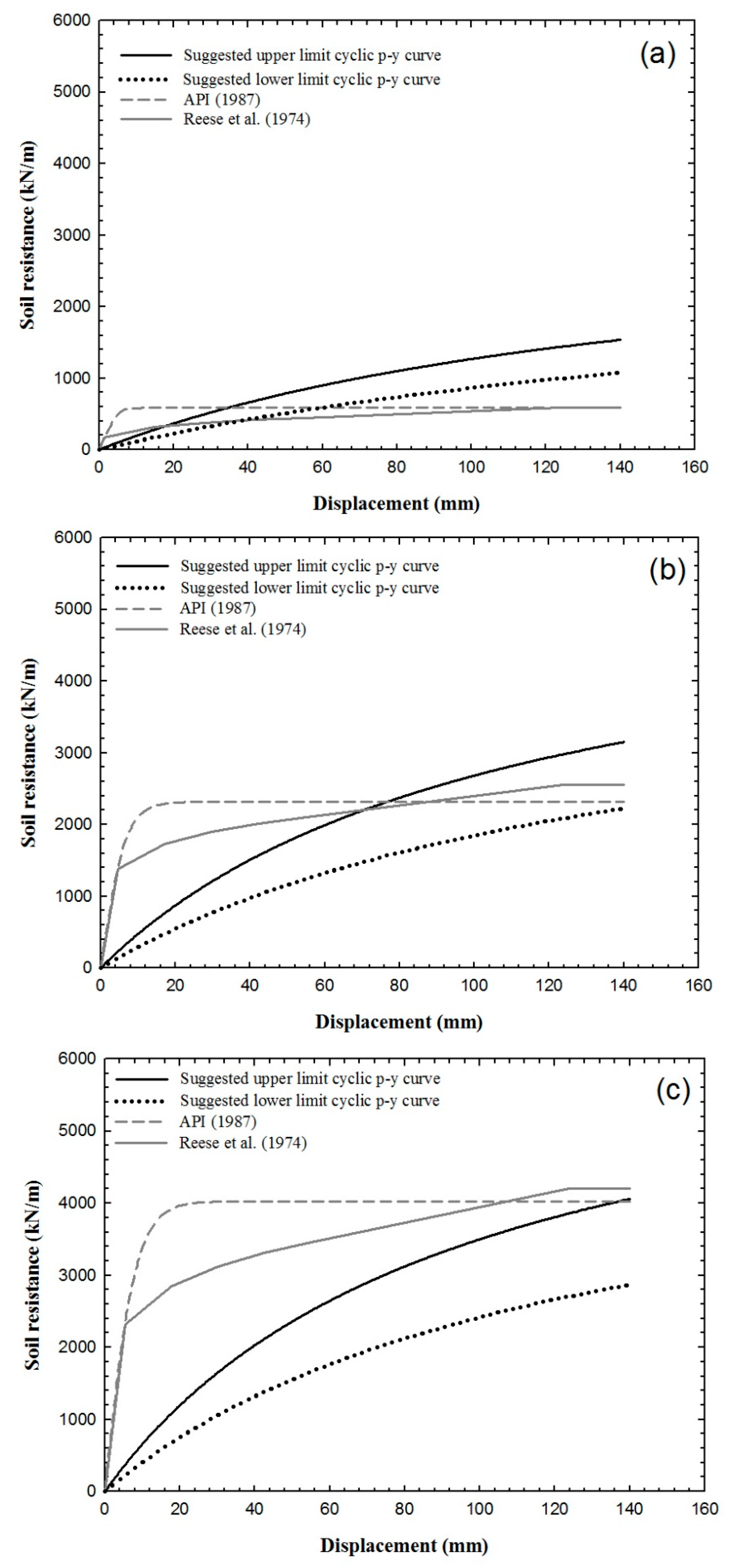
5. Comparison with Existing p-y Curves

Figure 18 show a comparison of the suggested upper limit cyclic p-y curve and the lower limit cyclic p-y curve with the existing p-y curve. For the existing p-y curve, the API [8] and Reese et al. [11] methods were used. The biggest difference between the suggested cyclic p-y curve and the existing p-y curve was the pile displacement, which occurs when the maximum soil resistance occurs. In the case of the API [8] cyclic p-y curve, the ground reaction rapidly increased until a pile displacement of 10–15 mm was reached, after which it converged at the maximum ground reaction. On the other hand, in the case of the suggested cyclic p-y curve, nonlinear behavior occurred as the pile displacement increased, and the ground reaction gradually increased. The reason for this is that the initial soil resistance has a big effect on the shape of the p-y curve, and the Jumunjin sand initial soil resistance is smaller than in the API method. Therefore, the aforementioned difference was seen. As for the maximum ground reaction, the suggested upper limit cyclic p-y curve was larger than the existing p-y curve. The API [8] method is one of the most widely used methods for the seafloor, but there are many studies which report that it overestimates the initial modulus of subgrade reaction for piles of a larger caliber [13,30,34]. In addition, Yoo et al. [15] reported test results that were up to 80% smaller than the API [8] modulus of subgrade reaction. The suggested cyclic p-y curve is based on the soil properties and pile diameter. However, for the API cyclic p-y curve, the API static p-y curve is multiplied by a correction factor of 0.9 to obtain the calculated curve.

According to test results on piles exposed to cyclic loading, the cyclic p-y curves converge as the number of cycles increases, but the shape of the cyclic p-y curves vary during the initial cycles (1–90). If short-term behavior is considered, the cyclic p-y curve’s upper and lower limit must be considered and applied in design.

6. Conclusions

This study used a centrifuge model test device to conduct tests on the lateral behavior of a monopile with a diameter of 3.3 m, which was inserted in dry sand with a relative density of 80%. A single static loading test and four cyclic loading tests were performed. The cyclic loading was done at 30%, 50%, 80%, and 120% of the static load, and 100 cycles were performed. Using the centrifuge model test results, a regression analysis was performed on the soil resistance and the initial modulus of subgrade reaction to find the suggested formula. From this, the upper limit cyclic p-y curve and the lower limit cyclic p-y curve by depth were formulated. The following conclusions were obtained, based on the test results and the suggested cyclic p-y curve:

(1)

The first cycle cyclic p-y curve showed tendencies that were similar to the static p-y curve. As the number of cycles increased, the initial slope and soil resistance increased. This was found to be due to a phenomenon in which nearby soil filled the gap between the pile and the sand and became denser due to cyclic loading;

(2)

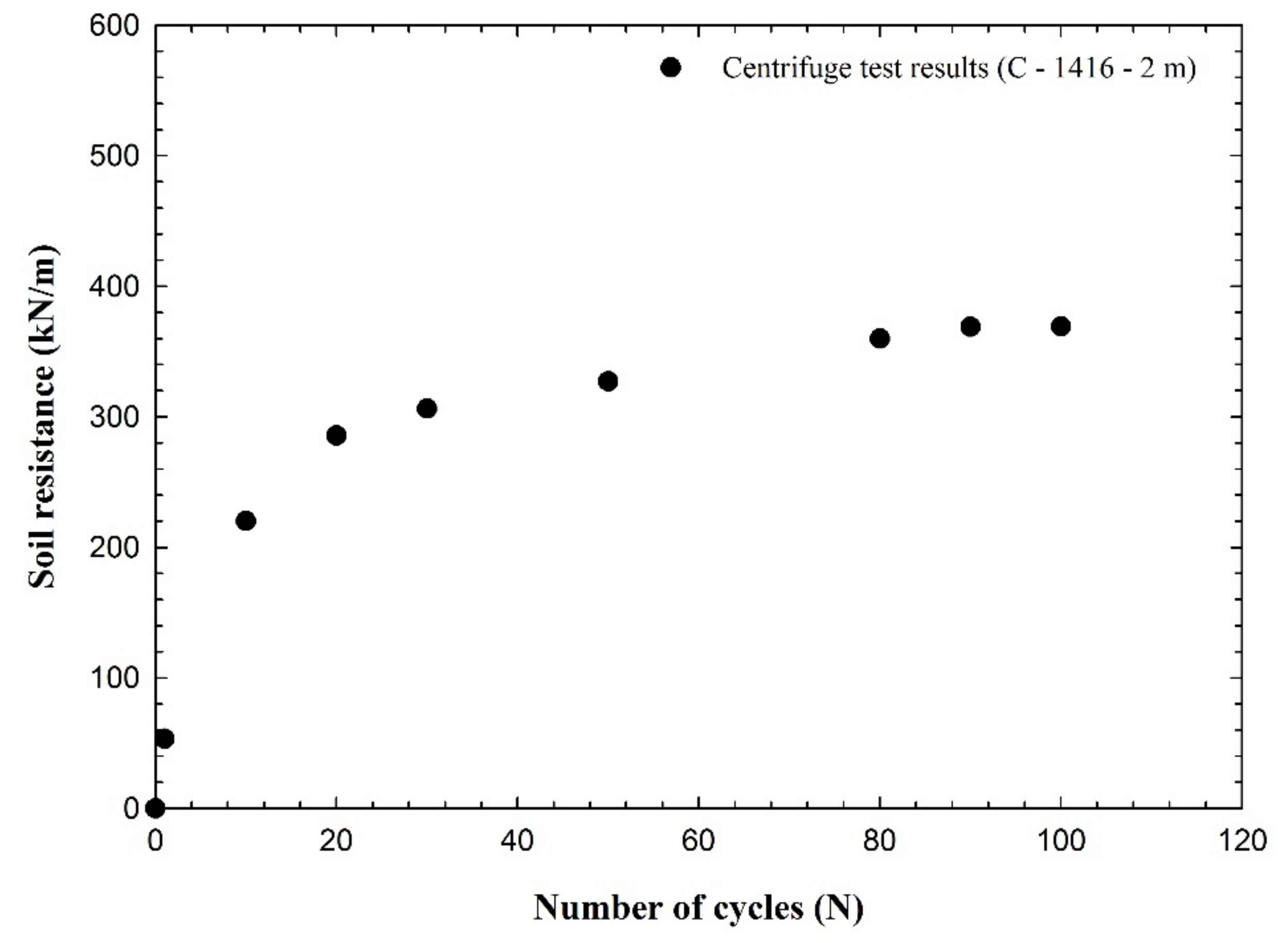
The cyclic p-y backbone curve followed the increase in the number of cycles. It tended to increase from the first to the 90th cycle and converge from the 90th to the 100th cycle. This was found to be an effect of the initial number of cycles on the cyclic p-y curve;

(3)

The initial modulus of subgrade reaction was assumed to increase nonlinearly, according to depth, and a regression analysis was performed on it to find the modulus of subgrade reaction. The results showed that the modulus of subgrade reaction after the first cycle was 6228 kN/m³, and the modulus of subgrade reaction after the 100th cycle was 10,313.4 kN/m³;

(4)

As for the maximum soil resistance, the suggested cyclic p-y curve was greater than the API p-y curve [8]. However, in the API p-y curve, the soil resistance converged at a pile displacement of 10–15 mm, while in the suggested cyclic p-y curve, the soil resistance showed a tendency to gradually increase according to an increase in the pile displacement;

(5)

The upper and lower limit of the cyclic p-y curve according to the number of cycles was found. The shape of the cyclic p-y curve varies from the first to the 100th cycle; therefore, further research on this phenomenon is necessary when short-term behavior is considered;

References

1. Achmus, M.; Kuo, Y.-S.; Abdel-Rahman, K. Behavior of monopile foundations under cyclic lateral load. Comput. Geotech. 2009, 36, 725–735. [Google Scholar] [CrossRef]
2. Møller, I.F.; Christiansen, T. Laterally Loaded Monopile in Dry and Saturated Sand—Static and Cyclic Loading; Aalborg University: Aalborg, Denmark, 2011. [Google Scholar]
3. Kim, K.; Nam, B.H.; Youn, H. Effect of Cyclic Loading on the Lateral Behavior of Offshore Monopiles Using the Strain Wedge Model. Math. Probl. Eng. 2015, 2015, 1–12. [Google Scholar] [CrossRef]
4. Peralta, P. Investigations on the Behavior of Large Diameter Piles under Long-Term Lateral Cyclic Loading in Cohesionless Soil. Ph.D. Thesis, Leibniz University, Hannover, Germany, 2010. [Google Scholar]
5. Roesen, H.R.; Ibsen, L.B.; Andersen, L.V. Small-Scale Testing Rig for Long-Term Cyclically Loaded Monopiles in Cohesionless Soil. In Proceedings of the Nordic Geotechnical Meeting Nordic Geotechnical Meeting, Copenhagen, Denmark, 9–12 May 2012; pp. 435–442. [Google Scholar]
6. Gerber, T.M.; Rollins, K.M. Cyclic P-Y Curves for a Pile in Cohesive Soil. In Geotechnical Earthquake Engineering and Soil Dynamics Congress IV; ASCE: Sacramento, CA, USA, 2008; pp. 1–10. [Google Scholar]
7. Fan, C.-C.; Long, J.H. Assessment of existing methods for predicting soil response of laterally loaded piles in sand. Comput. Geotech. 2005, 32, 274–289. [Google Scholar] [CrossRef]
8. American Petroleum Institute. Recommended Practice for Planning, Designing, and Constructing Fixed Offshore Platforms; American Petroleum Institute: Washington, DC, USA, 1987. [Google Scholar]
9. Matlock, H. Correlations for Design of Laterally Loaded Piles in Soft Clay. In Offshore Technology in Civil Engineering’s Hall of Fame Papers from the Early Years; ASCE: Sacramento, CA, USA, 1970; Volume 1, pp. 77–94. [Google Scholar]
10. Cox, W.R.; Reese, L.C.; Grubbs, B.R. Field Testing of Laterally Loaded Piles in Sand. In Proceedings of the Offshore Technology Conference, Houston, TX, USA, 6–8 May 1974. [Google Scholar]
11. Reese, L.C.; Cox, W.R.; Koop, F.D. Analysis of Laterally Loaded Piles in Sand. 80OTC 1974, 2, 473–483. [Google Scholar]
12. Brown, D.; O’Neill, M.; Hoit, M.; McVay, M.; El Naggar, M.; Chakraborty, S. Static and Dynamic Lateral Loading of Pile Groups. NCHRP Report 461. National Cooperative Highway Research Board. In Transportation Research Board, National Research Council; Transportation Research Board: Washington, DC, USA, 2001. [Google Scholar]
13. Choo, Y.W.; Kim, D.W. Experimental Development of the P-Y Relationship for Large-Diameter Offshore Monopiles in Sands: Centrifuge Tests. J. Geotech. Geoenvironmental Eng. 2015, 142, 04015058. [Google Scholar] [CrossRef]
14. Li, Z.; Haigh, S.; Bolton, M. Centrifuge modelling of mono-pile under cyclic lateral loads. Phys. Model. Geotech. Two Vol. Set 2010, 2, 965–970. [Google Scholar]
15. Yoo, M.-T.; Choi, J.-I.; Han, J.-T.; Kim, M.-M. Dynamic P-Y Curves for Dry Sand from Centrifuge Tests. J. Earthq. Eng. 2013, 17, 1082–1102. [Google Scholar] [CrossRef]
16. ASTM D2487-11. Standard Practice for Classification of Soils for Engineering Purposes (Unified Soil Classification System); ASTM International: West Conshohocken, PA, USA, 2011. [Google Scholar]
17. Ovesen, N. The Use of Physical Models in Design. In Proceedings of the 7th European Conference on Soil Mechanics and Foundation Engineering, Brighton, UK, 10–13 September 1979; Volume 4, pp. 319–323. [Google Scholar]
18. Broms, B.B. Lateral Resistance of Piles in Cohesionless Soils. J. Soil Mech. Found. Div. 1964, 90, 123–158. [Google Scholar]
19. Remaud, D. Pieux Sous Charges Latérales: Etude Expérimentale De L’effet De Groupe. Ph.D. Thesis, Ecole Centale de Nantes, Nantes, France, 1999. (In French). [Google Scholar]
20. Suits, L.D.; Sheahan, T.; Peng, J.; Clarke, B.; Rouainia, M. A Device to Cyclic Lateral Loaded Model Piles. Geotech. Test. J. 2006, 29, 100226. [Google Scholar] [CrossRef]
21. Fleming, W.; Weltman, A.; Randolph, M.; Elson, W. Piling Engineering; Blackie Academic & Professional: Glasgow, UK, 1992. [Google Scholar]
22. Dou, H.; Byrne, P.M. Dynamic response of single piles and soil pile interaction. Can. Geotech. J. 1996, 33, 80–96. [Google Scholar] [CrossRef]
23. Qin, H.; Guo, W.D. Response of Static and Cyclic Laterally Loaded Rigid Piles in Sand. Mar. Georesources Geotechnol. 2016, 34, 138–153. [Google Scholar] [CrossRef]
24. Rosquoët, F.; Thorel, L.; Garnier, J.; Canepa, Y. Lateral cyclic loading of sand-installed piles. Soils Found. 2007, 47, 821–832. [Google Scholar] [CrossRef]
25. Ting, J.M.; Kauffman, C.R.; Lovicsek, M. Centrifuge static and dynamic lateral pile behaviour. Can. Geotech. J. 1987, 24, 198–207. [Google Scholar] [CrossRef]
26. Yang, E.K.; Jeong, S.S.; Kim, J.H.; Kim, M.M. Dynamic Py Backbone Curves from 1g Shaking Table Tests. In Proceedings of the 88th Transport Res Board Annual Meeting, Washington, DC, USA, 11–15 January 2009; pp. 1–16. [Google Scholar]
27. Kondner, R.L. Hyperbolic Stress-Strain Response: Cohesive Soils. J. Geotech. Eng. Div. 1963, 89, 115–143. [Google Scholar]
28. Yoo, M.; Han, J.; Choi, J.; Jung, I.; Kim, M. Comparison of Lateral Pile Behavior under Static and Dynamic Loading by Centrifuge Tests. GeoCongress 2012, 2012, 2048–2057. [Google Scholar]
29. Lee, M.; Yoo, M.; Bae, K.; Kim, Y.; Nam, B.H.; Youn, H. Centrifuge Tests on the Lateral Behavior of Offshore Monopile in Saturated Dense Sand under Cyclic Loading. J. Test. Evaluation 2018, 47. [Google Scholar] [CrossRef]
30. Palmer, L.; Thompson, J. The Earth Pressure and Deflection Along the Embedded Lengths of Piles Subjected to Lateral Thrusts. In Proceedings of the 2nd Int. Conf. Soil Mech. and Found. Eng., Rotterdam, The Netherlands, 21–30 June 1948; Volume 5, pp. 156–161. [Google Scholar]
31. Reese, L.; Matlock, H. Non-Dimensionnal Solutions for Laterally Loaded Piles in Sand, Paper No. 2080. In Proceedings of the 6th Annual Offshore Technology Conference, Houston, TX, USA, 6–8 May 1956; Volume 2. [Google Scholar]
32. Ashford, S.A.; Juirnarongrit, T. Evaluation of Pile Diameter Effect on Initial Modulus of Subgrade Reaction. J. Geotech. Geoenvironm. Eng. 2003, 129, 234–242. [Google Scholar] [CrossRef]
33. Barton, Y.; Finn, W.; Parry, R.; Towhata, I. Lateral Pile Response and p-y Curves from Centrifuge Tests. 80OTC 1983, 4502, 503–508. [Google Scholar]
34. Finn, W.L.; Dowling, J. Modelling Effects of Pile Diameter. Can. Geotech. J. 2015, 53, 173–178. [Google Scholar] [CrossRef]
Figure 1. (a) Static lateral loading test used soil box. (b) Cyclic lateral loading test used soil box.
Applsci 09 01641 g001
Figure 2. Jumunjin sand particle size distribution.
Applsci 09 01641 g002
Figure 3. Static loading test concept diagram and cross section diagram.
Applsci 09 01641 g003
Figure 4. (a) Cyclic loading system design. (b) Cyclic lateral loading device.
Applsci 09 01641 g004
Figure 5. Cyclic loading test concept diagram and cross section diagram.
Applsci 09 01641 g005
Figure 6. Load–pile head displacement curve at relative density 80%.
Applsci 09 01641 g006
Figure 7. Experimental static p-y curves at depths of 2, 5, and 7 m.
Applsci 09 01641 g007
Figure 8. Changes in the experimental cyclic p-y curve due to increase in cycles.
Applsci 09 01641 g008
Figure 9. Experimental cyclic p-y curve for each depth when Ncycle = 100.
Applsci 09 01641 g009
Figure 10. Ultimate soil resistance according to the number of cycles.
Applsci 09 01641 g010
Figure 11. Cyclic p-y curve by load at (a) depth = 2 m, (b) depth = 5 m, (c) depth = 7 m.
Applsci 09 01641 g011
Figure 12. Cyclic p–y backbone curve at Ncycle = 100.
Applsci 09 01641 g012
Figure 13. Cyclic p-y backbone curve at a depth of 2 m, according to number of cycles.
Applsci 09 01641 g013
Figure 14. Ultimate soil resistance by depth at a relative density of 80%.
Applsci 09 01641 g014
Figure 15. Initial modulus of subgrade reaction by depth at a relative density of 80%.
Applsci 09 01641 g015
Figure 16. Suggested cyclic p-y curve using the first cycle.
Applsci 09 01641 g016
Figure 17. Suggested cyclic p-y curve using the 100th cycle.
Applsci 09 01641 g017
Figure 18. (a) Suggested cyclic p-y curve at a depth of 2 m; (b) Suggested cyclic p-y curve at a depth of 5 m; (c) Suggested cyclic p-y curve at a depth of 7 m.
Applsci 09 01641 g018