Using Product Network Analysis to Optimize Product-to-Shelf Assignment Problems

Abstract

A good product-to-shelf assignment strategy not only helps customers easily find desired product items but also increases retailer profit. Recent research has attempted to solve product-to-shelf problems using product association analysis, a powerful data mining tool that can detect significant co-purchase rules underlying a large amount of purchase transaction data. While some studies have developed efficient approaches for this task, they largely overlook important factors related to optimizing product-to-shelf assignment, including product characteristics, physical proximity, and category constraints. This paper proposes a three-stage product-to-shelf assignment method to address this shortcoming. The first stage constructs a product relationship network that represents the purchase association among product items. The second stage derives the centrality value of each product item through network analysis. Based on the centrality of each product, an item is classified as an attraction item, an opportunity item, or a trivial item. The third stage considers purchase association, physical relationship, and category constraint when evaluating the location preference of each product. Based on the location preference values, a product assignment algorithm is then developed to optimize locations for opportunity items. A series of analyses and comparisons on the performance of different network types are conducted. It is found that the two network types provide variant managerial meanings for store managers. In addition, the implementation and experimental results show the proposed method is feasible and helpful.

1. Introduction

The development of online shopping has created intense competition for traditional retail businesses. These firms have sought to respond by improving their business strategies in terms of ordering, pricing, advertising, shelving, and so on. Effective shelf-space management is a crucial factor in maximizing store profit, minimizing inventories, and building strong relationships with vendors [1]. Space elasticity has been widely used to estimate the relationship between sales and allocated space [2,3,4], and previous studies have used space elasticity to establish a relationship between shelf space and product demand. However, using space elasticity for shelf-space allocation requires estimating a great number of parameters, resulting in high costs and high error rates in the mathematical models [5].

Recently, advances in information technology have made it easier for retailers to collect various types of customer data [6]. Mining this data for insight into customer behavior can help retailers solidify ephemeral relationships with customers into long-term loyalty. As part of this effort, retailers have modified their shelf-space management practices using product association analysis [7,8,9,10], a powerful data mining tool that can detect significant co-purchase rules underlying a large amount of purchase transaction data. Although previous studies have demonstrated that product association analysis can improve the efficiency of shelf space usage and increase cross-selling possibility, three problems remain to be resolved.

First, most previous studies simply assume that all products in the store can be re-organized based on the outcome of product association analysis. However, moving critical products might disrupt existing customer shopping patterns/rules. In reality, some products are critical to attracting customers and moving them could break existing linkages. Therefore, it might be desirable to analyze the relationships among products before deciding which products are to be re-organized. Second, previous studies have seldom considered the physical proximity of shelf locations when evaluating assignment task. For example, product A and product B are candidates to be assigned to Shelf 1. The original shelf for product A (denoted as Shelf 2) is one foot away from Shelf 1, while the original shelf for product B (denoted as Shelf 3) is ten feet away from Shelf 1. Previous studies might randomly pick a product and assign it to Shelf 1. However, Shelf 1 is much closer to Shelf 2 than to Shelf 3, and failure to consider physical proximity results in some products being reassigned to shelves far from their current locations, which not only incurs a reallocation cost but also increases inconvenience for customers trying to find specific products. Third, previous studies simply assume that products can be reassigned to any locations in the store. In reality, products belong to certain categories and should be grouped with other items within the same category to prevent customer confusion.

To solve these problems, this study proposes a three-stage product-to-shelf assignment method that considers customer purchase behaviors as well as physical and category constraints. The first stage constructs a Product Relationship Network (PRN) that represents the purchase association among product items. Two types of PRNs are studied: Transaction-based networks (TBN) and customer-based networks (CBN), which will be described later in Section 3.2. The second stage uses network analysis to derive the centrality value of each product item, which reveals the importance of a product item in the network. Based on its centrality value, an item is classified as an attraction item, an opportunity item, or a trivial item (see Section 3.3.2 for definitions). Opportunity items are those that should be reorganized/re-shelved. The third stage integrates purchase association, geographic relationship, and category constraints to evaluate the location preference of each product. Based on the preference values, a product assignment algorithm is developed to determine the optimal positions/locations for opportunity items.

The remainder of this paper is organized as follows. Section 2 reviews related research. Section 3 introduces the proposed method. Section 4 presents an empirical evaluation and describes a set of experiments. Finally, conclusions and future work directions are discussed in Section 5.

2. Literature Review

Shelf space is an essential resource in logistics decisions and store management, and well-designed space allocation can attract more consumers and derive increased sales. Corstjens and Doyle [2] developed a shelf space allocation model which accounts for product space cost elasticity, inter-product cross-elasticity, product profit margins, and product cost. This model was among the first space allocation models to consider interdependencies. A shelf-space allocation problem formulated by Yang and Chen [3] disregarded cross-elasticities and allowed the profit of each product to vary when allocated to different shelves. Their model was then optimized by Lim et al. [4] by combining a local search technique with meta-heuristics. However, using space elasticity to determine product assortment and shelf-space allocation requires the estimation of a great quantity of parameters, resulting in increased costs and errors in the mathematical model. In addition, some research used price policy to consider product item location [11] and explored the product category allocation problem. However, these studies overlooked customer purchase behavior.

Effective shelf-space management can attract consumer attention and encourage additional purchases. Hwang et al. [12] developed an integrated mathematical model for the shelf space design and item allocation problem and solved it using genetic algorithm. The objective function is composed of the average of an item’s location effect, demand rate, and gross margin. To solve the mathematical problem, they used two types of genetic algorithms: A slicing structure produced by guillotine cuts and horizontal cuts. Cil [10] used buying association measurements to create a category correlation matrix and applied the multidimensional scale technique to display a set of products in store spaces. Tsafarakis et al. [13] introduced differential evolution (DE) to assist retailers in adapting their product portfolios in periods of economic recession and facilitate strategic product assortment planning (PAP) decisions. The performance of five different DE implementations was benchmarked against Simulated Annealing. The interrelated issue of assortment adaptation across different retail store formats was also taken into consideration. Flamand et al. [14] introduced a tactical, store-wide shelf-space management problem where shelves are comprised of smaller, adjacent segments that vary in attractiveness. A product category (e.g., tea or oil) is viewed at an aggregate level. The reward resulting from assigning a product category to a shelf depends on the attractiveness of the shelf segments it is assigned to and its aggregate gross profit. Ghoniem et al. [15] studied the unclustered variant of the problem, where product categories are taken individually, as a generalized assignment problem with location/allocation considerations for which they develop preprocessing schemes, valid inequalities, and a branch-and-price algorithm that significantly outperforms CPLEX for small- and mid-sized instances. Zhao et al. [16] developed integrated optimization models with inventory replenishment, shelf display location, and shelf space allocation. The joint optimization models are proposed according to two different situations: (1) Each item is replenished individually; and (2) multiple items are replenished jointly. The results demonstrate that their proposed SA-based hyper-heuristic algorithm is robust and efficient for both joint optimization models. Frontoni et al. [17] presented a solution to optimally re-allocate shelf space to minimize Out of Stock (OOS) events. The approach uses Shelf Out of Stock (SOOS) data coming in real time from a sensor network technology and an integer linear programming model that integrates a space elastic demand function. Experimental results have proved that the system can efficiently calculate a proper solution able to re-allocate space and reduce OOS events. Flamand et al. [18] developed a model that jointly examines assortment planning and store-wide shelf space allocation decisions. The model is then solved by a heuristic approach that constructs a high-quality initial solution that is further enhanced using a large-scale neighborhood local search procedure.

Recently, network analysis has been applied to transaction data to provide a better understanding of product relationships from various points of view [19,20]. Oestreicher-Singer and Sundararajan [21] investigated co-purchase networks and demand levels associated with over 250,000 interconnected books over a year. Their results showed that the visibility of co-purchase networks amplifies shared purchasing of complementary products. Raeder and Chawla [22] used market-basket analysis to evaluate associations between two products, establishing a product network based on history transaction data, followed by community detection. Kim et al. [23] used product network analysis to extend the market basket analysis with social network analysis. They integrated the centrality concept into product networks and tried to explain the result through social network analysis in actual retail stores. Tsai et al. [24] proposed a novel shopping behavior prediction system which considers both the quantity and utility of purchased products. A set of frequent shopping patterns, called high-utility mobile sequential patterns (UMSPs), is generated using the UMSPL algorithm. However, the product-to-shelf problem is not addressed in this study.

Grida et al. [25] introduced a mathematical model to optimize the retail revenue while considering products’ cross-elasticity on demand. The space allocated to each product is considered as a continuous variable that has a lower boundary of one product face. The resulting model, a NP-hard one, is solved using an adaptive meta-heuristic algorithm based on artificial bee colony (ABC). Bianchi-Aguiar et al. [26] presented a novel mixed integer programming formulation for the shelf space allocation problem considering two innovative features emerging from merchandising rules: Hierarchical product families and display directions. The formulation uses single commodity flow constraints to model product sequencing and explores the product families’ hierarchy to reduce the combinatorial nature of the problem. Reisi et al. [27] provided a closed-form expression for the approximate solution to the lower-level problem determining the retail prices and the allocated shelf spaces. This solution then is incorporated into the manufacturers’ profit resulting in a single-level optimization problem which is easier to solve.

3. Research Method

3.1. Research Framework and Assumption

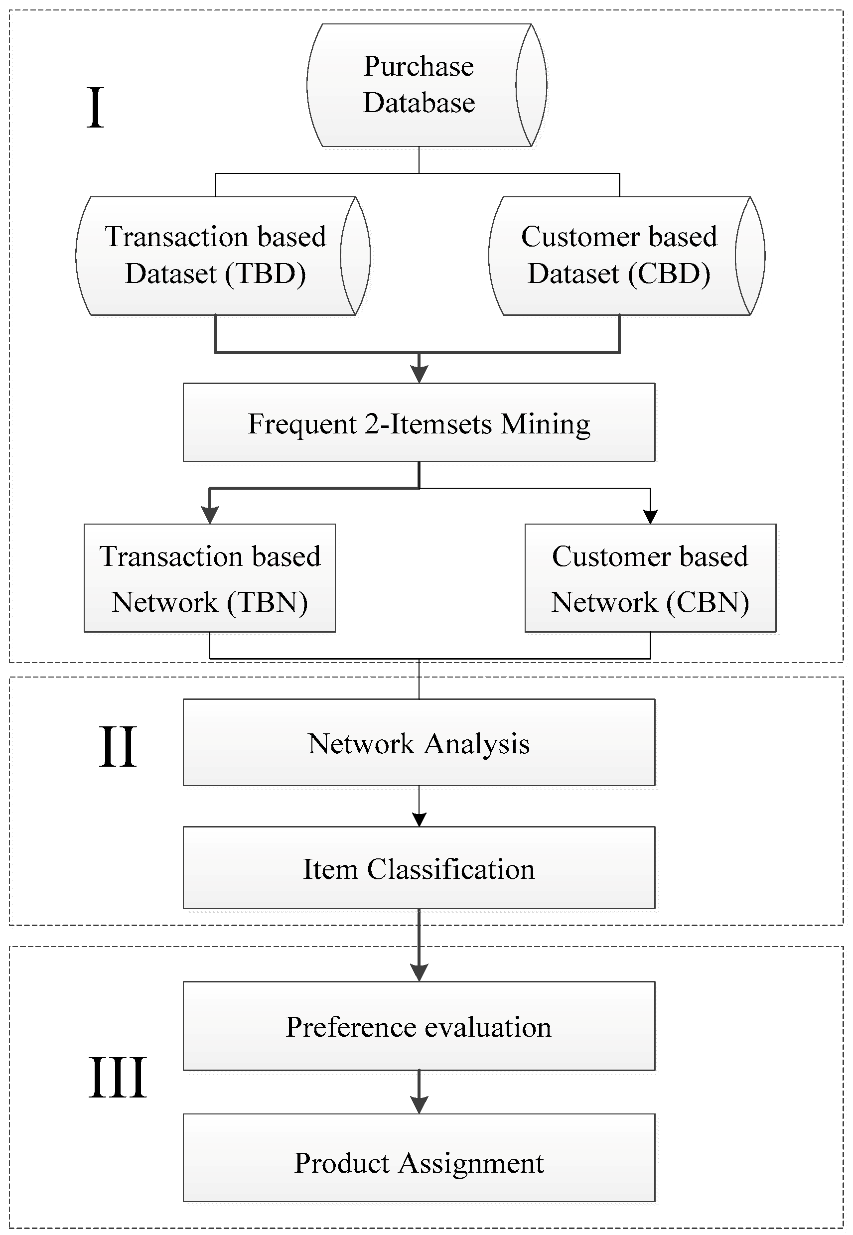
Placing products with a high degree of association close to each other raises the likelihood of cross-selling. This paper seeks to develop a method that allocates products to suitable shelves to maximize such associations and thus drive cross-selling. Figure 1 shows the proposed three-stage framework. The first stage constructs a Product Relationship Network (PRN) that represents the purchasing association among the product items. Two types of PRNs—transaction-based networks (TBN) and customer-based networks (CBNs)—are used, depending on how purchasing data are dealt with. The two PRNs will be further defined in Section 3.2. The second stage uses network analysis to derive the centrality value of each product item, which reveals the importance of the item in its network. Based on the centrality of each product, an item is classified as an attraction item, an opportunity item, or a trivial item. Opportunity items are those to be reorganized/re-shelved. The third stage uses a product assignment algorithm to determine the optimal positions/locations for opportunity items to maximize cross-selling.

The product-to-shelf assignment problem is strongly influenced by a large number of variables that are context specific. Therefore, the following assumptions are made in this study. First, although the type of stores discussed in this study is limited, it is assumed that product volumes are identical and can be smoothly exchanged across the shelves. Second, variables such as the bargaining power of the producers, and setup cost of moving product items are not discussed in this study.

3.2. Product Relationship Networks

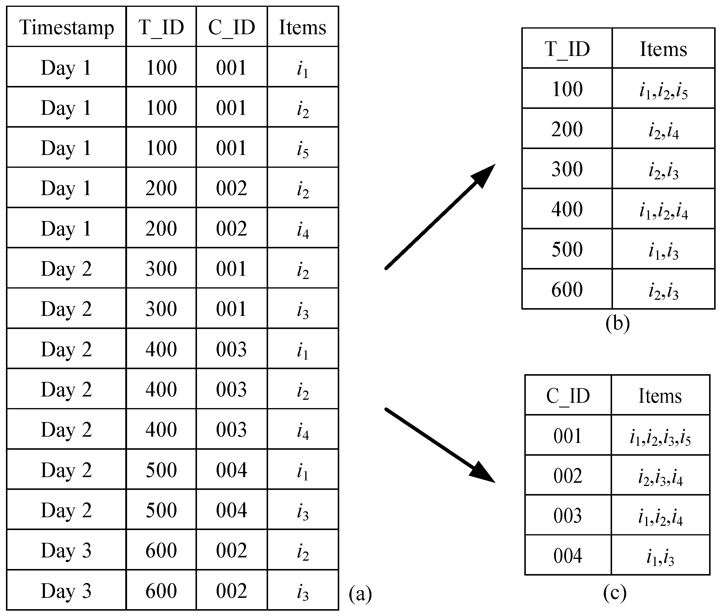
Let I = {i₁, i₂, …, i_P} be the set of product items sold in a store where P is the total number of product items. A purchase database stores a set of purchase records in which a record consists of a purchase timestamp, a transaction identifier (T_ID), a customer identifier (C_ID), and a product item. Depending on how the product relationship is constructed, product items in the purchase database can be aggregated according to unique T_ID or C_ID. If records are aggregated using T_ID, the dataset is called a transaction-based dataset (TBD). If records are aggregated using C_ID, the dataset is called a customer-based dataset (CBD). Figure 2 shows a simple aggregation example. Figure 2a indicates 14 purchase records in a purchase database. After aggregating by T_ID, 6 transaction-based records are generated as shown in Figure 2b. Similarly, as shown in Figure 2c, 4 customer-based records are generated if C_ID is used to aggregate the purchase database.

Based on different datasets, two types of Product Relationship Networks (PRNs) are constructed. If the network is constructed using the transaction-based dataset (TBD), the network is called a transaction-based network (TBN). If the network is constructed using the customer-based dataset (CBD), the network is called a customer-based network (CBN). The construction process for both types of PRNs includes the following two phases. The first phase derives all frequent 2-itemsets from an aggregated dataset using the Apriori algorithm under a minimum support count. The second phase builds the product association matrix according to the support values of frequent 2-itemsets.

The Apriori algorithm proposed by Agrawal and Srikant [7] is a popular method for identifying frequent itemsets. Let L_k represent the set of all frequent k-itemsets and C_k represents the set of candidate k-itemsets. k-itemsets may or may not be frequent, but all of the frequent k-itemsets are included in C_k. The Apriori algorithm scans the dataset and calculates the count of each candidate in C_k to determine which k-itemsets are frequent. All candidates with a count exceeding the minimum support count are frequent and belong to L_k. Otherwise, the candidates are removed. (k + 1)-itemsets of C_k+1, which include frequent k-itemsets, can be repeatedly generated by L_k. The algorithm will stop when L_k = Ø. Note that this algorithm will stop when k = 2 since only frequent 2-itemsets are required in this study.

After obtaining frequent 2-itemsets, the product association matrix of a PRN can be determined. Let M = [m_i,j] be the product association matrix of size y × y where y is the number of individual items which have ever appeared in the frequent 2-itemsets, and m_i,j is defined as:

$$m_{i,j}=SupCount(\{t_i,t_j\})$$

(1)

where SupCount is the function returning the support count of itemset {i_i, i_j}. If m_ij is high, the association between items i_i and i_j is strong. Note that if itemset {i_i, i_j} cannot be found in the frequent 2-itemsets, the support count m_i,j will be marked as “x” in the matrix.

In TBN, records with the same transaction ID are aggregated so that the association value between two items indicates the co-purchase relationship from the viewpoint of transactions. In CBN, records with the same customer ID are aggregated so that the association between items in CBN indicates the co-purchasing relationship from the viewpoint of customers. That is, CBN treats each customer in the store as equally important, while TBN might favor frequent buyers.

3.3. Network Analysis for Item Classification

After the product association matrix is obtained, a product item is considered to be a node in a network where a link between two nodes indicates their association strength. In the network, the centrality measure is used to determine the importance of each product item in the store. With this importance, each product is classified as an attraction item, an opportunity item, or a trivial item. Opportunity items are those to be reorganized/re-shelved in the third stage.

3.3.1. Network Analysis

Centrality measure is a popular index used to identify the relative importance of nodes in the network; a higher value indicates the node has a stronger effect in the network. This research uses the two most popular centrality measures, closeness and betweenness [28]. Closeness centrality measures how close a node is to all other nodes. A node is considered to be central if it can reach all others quickly. Formally, closeness centrality C_c(i) is the reciprocal of the sum of the shortest distance from node i to each other node, which can be formulated as:

$$C_C(i)=\frac{1}{{\displaystyle \sum {}_{j=1}^{N}d(i,j)}}$$

(2)

where d(i, j) is the distance of the shortest path from node i to node j in the network, and N is the total number of nodes in the network.

Betweenness centrality is a measure of centrality in a network based on shortest paths. For every pair of nodes in a network, there exists at least one shortest path between the nodes such that either the number of edges that the path passes through (for unweighted graphs) or the sum of the weights of the edges (for weighted graphs) is minimized. The betweenness centrality for node i, C_B(i), is the number of these shortest paths that pass through node i. Mathematically, it is defined as:

$$C_B(i)={\displaystyle \sum _{i\ne s}^N{\displaystyle \sum _{i\ne t}^N\frac{g_{s,t}(i)}{g_{s,t}}}}$$

(3)

where g_s,t is the number of shortest paths from node s to node t and g_s,t(i) is the number of the shortest paths from node s to node t that pass through node i. In this study, the Dijkstra algorithm [29] is used to find the shortest path between two nodes.

3.3.2. Item Classification

As mentioned in Section 1, not all items are suitable for rearrangement since established shopping behaviors might be disrupted if major attractive items are relocated. To determine item suitability for relocation, this study classifies each product item as an attraction item, an opportunity item, or a trivial item based on its centrality measure.

Definition 1.

An attraction item is an item whose centrality value is higher than an upper bound threshold value α in PRN. Attraction items should not be relocated because doing so would disrupt their connection to other products. In the following discussion, the set of attraction items is denoted as$AI=\left\{i_j\right|C(j)>\alpha \}$where C(j) is the centrality for item i_j.

Definition 2.

An opportunity item is an item whose centrality value is no greater than α but higher than a lower bound threshold value β in PRN. Opportunity items are commodities affiliated with attraction items and might sell better if moved to a more appropriate section/shelf. Therefore, opportunity items are considered to be commodities which should be re-allocated. The set of opportunity items is denoted as$OI=\left\{i_j\right|\alpha \ge C(j)>\beta \}$.

Definition 3.

A trivial item is an item whose centrality value is no greater than β. Trivial items are items which do not show a strong association with other items in PRN. Thus reallocating trivial items might not generate additional sales. The set of trivial items is denoted as$TI=\left\{i_j\right|\beta \ge C(j)\}$.

3.4. Location Preference Evaluation

As mentioned in Section 3.3.2, opportunity items are those that are re-organized, while attraction items and trivial items are kept in their original locations. To maximize cross-selling, an opportunity item should be moved to a cell close to that of its related attraction items. For example, bottle openers should be placed near bottled beers instead of canned beers. Therefore, the location preference for opportunity items will be evaluated according to purchase association and physical proximity.

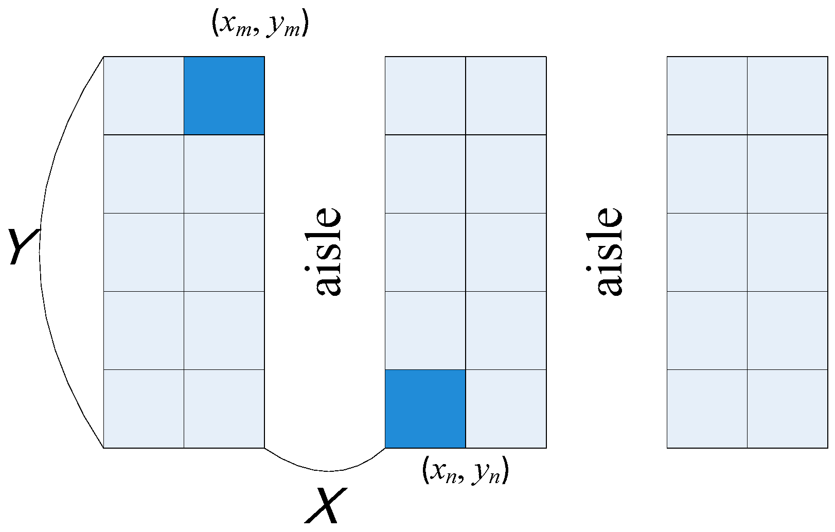
Figure 3 illustrates a typical layout consisting of cabinets and aisles in a retail store. A cabinet consists of several cells where a cell is a space used to display a product item. Let (x_m, y_m) and (x_n, y_n) respectively be the center coordinates of cell m and cell n. The physical distance between the two cells is defined as:

$$g_{m,n}=\{\begin{array}{ll}\left|x_m-x_n\right|+\left|y_m-y_n\right|& \mathrm{if}{A}_m=A_n\\ \left|x_m-x_n\right|+\min \left[(2Y-y_m-y_n),(y_m+y_n)\right]& \mathrm{if}{A}_m\ne A_n\end{array}$$

(4)

where A_m is the aisle number of cell m, A_n is the aisle number of cell n, and Y is the length of a cabinet. Based on Equation (4), we can derive a physical distance matrix G = [g_m,n] that shows the physical relationship among all cells.

It is clear that an opportunity item i_i should be placed in a cell close to the set of attraction items, AI. In addition, if the purchase association between the attraction item i_j and the opportunity item i_i is stronger, items i_j and i_i should be placed closer together. Thus, location preference in which opportunity item i_i is placed to cell m is defined as:

$$l_{i,m}={\displaystyle \sum _{j\in AI}{p}_{i,j}\times g_{m,Cell(j)}}\mathrm{for}\mathrm{all}m\in Cell(k)\mathrm{where}k\in OI$$

(5)

where p_i,j is the support count for itemset {i_i, i_j} defined in Equation (1), g_m,Cell(j) is the physical distance between cells m and Cell(j), and Cell(j) is the function returning the cell to which item i_j belongs.

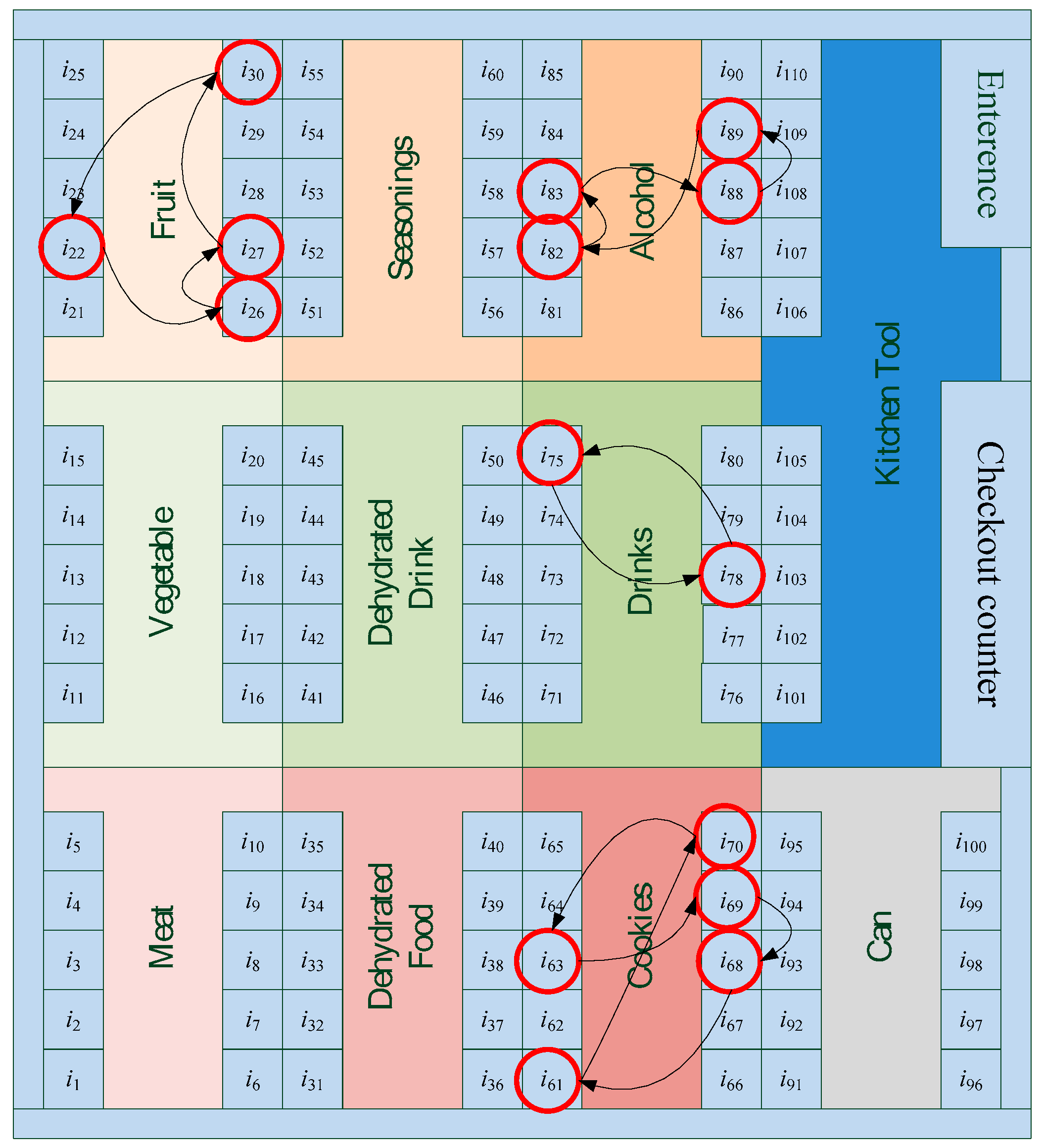
Product items belong to specific product categories such as beverages, snacks, or fresh food. For management purposes and shopping convenience, a store layout is divided into many zones, each of which is devoted to a single product category. Therefore, the cells to which opportunity items can be moved should be limited by management constraints. Let a_i,m be the likelihood availability that opportunity item i_i is placed in cell m:

$$a_{i,m}=\{\begin{array}{l}1\mathrm{if}\mathrm{item}{i}_i\mathrm{is}\mathrm{allowed}\mathrm{to}\mathrm{be}\mathrm{placed}\mathrm{on}\mathrm{cell}m\\ 0\mathrm{if}\mathrm{item}{i}_i\mathrm{cannot}\mathrm{be}\mathrm{placed}\mathrm{on}\mathrm{cell}m\end{array}$$

(6)

Finally, the final location preference lp_i,m can be derived as:

$$l{p}_{i,m}=l_{i,m}\times a_{i,m}$$

(7)

3.5. Product Assignment

This research assumes that all product items have identical sizes and quantities so that two opportunity items on different shelves can be easily exchanged. The reassignment considers the location preference defined in Equation (7) and reassigns products to the most suitable shelves. Therefore, the objective of product rearrangement is to rearrange opportunity items while minimizing total shelf movement:

$$MIN{\displaystyle \sum _{i=1}^{\left|OI\right|}{\displaystyle \sum _{j=1}^{\left|OI\right|}(E_{i,j}\cdot l{p}_{i,Cell(j)})}}$$

(8)

subject to:

$$\begin{array}{c}{\displaystyle \sum _{j=1}^{\left|OI\right|}{E}_{ij}=1,i=1,2,\dots ,}\left|OI\right|\\ {\displaystyle \sum _{i=1}^{\left|OI\right|}{E}_{ij}=1,j=1,2,\dots ,}\left|OI\right|\\ E_{ij}\ge 0foralliandj\end{array}$$

where opportunity items i and j ∈ OI, E_ij = 1 if opportunity item i is assigned to a shelf which displays opportunity item j, otherwise E_ij = 0. The item assignment problem shown in Equation (8) is solved using the Hungarian method [30], a combinatorial optimization algorithm that can solve the assignment problem in polynomial time. Appendix A shows the computational procedure of the Hungarian method.

4. Implementation and Experimental Results

In this section, a case study is conducted to show the benefits and strengths of the proposed three-stage product-to-shelf assignment method. In Section 4.1, the data and case study environment are introduced. Then, a set of experiments for the case study are illustrated in Section 4.2. Finally, sensitive analysis is described in Section 4.3.

4.1. Environment and Data Description

Figure 4 illustrates the layout of a simplified grocery store to demonstrate the feasibility of the proposed shelf space allocation method. There are 110 product items in the store, with each product item belonging to one of 11 categories such as meat, vegetable, fruit, dried food, etc. Products are assigned to a specific zone according to their category. The initial position (location) assignment for products and center coordinates of cells are respectively shown in Figure 4a,b.

A transaction generator is developed to simulate customer shopping behavior. In this generator, four types of customers are modeled. Each with different purchasing probabilities for the various product categories (

Table 1. Four customer types and their purchase behavior.

Customer Type	Purchase Probability for All Categories
Type I	Meat (10%), Vegetable (10%), Fruit (10%), Dehydrated Food (10%), Dehydrated Drink (10%), Seasonings (10%), Cookie (10%), Drink (10%), Alcohol (10%), Can (5%), Kitchen Tool (5%)
Type II	Fruit (16%), Dehydrated Food (16%), Dehydrated Drink (8%), Cookie (8%), Drink (8%), Alcohol (16%), Can (8%), Meat (30%), Vegetable (30%), Seasonings (30%), Kitchen Tool (10%)
Type III	Dehydrated Food (20%), Dehydrated Drink (20%), Cookie (20%), Drink (20%), Meat (5%), Vegetable (5%), Fruit (4%), Seasonings (3%), Can (2%), Kitchen Tool (1%)
Type IV	Alcohol (40%), Kitchen Tool (40%), Meat (2%), Vegetable (2%), Fruit (4%), Dehydrated Food (1%), Dehydrated Drink (2%), Seasonings (1%), Cookie (3%), Drink (3%), Can (3%)

), and are assigned different weightings for transaction frequency (respectively 60%, 20%, 15%, and 5%). In this study, the total number of purchase transactions in the generator is set at 5000.

Table 2. Simulated purchase dataset.

T_ID	C_ID	Product Item
1	A02577	i16, i32, i37, i42, i55, i61, i71, i77
2	A06359	i16, i74, i86
3	A11223	i15, i89, i97, i99
…	…	…
4998	A60825	i86
4999	A69390	i9, i10, i56, i86, i108
5000	A71889	i8, i15, i27, i28, i59, i91, i98

summarizes part of the simulated purchase transactions where a transaction contains T_ID (transaction identifier), C_ID (customer identifier), and purchased product items. Next, the purchase dataset will be respectively aggregated as a transaction-based dataset (TBD) and a customer-based dataset (CBD) according to unique T_ID or C_ID. After this process, the number of records in TBD is 5000 while the number of records in CBD is 1000.

4.2. A Case Illustration

Based on the different datasets, two types of Product Relationship Networks (PRN) are constructed. A network based on the transaction-based dataset (TBD) is called a transaction-based network (TBN), while one based on the customer-based dataset (CBD) is called a customer-based network (CBN). For the sake of simplicity, only the CBN experiment is reported in this section, and the performance of TBN and CBN will be compared in Section 4.3. When the minimum support count in the Apriori algorithm is set to 50, the product association matrix for CBN can be generated. Based on the matrix, the connection among all products in CBN is visualized in Figure 5. Note that the product item name is shown in the graph instead of the product item number.

Based on the matrix, the closeness centrality and betweenness centrality for all products in CBN can be evaluated using Equations (2) and (3). Next, each product item is classified as an attraction item, an opportunity item, or a trivial item according to Definitions 1 to 3. When α = 10 and β = 5, there are 29 attraction items, 26 opportunity items, and 55 trivial items for CBN.

Table 3. Item classification example.

Type	Item	Betweenness Value
Attraction Item (29)	i45	278.131
	i31	75.547
	i33	75.547
	…	…
	i87	10.602
	i28	10.082
Opportunity Item (26)	i75	8.671
	i78	8.671
	i27	8.671
	…	…
	i73	5.225
	i47	5.157
Trivial Item (55)	i90	4.921
	i19	4.485
	i62	4.196
	…	…
	i91	0
	i110	0

shows the classification result for CBN.

Next, the location preference can be calculated using Equations (4)–(7). Based on the location preference values, the Hungarian method is used to solve the assignment problem.

Table 4. Reassignment result for 15 opportunity items for CBN.

Items	Original Cell	New Cell	Items	Original Cell	New Cell
i22	C22	C26	i70	C70	C63
i26	C26	C27	i75	C75	C78
i27	C27	C30	i78	C78	C75
i30	C30	C22	i82	C82	C83
i61	C61	C70	i83	C83	C88
i63	C63	C69	i88	C88	C89
i68	C68	C61	i89	C89	C82
i69	C69	C68

shows the reassignment result for CBN using betweenness centrality. Among 26 opportunity items, the locations of 15 items (i₂₂, i₂₆, i₂₇, i₃₀, i₆₁, i₆₃, i₆₈, i₆₉, i₇₀, i₇₅, i₇₈, i₈₂, i₈₃, i₈₈, i₈₉) will be exchanged and the locations of 11 items (i₃, i₁₃, i₁₅, i₂₃, i₂₄, i₄₁, i₄₃, i₄₇, i₆₅, i₇₂, i₇₃) will stay the same. For example, item i₆₃ will be moved from its original cell (C₆₃) to the new cell (C₆₉), while item i₃ will stay in its place. Figure 6 shows the locations of the 15 opportunity items that will be re-shelved.

4.3. Sensitive Analysis

This section analyzes how parameters in our method affect the final reassignment result.

4.3.1. Analysis of Minimum Support Count

When constructing a Product Relationship Network (PRN), the minimum support count in the Apriori algorithm is an important threshold since it is used to remove the links between nodes with weak association values. A high threshold value produces a network with few links. However, determining an appropriate minimum support count is a difficult task. To address this issue, the concept of “accumulated percentage of active links” is proposed to help users determine the threshold value. Note that an active link is defined as the link between two products whose association is greater than the minimum support count in the PRN.

Figure 7 shows the relationships among the settings of minimum support counts, the number of active links, and the accumulated percentage of activate links in TBN. There are 5995 possible active links among 110 products when the minimum support count is set at 0. If the minimum support count is set at 15, the accumulated percentage of active links will be 30% (= 1799/5995). That is, store managers expect that at most 30% of items (i.e., around 33 items) might be exchanged. Similarly, when the minimum support count is set at 20, the accumulated percentage of active links will be 12% (= 719/5995), which indicates that at most 12% of items (i.e., around 13 items) might be moved. Based on the information in the figure, managers can determine the appropriate minimum support count with consideration of re-shelving cost. Similarly, Figure 8 shows the relationship among the settings of minimum support count, number of active links, and accumulated percentage of activated links in CBN.

Based on the two figures, it is clear that the number of active links falls as the minimum support count increases. However, if the minimum support count is set the same for TBN and CBN, the number of active links in CBN is larger than that in TBN because most association values in the links in CBN are stronger than those in TBN. In addition, when the minimum support count is low, the centrality value will be affected by a large number of nodes with weak associations, thus reducing the significance of the reassignment result. Conversely, when the minimum support count is high, the centrality value is derived based on a smaller number of nodes with strong association, thus increasing the significance of the reassignment result.

4.3.2. Analysis of Product Relationship Networks

To understand the characteristics of TBN and CBN, we use five popular indexes: Density, isolated product, diameter, average shortest distance, and clustering coefficient [31]. Density is the number of links divided by the number of total potential links. Diameter is the maximum distance between any pair of nodes in the network. Average shortest distance is the average of all-pairs shortest distance. A clustering coefficient is a measure of the degree to which nodes in a network tend to cluster together.

Table 5. Five indexes under different minimum support count in TBN.

Minimum Support Count	Density	Isolated Product	Diameter	Average Shortest Distance	Clustering Coefficient
5	0.905	0	2	1.095	0.936
10	0.621	0	3	1.389	0.856
15	0.382	12	4	1.632	0.656
20	0.124	29	4	1.936	0.491
25	0.034	48	6	2.541	0.228
30	0.007	80	7	2.762	0.153

shows the values of the five indexes when minimum support count is 5, 10, 15, 20, 25, and 30 for TBN.

Table 6. Five indexes under different minimum support count in CBN.

Minimum Support Count	Density	Isolated Product	Diameter	Average Shortest Distance	Clustering Coefficient
30	0.827	0	2	1.173	0.974
40	0.707	3	3	1.257	0.951
50	0.579	13	3	1.258	0.911
60	0.374	20	3	1.445	0.829
70	0.211	30	3	1.62	0.801
80	0.118	47	5	1.886	0.767

shows the values of the five indexes when minimum support count is 30, 40, 50, 60, 70, and 80 for CBN.

According to Table 5 and Table 6, when the minimum support count is high, the density of the two product networks will be low since there are few active links in the product network. The network density of the two networks is similar when the minimum support count is 15 in TBN and 60 in CBN. However, the number of isolated nodes in CBN is much higher than in TBN since CBN aggregates customer transactions. Similarly, the average shortest distance and diameter in CBN is shorter than in TBN.

It is clear that the product associations derived from TBN are based on individual transactions. That is, TBN considers each transaction to be equally important so that repeated purchases will be accumulated/counted when conducting association analysis. This makes TBN suitable for stores with fewer customers with higher loyalty. On the other hand, the product associations derived from CBN are based on individual customers. The analysis result derived from CBN will be less affected by customers who repeatedly purchase the same products. Therefore, CBN is suitable for stores with large numbers of one-time customers.

4.3.3. Analysis of Attraction and Opportunity Items

In this research, a product item is classified as attraction item, opportunity item, or trivial item based on its centrality measure and parameters of α and β. An item whose centrality value is higher than α is called an attraction item. An item whose centrality value is between α and β is called an opportunity item. Otherwise, an item is a trivial item. Figure 9 shows the relationship between the number of attraction items and threshold value α in TBN using betweenness centrality. If α is greater than 50, the number of attraction items will not exceed 12, which might be too few for location preference evaluation. Therefore, α < 50 is suggested in this experiment when betweenness centrality is adopted.

Table 7. Number of attraction and opportunity items using betweenness centrality.

α	β	Number of Attraction Items	Number of Opportunity Items
30	10	28	37
30	15	28	25
30	20	28	18
40	10	19	46
40	15	19	34
40	20	19	27
50	10	12	53
50	15	12	41
50	20	12	34

shows the possible outcomes when changing parameters α and β.

Figure 10 shows the relationship between the number of attraction items and the threshold value α in TBN using closeness centrality. If α exceeds 170, the number of attraction items will not exceed 20, which might be too few for location preference evaluation. Therefore, α < 170 is suggested in this experiment when betweenness centrality is adopted.

Table 8. Number of attraction and opportunity items using closeness centrality.

α	β	Number of Attraction Items	Number of Opportunity Items
150	135	34	29
150	140	34	9
150	145	34	5
160	135	24	39
160	140	24	25
160	145	24	15
170	135	20	43
170	140	20	29
170	145	20	19

shows the possible outcomes when changing parameters α and β.

Attraction items bring customers into the store. Thus the number of attraction items should be maximized and their locations should remain consistent. By contrast, opportunity items should be moved to maximize cross-selling. Reassignment of a large number of opportunity items will entail considerable labor and expense, but limiting the number of opportunity items to be reassigned may limit the impact on purchasing.

5. Discussion and Conclusions

To attract customers and survive in a competitive environment, retailers need to implement appropriate retail-mix strategies including store location, product assortment, pricing, advertising and promotion, store design and shelf display, services, and personal selling. Among these, shelf-space allocation is one of the most important factors in determining customer purchasing decisions. Recently, advances in information technology have made it easier for retailers to collect various types of customer data. Mining this data for insight into customer behavior can help retailers solidify ephemeral relationships with customers into long-term loyalty. As part of this effort, retailers have modified their shelf-space management practices using product association analysis. Previous studies have demonstrated that product association analysis can improve the efficiency of shelf space usage and increase cross-selling.

This study solves the persistent product-to-shelf allocation problem by integrating data mining and network analysis, and makes three major contributions. First, the study compares the effectiveness of transaction-based networks (TBN) and customer-based networks (CBN). Experimental results show that the two network types produce very different association values among products. If store managers want to reduce side effects caused by customers repeatedly purchasing the same products, CBN is a better choice than TBN. Conversely, TBN is more useful if store managers treat all transactions as equally important. Second, this research uses network analysis to evaluate product centrality, and uses the resulting centrality value to classify products as attraction items, opportunity items, or trivial items. Attraction items are popular products which attract customer visits, and should be kept in consistent locations making them easy to find. On the other hand, opportunity items should be relocated to increase cross-selling. Third, this study considers product association along with physical proximity and category constraints when solving the product-to-shelf assignment problem.

Some potential extensions for this research are as follows. First, the proposed method uses closeness and betweenness to measure product centrality in the product relationship network. Different centrality measures give different meanings and future studies should apply a wider range of centrality measures. Second, this study assumes product volumes are identical and can be smoothly exchanged. However, in practice, different products might be displayed in different volumes, and future work should consider this issue. Third, some additional limitations that could be addressed are those concerning restrictions on storage conditions of certain products (e.g. frozen or refrigerated products) or consideration of product relocation costs. Meanwhile, it would be interesting to take the height of positioning within a shelf into consideration. Fourth, this study solves the product-to-shelf assignment using the Hungarian method, which would run too slowly given large quantities of data. Finally, the proposed method is now validated and evaluated using simulated behavior data produced by a transaction sequence generator, and future work should apply authentic store transaction data.