Cultivar Classification of Single Sweet Corn Seed Using Fourier Transform Near-Infrared Spectroscopy Combined with Discriminant Analysis

Abstract

Seed purity is a key indicator of crop seed quality. The conventional methods for cultivar identification are time-consuming, expensive, and destructive. Fourier transform near-infrared (FT-NIR) spectroscopy combined with discriminant analyses, was studied as a rapid and nondestructive technique to classify the cultivars of sweet corn seeds. Spectra with a range of 1000–2500 nm collected from 760 seeds of two cultivars were used for the discriminant analyses. Thereafter, 126 feature wavelengths were identified from 1557 wavelengths using a genetic algorithm (GA) to build simplified classification models. Four classification algorithms, namely K-nearest neighbor (KNN), soft independent method of class analogy (SIMCA), partial least-squares discriminant analysis (PLS-DA), and support vector machine discriminant analysis (SVM-DA) were tested on full-range wavelengths and feature wavelengths, respectively. With the full-range wavelengths, all four algorithms achieved a high classification accuracy range from 97.56% to 99.59%, and the SVM-DA worked better than other models. From the feature wavelengths, no significant decline in accuracies was observed in most of the models and a high accuracy of 99.19% was still obtained by the PLS-DA model. This study demonstrated that using the FT-NIR technique with discriminant analyses could be a feasible way to classify sweet corn seed cultivars and the proper classification model could be embedded in seed sorting machinery to select high-purity seeds.

1. Introduction

The sweetness of sweet corn is a major factor in consumer satisfaction, which attracts a high interest from breeders to breed sweeter corn cultivars [1]. Unlike most other crops, sweet corn is mainly consumed when it is immature because of its nutrition and sweet flavor [2]. Some characteristic genes of sweet corn cultivars, such as sugary-1, sugary enhanced, and shrunken, can make the conversion of sugar to starch negligible before the kernels fully ripen [3]. For this reason, a uniform maturity time is crucial for farmers to choose the optimal harvest time, and then to obtain a proper shelf-life quality as the sweet flavor of sweet corn changes quickly after harvesting [4]. However, different cultivars of sweet corn will vary in the maturity cycle, even under the same planting conditions [5]. Hence, it is significant to develop methods for distinguishing the cultivars of sweet corn seeds and making the maturity time consistent. The purity of a seed cultivar is defined as the ratio of seeds belonging to a cultivar to the total tested seeds [6]. After removing other cultivars of sweet corn seeds, the tidy harvest time can be obtained with the pure cultivar seeds. Moreover, because the economic value, nutritional value, and resistance to diseases and pests of sweet corn are also related to the cultivar attributes [7], improving the purity of sweet corn seed can also ensure the quality and yield [8], and eventually increase the economic benefits of agricultural production. Consequently, detecting the purity of seed cultivars is necessary before sowing to avoid different cultivars of seeds being mixed during the production process, such as cultivation, harvesting, transportation, and storage procedures [6].

Morphology identification, physiochemistry analysis, and molecular identification are three types of conventional methods that may be used to identify sweet corn cultivars. These methods, including protein electrophoresis and DNA molecular markers, are time-consuming, costly, and destructive [9]. Thus, these methods may be used to detect a small group of sampling seeds. The complex sample preparation required for such detection methods also limits the possibilities of using these methods for online detection in the seed industry [10]. In view of these drawbacks, researchers have shown great interest in looking for rapid and non-destructive methods for seed cultivar detection.

Hyperspectral imaging (HSI) is recognized to be a promising technique to detect seed cultivars by combining the advantages of computer vision and near-infrared spectroscopy (NIRS). It obtains spatial images of samples over a range of electromagnetic spectrums. The HSI data are generally described as a three-dimensional cube, which has two dimensions for pixel coordinates in the physical and spatial domain and one dimension for wavelengths. As previous research has reported, Zhang et al., (2012) applied an HSI system (380–1030 nm) for distinguishing varieties of maize seeds, where the highest accuracy at 98.89% was achieved by a support vector machine (SVM) algorithm [11]. Kong et al., (2013) used an HSI system (1039-1612 nm) to identify rice seed cultivars, and the prediction rates of all the tested models were over 80%, and they also reported that the performances of the optimal wavelength-based were worse than the full-range models under the experimental data [12]. Yang et al., (2015) studied the feasibility of classifying the varieties of waxy maize seeds using a customized HSI system (400–1000 nm), where they found that the spectra collected from the germ side generated a slightly higher accuracy than the spectra collected from the endosperm side [6]. Wang et al., (2016) successfully utilized an HSI (400–1000 nm) to classify different varieties of maize seeds by combining spectral data and textural features [7]. Zhao et al., (2018) succeeded in using the HSI (874–1734 nm, 975.01–1645.82 nm) with a radial basis function neural network algorithm for maize seed variety classification at an accuracy of 91.0% [13]. This HSI system was also used to discriminate the varieties of grape seed, where the highest accuracy of 88.7% was achieved in the prediction set [14]. Xie et al., (2018) carried out research to recognize the varieties of mung beans using the HSI (380–1023 nm) system, where the extreme learning machine algorithm performed with accuracies ranging from 99.17% to 100% [10]. Qiu et al., (2018) utilized two HSI systems with different spectral ranges (380–1030 nm and 874–1734 nm) to identify rice seed varieties. Three modeling methods, including the K-nearest neighbor (KNN), SVM, and convolutional neural network, were tested. They came to the conclusion that long-wave spectra (874–1734 nm) could result in a higher accuracy than that of short-wave spectra (380–1030 nm) among three modeling methods [15]. This research demonstrated that spectral features identified by HSI are useful for cultivar classification. However, the HSI technique used in the above research can only show the features in the short-wave spectral range. All these HSI systems had a spectral range no greater than 1750 nm because of the limited capability of the detector sensor in the HSI system. The spectral range above 1750 nm may include more information and should also be studied to optimize cultivar classification.

The Fourier transform near-infrared (FT-NIR) technique is an emerging method that can easily measure spectral responses in a wide wavelength range of near-infrared (NIR). The FT-NIR technique is also characterized by high-resolution and accurate frequency determination. It has been widely studied in seed quality detection because of its advantages of a high speed and low cost, and its non-contact detection features give it considerable potential for online detection. Thus far, FT-NIR spectroscopy has been studied in detecting the composition contents [16,17,18], viability [19,20,21,22,23], and contaminations [24,25,26] in various varieties of grains or seeds. Attaviroj et al., (2011) applied FT-NIR spectroscopy to classify five varieties of rice and achieved a high accuracy of 99.22% using the partial least-squares discriminant analysis (PLS-DA) modeling method [27]. Chen et al., (2016) showed that a reasonable accuracy can be obtained while using Fourier transform mid-infrared (FT-MIR) and FT-NIR spectroscopy to classify species of sorghum seeds [28]. Cui el at. (2018) established models based on FT-NIR data to identify maize varieties, and they obtained an average accuracy greater than 90% [9]. However, most of the studies could achieve applicable results using a batch of seeds as a sample. It can still be a challenge to measure the spectrum of single seeds for cultivar detection, especially when the contents of compositions inside the seed samples are highly similar.

This study was carried out to classify two similar sweet corn seed cultivars using FT-NIR spectroscopy, with a wavelength range of 1000–2500 nm. It was aimed at developing a rapid, economical, and non-destructive method for ensuring the purity of seeds. The GA method was used to identify feature wavelengths to simplify the discriminant models. Given that previous studies [11,15] have shown that different modeling methods may achieve unequal accuracies, four classification algorithms, namely KNN, the soft independent method of class analogy (SIMCA), PLS-DA, and support vector machine discriminant analysis (SVM-DA), were tested on the full-range and feature wavelengths to obtain the optimal classification model. Three validation methods, namely, cross-validation, the independent test, and the permutation test, were applied for optimizing and validating the reliabilities of all models. The performances of all models were compared and discussed in this study.

2. Materials and Methods

2.1. Seed Samples

In this study, a total of 760 seed kernels were randomly selected from two sweet corn cultivars as experimental materials: 380 from cultivar Huameitian No.8 (H8) and another 380 from cultivar Huameitian No.168 (H168). These two cultivars have similarity and difference in breeding parents. On one hand, the H8 and H168 cultivars were bred from the same male parent, code-named H068. On the other hand, their female parents were different. For the cultivar H8, its female parent was bred from the sweet corn cultivar 03AX-538BC, which originated from the USA. For the cultivar H168, its female parent was bred from another sweet corn cultivar ACX232, which also originated from the USA. Because there was a transmission of genetic information between the parents and their offspring, both of these two sweet corn cultivars could obtain a high sugar content in fresh stages. The soluble sugar content in cultivar H168 can reach 30.47% (from 24.86% to 30.47%), which is slightly higher than that in the cultivar H8 (from 21.12% to 22.09%) [29,30]. However, the morphological characteristics were similar among these two cultivars, and it was difficult to observe visual differences between these two cultivars.

2.2. FT-NIR Spectroscopy Acquisition

To investigate the feasibility of distinguishing the cultivars of sweet corn seeds at a single-kernel level, the FT-NIR spectra of all 380 sweet corn seeds in each cultivar were collected using a Fourier transform infrared spectrometer (Antaris II FT-NIR Analyzer; Thermo Scientific Co., Waltham, MA, USA). The supporting control software of the spectrometer (RESULT, Thermo Scientific Co., Waltham, MA, USA) was used to set the instrument parameters and record the spectra. Figure 1 shows the schematic of the FT-NIR spectroscopy acquisition for sweet corn seed kernels. The spectrometer used an InGaAs detector with a high sensitivity and stability to NIR signals and a high-intensity halogen light as the light source. It also used an integrating sphere in a diffuse reflectance mode to improve the spectral quality of heterogeneous samples. The seed kernel was placed in a cylindrical sample cup with a diameter of 10 mm. The cup had a quartz window on the bottom, through which the light source irradiated the seed sample. Because of the difference of the structure and composition between the two sides of the corn seed and the limited penetration depth of the light source, the pre-experiment showed that the spectra collected from the embryo side and endosperm side were significantly different. While using the Euclidean distances and spectral angles as the evaluation index to evaluate the difference between spectrums, the differences between the mean spectrums from two sides of kernels within the same cultivar were in the same order of magnitude as those of two cultivars from the same embryo side. Hence, only the spectra that were collected while the light source irradiated the embryo side of the seeds were used in this study. The spectra were collected at a resolution of 4 cm⁻¹ intervals (0.6 nm at 1250 nm), crossing the range of 10,000 to 4,000 cm⁻¹ (1000–2500 nm), containing 1557 wavelength points per spectrum. The mean spectrum from 32 successive scans of each individual seed was used as the seed spectrum. Finally, 760 spectra in total were obtained and stored as log$\left(1/R\right)$, where $R$ is the relative reflectance signal value corrected by the supporting control software with the white and dark reference using the following equation:

$$R= \frac{R_0 - D}{W - D}$$

(1)

where $R_0$ was the original reflectance intensity in each wavelength from the seed samples, $W$ was the reflectance intensity from the internal gold reference flag when the light source was turning on, and $D$ was the reflectance intensity from the internal gold reference flag when the light source was turning off.

To minimize the effects of temperature and moisture fluctuations during spectral acquisition [31], the spectrometer instrument was fully preheated and placed in an environment with a temperature of 25$\pm$1 °C and a relative humidity of 50$\pm$3%. The seed samples were also placed in the same environment for more than 30 days before the collection of the spectra.

2.3. Data Pre-processing

The spectra of all the samples combined with cultivar names were imported and organized as a dataset file. MATLAB (MathWorks, Natick, MA, USA) with the PLS Toolbox v.8.2.1 function (Eigenvector Research Inc., Wenatchee, WA, USA) was utilized for handling the dataset and calibrating the discriminant models.

A robust model performance relies on high-quality data. Outliers in the calibration data set may result in low accuracy models [32]. Therefore, outlier detection is necessary before calibrating discriminant models. Principal component analysis (PCA) was applied to detect outliers of the spectra by examining the Q Residuals and Hotelling’s T². The Q Residuals calculated from the PCA model were the measure of the difference between an original spectrum and its PCA projection. The Hotelling’s T² value was another parameter indicating how far a spectrum was away from the projection center (PCA scores are zeros) in the principal components’ (PCs) space. A spectrum with a high Q Residual or a high Hotelling’s T² could be treated as an outlier sample with a reasonable possibility [33]. In this study, spectral vectors of each cultivar were subjected to the PCA process for outlier detection. The statistics Q Residual and Hotelling’s T² were calculated while using the first three PCs model. Samples were marked as outliers when their Q Residual or Hotelling’s T² value exceeded the confidence interval at a 99% confidence level.

After removing the outliers and regularizing the spectra, the remaining samples in each cultivar were divided into two parts. One-third of them were selected at equal intervals as an independent testing set, and the remaining two-thirds were used as the training set for calibrating models.

Appropriate pre-processing methods may improve model accuracy by removing systemic noise and normalizing the data. The smoothing method was commonly used to reduce high-frequency noise. All the full-range spectral data were pre-processed with the Savitzky–Golay filter, using a 21-point-window and third-order polynomial [21]. Scattering theory states that scattering should have an additive and/or a multiplicative effect on reflection spectra caused by optical path-length variations and particle size uniformity, and these features generally had a negative impact on the calibration model development. The scattering profile in a spectrum can be deduced from the ideal standard spectrum. Multiplicative scatters correction (MSC) was developed to reduce the effect of scattered light on reflection NIR spectra [34]. This study used the mean spectrum of the training set as the standard spectrum when processing MSC. The MSC method determined the scattering by regressing each spectrum onto the mean spectrum, and the scatter-corrected spectrum was then calculated inversely based on the regression coefficients from the original spectrum. The spectral matrix of the full-range wavelengths was pre-processed with MSC prior to performing the discriminant analyses. Moreover, the first derivative of the Savitzky–Golay pre-processing was also applied to inspect the difference between the spectra of the two cultivars, since it could remove the predominant background variation from the spectral data.

The spectra angle which is calculated from two spectral vectors is commonly used to measure the similarities between spectrums. It can also be used as a classification technique that assigns categories to samples based on their spectral angle between the sample spectrum and reference spectrum. Hence, spectral angles were calculated to illustrate the similarities of the spectra between two cultivars and how these spectral angles change along with different pre-processing methods by the following formula:

$$\alpha = {\cos }^{-1}\frac{{{\displaystyle \sum }}_{i=1}^k{y}_i{r}_i}{\sqrt{{{\displaystyle \sum }}_{i=1}^k{y}_i^2}\sqrt{{{\displaystyle \sum }}_{i=1}^k{r}_i^2}}$$

(2)

Here, $\alpha$ was the spectral angle between the mean spectra of two cultivars, $k$ was the number of wavelength variables in a spectrum, $y_i$ was the $i^{th}$ variable value in the sample spectrum, and $r_i$ was the $i^{th}$ variable value in the reference spectrum. In this study, the mean spectrum of one cultivar was used as the reference spectrum, so the samples inside this cultivar should then have resulted in smaller spectral angle values than the samples outside the cultivar.

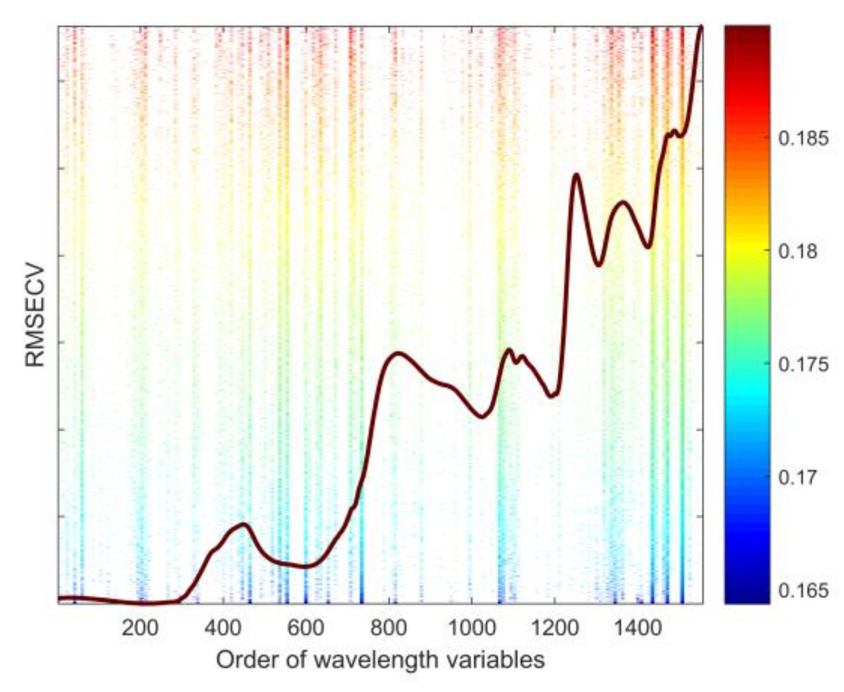
2.4. Feature Wavelengths Selection

Applying appropriate methods to select feature wavelengths for modeling would obtain the same performance as the full-range wavelength models in seed quality detection [23,35]. In this study, the genetic algorithm (GA) was utilized to identify the feature wavelengths. The GA method randomly generated sufficient subsets (each subset was called an individual), including various combinations of variables (where the variables were equivalent to the concept of genes). Since the adjacent variables contained correlated information, every nine adjacent variables were merged into one gene to improve the signal-to-noise and the speed of variable selections while performing a GA procedure [36]. Namely, 1557 variables in a spectrum were assigned to 173 genes on average.

The variables that frequently appeared in high-performance models were considered useful for cultivar distinguishing after numbers of generations of iteration. The multiple linear regression (MLR) was used as the fitness function. The root mean square error calculated from cross-validation (RMSECV) was used to evaluate the model performance. Meanwhile, to guide the GA towards solutions only using about 10% of the total variables, a penalty mechanism was added. The final RMSECV was calculated by the following equation:

$$RMSECV=RMSEC{V}_0*\left(1+\rho *n\right)$$

(3)

where $\rho$ was the penalty factor and $n$ was the number of variables included in the individual above or below the target range. In each generation, 25% of the subsets that produced poor-quality models were eliminated. After each generation, cross-over and mutation were allowed to occur within the remaining subsets, which simulated natural evolutionary processes [37]. In this way, variables that contributed to improving the performance of the models were retained, and these variables were commonly regarded as feature wavelengths.

2.5. Discriminant Analysis Algorithms

2.5.1. K-Nearest Neighbor (KNN)

The KNN Classifier is a simple but widely used method for classification purposes. It determines the category of the unknown sample according to the categories of its K nearest samples in the training set. In this study, Euclidean distance was used as a measure of the distance, and the unknown sample was assigned to a category that got more votes from the K nearest samples by means of a vote. The different number of neighbors K were tested from 3 to 19, with a step of 2 during the cross-validation process, and the number that resulted in the highest accuracy was selected as the optimal K value for discriminating samples in the testing set.

2.5.2. Soft Independent Method of Class Analogy (SIMCA)

The basic idea of SIMCA is to build a confidence limit for each category to distinguish the samples belonging to the category from the others. In this study, the confidence limit was calculated from the PCA in the training set based on the Q Residuals or Hotelling’s T² statistics [38]. All of these PCA models were treated as sub-models involved in the SIMCA model. For each sub-model, the optimal number of PCs was expected to capture more features within its category, which contributed to distinguishing samples from other categories. The optimal number of PCs was determined by cross-validation while generating the highest classification accuracy. After all of the sub-models had been built, the possibility of an unknown sample belonging to a particular category was calculated by examining the confidence level of its Q Residuals and Hotelling’s T² statistics using the following method:

$$P_{Category}= \frac{0.5*\left(1-c\right)}{1-D}$$

(4)

where $D$ was the decision limit threshold chosen as an acceptance boundary, such that the samples on the boundary $D$ would have a 50% possibility of belonging to the category. The threshold of 0.95 was chosen as the $D$ value in this study, and $c$ was the confidence level of each unknown sample, determined from the distributions of the Q Residual and Hotelling’s T². Finally, the unknown sample was assigned to the category with the higher possibility.

2.5.3. Partial Least-squares Discriminant Analysis (PLS-DA)

PLS-DA is a classification method that was developed from the partial least-squares regression (PLSR) technique by adding a threshold to the predicted values. This method is frequently used in NIR spectroscopy analyses. PLS-DA excels at handling data with collinearity, just like the characteristics of NIR spectroscopy. Specifically, PLS-DA extracts latent variables (LVs) from the predictors ($X$) and response ($Y$) to build a linear relationship between $X$ and $Y$, explained as follows:

$$Y= XB+E$$

(5)

where $B$ was the matrix of regression coefficients of the PLS-DA model, and $E$ was the residual matrix that represents the portion of variance not explained in $X$ and $Y$. In this way, redundant variables and noise information are eliminated in the residual $E$, and the useful predictors are assigned greater weights by the regression coefficients $B$. Therefore, selecting the number of LVs was crucial to avoiding underfitting or overfitting. This study followed the principle to select an appropriate number of LVs, such that the RMSECV did not change significantly or tend to go up when adding LVs to the model. The response variable $Y$ was assigned with numbers 1 and 2 to represent the cultivars of seed samples (1 for H8 and 2 for H168). However, the predicted value in the model are hardly perfect integers 1 or 2. Hence, a Gaussian distribution of calibration results was fitted to determine a probabilistic threshold as a cut off to discriminate which cultivar the unknown sample belonged to, and more details about calculating the probabilities have been described in previous work in reference [39].

2.5.4. Support Vector Machine Discriminant Analysis (SVM-DA)

As a supervised machine learning algorithm, the SVM function can efficiently handle linear and nonlinear data for regression or classification purposes [40]. The principle of the SVM algorithm is to map the original data into higher dimensional spaces, and it optimizes a hyperplane with an appropriate margin to classify different classes. The SVM used to be designed as a linear algorithm for two-class classification cases by calculating the widest margin between classes [33]. While using some complex mapping functions, the SVM algorithm could deal with data which were not linear in the initial space to achieve regression and classification goals. To conduct SVM-DA, the radial basis function (RBF) was chosen as the mapping function in this study. The grid-search method was utilized to determine the parameter of gamma (g) and the value of the penalty coefficient (c). The parameter g was a parameter belonging to the RBF, which was used to control the width of the Gaussian kernel in the RBF and then control the shape of the separating hyperplane. The value of c represented a penalty associated with samples which were not correctly separated by the classifying hyperplane, and the width of the margin between different categories could finally be determined. Both of these two parameters could affect the performance of the SVM-DA model, where the grid-search method was used to obtain optimal c and g values from 10⁻⁸ to 10⁸ spaced uniformly at one in the log. Eventually, the optimal values were used in the final SVM-DA model to classify samples in the testing set.

2.6. Model Validation and Evaluation

The validation of discriminant models is of great importance to verify the performance of the classification models. The classification accuracies, representing the percentage of the sample classified correctly over all samples, were used to evaluate the model performances. Three methods were applied to verify the performances of the models. Firstly, the ten-fold cross-validation was utilized to optimize the model parameters during the calibration process. The training set was divided into ten equal-sized subsets, where each subset was determined by selecting every tenth sample in the training set, starting at samples numbered one through ten. Then, each subset was retained as the validation data to test the sub-model that was built by the other nine subsets. The sum of samples classified correctly from ten sub-models over the total number of samples in the training set was calculated. These ratios were used to find the optimal parameters, creating a model that could fit the data well in the training set. Secondly, an independent testing set worked as an unknown sample set to evaluate the model parameters that had been optimized by the training set [41]. Because the samples in the testing set were completely different from the training set, all models were trained in the absolute absence of the testing set [42]. In this way, it was more objective to examine how well the model could perform with the unknown samples. Thirdly, the permutation test (Y scrambling) was utilized to check the reliability of the models. It was supposed to verify whether the optimized parameters of a model were overfitting or not [43]. In a permutation test, the labels of cultivars were randomly assigned to all individuals as their response variables, and all models were then rebuilt on the new data set with the same optimized parameters. The resulting models should generate a much lower accuracy. This was because the relationship between the predictors and cultivar labels was broken by scrambling the response categories. Otherwise, it could be reasonably concluded that the high classification rate of previous models was obtained by a chance correlation or overfitting the calibration data. The average classification accuracy of one hundred iterations in the permutation test was reported in this study.

3. Results and Discussion

3.1. Data Pre-processing

The outlier detection results showed that seven samples from each cultivar were located outside the confidence area at a 99% confidence level. After moving these 14 samples, the remaining 746 spectra of two cultivars were plotted together in Figure 2a. As shown in Figure 2a, it can be easily observed that the seed samples from cultivar H8 and cultivar H168 had almost the same absorption peaks, suggesting that the internal components in sweet corn seed kernels of the two cultivars are highly similar. The broad peaks around 1210 nm and 1460 nm could be assigned to the second overtone vibration absorption of the -CH functional group. These peaks were mainly caused by the absorption of carbohydrate content because more than half of the carbohydrate content in sweet corn seeds contained abundant -CH bonds. For the same reason, two adjacent peaks around 1724 nm and 1760 nm corresponded to the first overtone vibration absorption of the -CH₂ and -CH, respectively, and another two adjacent peaks around 2310 nm and 2348 nm were related to the combination bands absorption of -CH₂ and -CH [44]. When studying Figure 2b, slight differences can be observed around the four above peaks between two cultivars after removing the scattering effects by processing with MSC. In Figure 2c, the Savitzky–Golay first derivatives of the spectra showed that all spectral curves maintain the same crests and troughs. However, the difference in amplitude of some crests and troughs could somehow be highlighted. Ambrose et al., (2016) reported that the differences around 1700 nm and 1748 nm were assigned to the -CH combination and overtones stretching due to absorption by -CH₂ and -CH₃, and they also indicated that the wavelengths around 2275 nm corresponded to -OH stretching, which represented the carbohydrate content [21].

The boxplot in Figure 3 shows the spectral angle values between sample spectrums and the reference spectrum with different pre-processing methods while using the mean spectrum of cultivar H8. The top and bottom of the box were the 25th and 75th percentiles. The horizontal dotted line inside the box represented the median value within the cultivar. The upper and lower whiskers represented the maximum and minimum values within the cultivar, respectively. It can be clearly observed that all the spectral angles were smaller than 0.3 rad, indicating two group of spectrums were highly similar. While comparing the difference of two cultivars, the spectral angles from cultivar H168 were overall higher than the cultivar H8 because the mean spectrum of cultivar H8 was used as the reference spectrum. However, the distributions of spectral angle values from two cultivars were highly overlapped, even though different pre-processing methods were applied. The Savitzky–Golay first derivative methods magnified the range of the angle values. On the contrary, the MSC methods narrowed the range down since they made the data more uniform after reducing the scattering effects. The smoothing methods resulted in almost the same distributions of spectral angles as the original data. It was hard to find a threshold to separate these two cultivars perfectly based on the spectral angles. The same pattern was found when using the mean spectrum of cultivar H168, but the result is not shown in this paper.

3.2. Discrimination Analysis

3.2.1. Principal Component Analysis

Since PCA also has a function of revealing the structure of spectral data [11], the spectral matrix was subjected to the PCA process to inspect the separability of different sweet corn cultivars. The 746 samples were plotted in Figure 4 according to their first three PCs scores. It was clear that each cultivar of samples had its own cluster center, and the two clusters were generally separated. However, clear boundaries could not be found as a portion of the samples overlapped. This could be explained by the fact that both cultivars were bred from the same male parent, and the two cultivars were similar in their main compositions. Hence, modeling with more discriminant algorithms was necessary to improve the classification accuracy [45].

3.2.2. Discriminant Models Based on Full-Range Wavelength Variables

For the total 746 samples, 123 samples were selected from each cultivar at equal intervals and included in an independent testing set. The remainders were used as the training set for building models. More details about the training set and the testing set are shown in

Table 1. The final number of seeds (spectra) for each cultivar utilized in the modeling process.

Cultivar	Training Set	Testing Set	Total
H8	250	123	373
H168	250	123	373
Total	500	246	746

. The number of samples in the training set was purposely kept at 500 to obtain equal size subsets while conducting the ten-fold cross-validation.

Table 2. Comparison of the classification results of four models coupled with different pre-processing methods built on full-range wavelength variables.

Modeling Algorithms	Pre-Processing Methods	Calibration Accuracy	Cross-Validation Accuracy	Prediction Accuracy	Parameters
KNN	Raw	88.0%	88.8%	90.24%	K = 5
	Smoothing	88.0%	88.8%	90.24%	K = 5
	Smoothing + MSC	99.0%	99.2%	97.56%	K = 3
	a S-G 1st	98.4%	98.6%	97.56%	K = 7
SIMCA	Raw	99.2%	99.4%	98.37%	b PCs1 = 10, c PCs2 = 9
	Smoothing	99.4%	99.4%	98.78%	PCs1 = 9, PCs2 = 7
	Smoothing + MSC	99.4%	99.2%	98.78%	PCs1 = 8, PCs2 = 5
	S-G 1st	96.2%	96.0%	95.53%	PCs1 = 6, PCs2 = 9
PLS-DA	Raw	99.4%	99.4%	97.97%	LVs = 5
	Smoothing	99.4%	99.4%	98.37%	LVs = 5
	Smoothing + MSC	99.6%	99.4%	99.19%	LVs = 5
	S-G 1st	99.4%	99.2%	98.78%	LVs = 3
SVM-DA	Raw	100%	99.8%	99.19%	Cost = 106, gamma = 10−4
	Smoothing	100%	99.8%	99.19%	Cost = 106, gamma = 10−4
	Smoothing + MSC	100%	100%	99.59%	Cost = 106, gamma = 10−4
	S-G 1st	99.6%	99.2%	98.78%	Cost = 103, gamma = 10−2

Notes: ^a S-G 1^st, Savitzky-Golay first derivative; ^b PCs1, number of principal components for the cultivar H8 sub-model; ^c PCs2, number of principal components for the cultivar H168 sub-model.

summarizes the results of different models based on the full-range wavelength variables. All models could achieve appropriate accuracies with the optimal parameters, but the accuracies varied according to different pre-processing methods and modeling algorithms. On one hand, the smoothing method slightly increased the accuracy to 98.78% and 98.37% for SIMCA and PLS-DA models, respectively, but it did not improve the results of KNN and SVM-DA models. Further processing with MSC could improve the overall accuracies of these four modelling algorithms, and the main reason for this might be that the data were more uniform and comparable after removing scattering effects by processing with MSC. While processing with the Savitzky-Golay first derivative method, the accuracies increased in most of the models, except the SIMCA algorithm, dropping to 95.53%. Overall, the Savitzky-Golay first derivative did not generate accuracies as high as the MSC pre-processing did. Achata et al., (2015) and Ambrose et al., (2016) also showed that MSC generated better results than derivative pre-processing while analyzing NIR data [21,31]. This phenomenon can be explained by the fact that derivative pre-processing was sensitive to the high-frequency noises, and the accuracies could be affected by this fraction of noise after derivative processing. On the other hand, the SVM-DA model achieved the highest prediction accuracy of 99.59% for the independent testing set, and it was the only algorithm that could classify all training samples in the calibration and cross-validation processes. Yang et al., (2015) and Zhang et al., (2018) also reported that the SVM worked better than other algorithms while modeling full-range wavelengths to identify seed varieties [6,45]. The best accuracy in this study for the prediction set was slightly higher than the results obtained by Zhang et al., (2012), Wang et al., (2016), and Zhao et al., (2018), while using the short-wave HSI technique to classify maize seed varieties [7,11,13]. This may have been because the addition of long-wave features enhanced the classification ability of the model. However, it should be noted that the sample varieties and modeling algorithms might also result in differences in the classification rates [7]. Afterward, the SVM-DA was followed by two linear models, PLS-DA and SIMCA. PLS-DA resulted in an accuracy of 99.19%, which was slightly better than the highest accuracy of 98.78% of the SIMCA algorithm. This might have been due to the fact that the PLS-DA algorithm also considered the variance in the response variable by exacting the five LVs, while SIMCA did not. The KNN model could obtain an accuracy as high as 97.56%, but it was still the lower than those maximums of other modeling algorithms. This result indicated that nonlinear and linear discriminant models can improve the accuracy results of distance-based discriminant models.

All the four models, KNN, SIMCA, PLS-DA, and SVM-DA, combined with their optimal parameters, were applied to the permutation tests. The average accuracy of these models was 51.96%, with a range of 50.03–55.04% for the training set, and the average was 50.17%, with a range of 49.98–50.57% for the testing set. The highest accuracy amongst all models could only obtain 60.16%. Accordingly, all the high accuracies of the previous models did not rely on overfitting or chance correlation for the classification of cultivars.

3.2.3. Feature Wavelength Variables

Figure 5 shows the RMSECV results of numerous optimized models (3315 in total) from 100 runs of the GA and 50 generations per run. These models were trained with different individuals using a number of variables from 117 to 153. All these models resulted in a better collection of the RMSECV value (between 0.1644 and 0.1899) than that of the model based on the full-range wavelength (RMSECV was 0.2651). Taking a closer look at these wavelength variables, the same patterns of wavelengths or wavelength regions were recognized as feature wavelengths by 100 iterations, and they were more distributed in the second overtone region (wavelength number 460–730) and combination bands region (wavelength number 1330–1510). The identified groups around number 452 (1210 nm), 1090 (1724 nm), and 1472 (2310 nm) were significant absorption regions by the -CH function group in carbohydrate, which verified that the carbohydrate content of the two cultivars was different. Hence, to a certain extent, it was reasonable to conclude that the wavelengths identified by the GA were useful for distinguishing sweet corn seed cultivars. Finally, the 126 variables that generated the lowest RMSECV model were selected as the feature wavelengths for further modeling analyses.

3.2.4. Discriminant Models Based on Feature Wavelength Variables

The results of the new discriminant models calibrated with the selected wavelength variables are summarized in

Table 3. Comparison of the classification results of different models built on the feature wavelength variables.

Modeling Algorithms	Calibration Accuracy	Cross-Validation Accuracy	Prediction Accuracy	Parameters
KNN	88.4%	89.2%	89.84%	K = 7
SIMCA	99.8%	99.8%	98.78%	PCs1 = 8, PCs2 = 3
PLS-DA	99.6%	99.8%	99.19%	LVs = 8
SVM-DA	99.8%	99.6%	98.78%	cost = 106, gamma = 10−3

. The optimal pre-processing methods for full-range wavelength models, smoothing and MSC, were also applied to the selected wavelength variables to observe the variations in accuracies. Overall, the modeling algorithms SIMCA and PLS-DA generated the same prediction accuracies as the best model results built on the full-range wavelengths in Table 2, but the KNN and SVM-DA algorithms could no longer obtain prediction accuracies as high as those based on the full-range wavelengths. The prediction accuracy of the KNN model dropped significantly from 97.56% to 89.84%. Even with the optimal modelling parameters, 13 samples in cultivar H8 and 12 samples in cultivar H168 were misclassified for the testing set. This showed that it was more difficult for the KNN model to identify all samples well when the number of wavelength variables was reduced. SIMCA and PLS-DA retained equivalent accuracies at 98.78% and 99.19% for the testing set, respectively. However, they increased the classification rates slightly during the calibration and cross-validation process. This may be explained by the fact that the MLR was chosen as the fitness function for the GA to select feature wavelengths, and a linear relationship between the spectral variables and cultivar categories was maintained. The accuracies of the SVM-DA for the training set and testing set all reduced slightly in this study, which agreed with previous research while training the SVM-DA model with feature wavelengths selected by the successive projection algorithm (SPA) method [45]. This indicated that the new hyperplane in the characteristic spectral space could no longer classify the samples as the hyperplace managed to do in the full-range spectral space. The results in previous literature [12,23] showed that the performances of those models established on the selected variables had decreased slightly. However, Yang et al., (2015) showed the opposite result, where the classification rates of the SVM model based on feature wavelengths increased while using SPA methods to select the feature wavelength variables [6]. These differences were most likely due to the experimental data, pre-processing methods, wavelength selection algorithms, and modeling methods. Overall, the high accuracy of the simplified models in the current study indicated that using feature wavelengths for modeling could significantly simplify the model without sacrificing too much accuracy.

4. Conclusions and Future Work

The combination of FT-NIR spectroscopy and discriminant analysis was successfully utilized to classify two cultivars of sweet corn seeds. Two cultivars were correctly classified at an accuracy of 99.59%, based on the full-range wavelengths. This proved that the FT-NIR spectroscopy collected from a single-kernel of sweet corn seed could be used to classify cultivars, even though these cultivars had similar internal composition contents resulting from the same breeding parent. The GA method selected 126 feature wavelengths, and the models built on the feature wavelengths data could also achieve a high accuracy of 99.19%. This indicated that selecting feature wavelengths could be an effective way to achieve simpler models than models based on full-range wavelengths. This procedure could be more valuable and necessary before developing a spectral system, which could increase the speed of acquiring a spectrum of seed samples and improve applicability for industrial-scale detection purposes. The proper classification models which were built in this research could be integrated into the control system of an on-line seed sorting machine, which can be dedicated to improving the seed purity efficiently for the seed industry.

Future research may focus on exploring the feasibilities of discriminating more species of sweet corn seeds to classify the seed cultivars more reliably and efficiently. Furthermore, the planting environment factors, including climate, soil, and atmosphere, can also affect the phenotypic traits of cultivars; therefore, future studies should also consider these factors when selecting samples.

References

1. Lertrat, K.; Pulam, T. Breeding for Increased Sweetness in Sweet Corn. Int. J. Plant Breed. 2007, 1, 27–30. [Google Scholar]
2. Zhang, R.; Huang, L.; Deng, Y.; Chi, J.; Zhang, Y.; Wei, Z.; Zhang, M. Phenolic content and antioxidant activity of eight representative sweet corn varieties grown in South China. Int. J. Food Prop. 2017, 20, 3043–3055. [Google Scholar] [CrossRef]
3. Singh, I.; Langyan, S.; Yadava, P. Sweet Corn and Corn-Based Sweeteners. Sugar Tech. 2014, 16, 144–149. [Google Scholar] [CrossRef]
4. Szymanek, M.; Tanaś, W.; Kassar, F.H. Kernel Carbohydrates Concentration in Sugary-1, Sugary Enhanced and Shrunken Sweet Corn Kernels. Agric. Agric. Sci. Procedia 2015, 7, 260–264. [Google Scholar] [CrossRef] [Green Version]
5. Olsen, J.K.; Giles, J.E.; Jordan, R.A. Post-harvest carbohydrate changes and sensory quality of three sweet corn cultivars. Sci. Hortic. 1990, 44, 179–189. [Google Scholar] [CrossRef]
6. Yang, X.; Hong, H.; You, Z.; Cheng, F. Spectral and Image Integrated Analysis of Hyperspectral Data for Waxy Corn Seed Variety Classification. Sensors 2015, 15, 15578–15594. [Google Scholar] [CrossRef]
7. Wang, L.; Sun, D.; Pu, H.; Zhu, Z. Application of Hyperspectral Imaging to Discriminate the Variety of Maize Seeds. Food Anal. Methods 2016, 9, 225–234. [Google Scholar] [CrossRef]
8. Huang, M.; Tang, J.; Yang, B.; Zhu, Q. Classification of maize seeds of different years based on hyperspectral imaging and model updating. Comput. Electron. Agric. 2016, 122, 139–145. [Google Scholar] [CrossRef]
9. Cui, Y.; Xu, L.; An, D.; Liu, Z.; Gu, J.; Li, S.; Zhang, X.; Zhu, D. Identification of maize seed varieties based on near infrared reflectance spectroscopy and chemometrics. Int. J. Agric. Biol. Eng. 2018, 11, 177–183. [Google Scholar] [CrossRef] [Green Version]
10. Xie, C.; He, Y. Modeling for mung bean variety classification using visible and near-infrared hyperspectral imaging. Int. J. Agric. Biol. Eng. 2018, 11, 187–191. [Google Scholar] [CrossRef]
11. Zhang, X.; Liu, F.; He, Y.; Li, X. Application of Hyperspectral Imaging and Chemometric Calibrations for Variety Discrimination of Maize Seeds. Sensors 2012, 12, 17234–17246. [Google Scholar] [CrossRef] [Green Version]
12. Kong, W.; Zhang, C.; Liu, F.; Nie, P.; He, Y. Rice Seed Cultivar Identification Using Near-Infrared Hyperspectral Imaging and Multivariate Data Analysis. Sensors 2013, 13, 8916–8927. [Google Scholar] [CrossRef]
13. Zhao, Y.; Zhu, S.; Zhang, C.; Feng, X.; Feng, L.; He, Y. Application of hyperspectral imaging and chemometrics for variety classification of maize seeds. RSC Adv. 2018, 8, 1337–1345. [Google Scholar] [CrossRef] [Green Version]
14. Zhao, Y.; Zhang, C.; Zhu, S.; Gao, P.; Feng, L.; He, Y. Non-Destructive and Rapid Variety Discrimination and Visualization of Single Grape Seed Using Near-Infrared Hyperspectral Imaging Technique and Multivariate Analysis. Molecules 2018, 23, 1352. [Google Scholar] [CrossRef]
15. Qiu, Z.; Chen, J.; Zhao, Y.; Zhu, S.; He, Y.; Zhang, C. Variety Identification of Single Rice Seed Using Hyperspectral Imaging Combined with Convolutional Neural Network. Appl. Sci. 2018, 8, 212. [Google Scholar] [CrossRef]
16. Kumar, S.; Andy, A. Fourier transform-near infrared reflectance spectroscopy calibration development for screening of oil content of intact safflower seeds. Int. Food Res. J. 2013, 20, 759. [Google Scholar]
17. Xiao, H.; Sun, K.; Sun, Y.; Wei, K.; Tu, K.; Pan, L. Comparison of Benchtop Fourier-Transform (FT) and Portable Grating Scanning Spectrometers for Determination of Total Soluble Solid Contents in Single Grape Berry (Vitis vinifera L.) and Calibration Transfer. Sensors 2017, 17, 2693. [Google Scholar] [CrossRef]
18. Gislum, R.; Nikneshan, P.; Shrestha, S.; Tadayyon, A.; Deleuran, L.; Boelt, B. Characterisation of Castor (Ricinus communis L.) Seed Quality Using Fourier Transform Near-Infrared Spectroscopy in Combination with Multivariate Data Analysis. Agriculture 2018, 8, 59. [Google Scholar] [CrossRef]
19. Ahn, C.K.; Cho, B.K.; Kang, J.S.; Lee, K.J. Study on non-destructive sorting technique for lettuce seed using fourier transform near-Infrared spectrometer. J. Agric. Sci. 2012, 39, 111–116. [Google Scholar]
20. Lohumi, S.; Mo, C.; Kang, J.S.; Hong, S.J.; Cho, B.K. Nondestructive Evaluation for the Viability of Watermelon (Citrullus lanatus) Seeds Using Fourier Transform Near Infrared Spectroscopy. J. Biosyst. Eng. 2013, 38, 312–317. [Google Scholar] [CrossRef]
21. Ambrose, A.; Lohumi, S.; Lee, W.; Cho, B.K. Comparative nondestructive measurement of corn seed viability using Fourier transform near-infrared (FT-NIR) and Raman spectroscopy. Sens. Actuators B Chem. 2016, 224, 500–506. [Google Scholar] [CrossRef]
22. Qiu, G.; Lü, E.; Lu, H.; Xu, S.; Zeng, F.; Shui, Q. Single-Kernel FT-NIR Spectroscopy for Detecting Supersweet Corn (Zea mays L. Saccharata Sturt) Seed Viability with Multivariate Data Analysis. Sensors 2018, 18, 1010. [Google Scholar] [CrossRef]
23. Kusumaningrum, D.; Lee, H.; Lohumi, S.; Mo, C.; Kim, M.S.; Cho, B. Non-destructive technique for determining the viability of soybean (Glycine max) seeds using FT-NIR spectroscopy. J. Sci. Food Agric. 2018, 98, 1734–1742. [Google Scholar] [CrossRef]
24. De Girolamo, A.; Cervellieri, S.; Visconti, A.; Pascale, M. Rapid Analysis of Deoxynivalenol in Durum Wheat by FT-NIR Spectroscopy. Toxins 2014, 6, 3129–3143. [Google Scholar] [CrossRef] [Green Version]
25. Taradolsirithitikul, P.; Sirisomboon, P.; Dachoupakan Sirisomboon, C. Qualitative and quantitative analysis of ochratoxin A contamination in green coffee beans using Fourier transform near infrared spectroscopy. J. Sci. Food Agric. 2017, 97, 1260–1266. [Google Scholar] [CrossRef]
26. Fu, H.; Jiang, D.; Zhou, R.; Yang, T.; Chen, F.; Li, H.; Yin, Q.; Fan, Y. Predicting Mildew Contamination and Shelf-Life of Sunflower Seeds and Soybeans by Fourier Transform Near-Infrared Spectroscopy and Chemometric Data Analysis. Food Anal. Methods 2017, 10, 1597–1608. [Google Scholar] [CrossRef]
27. Attaviroj, N.; Kasemsumran, S.; Noomhorm, A. Rapid Variety Identification of Pure Rough Rice by Fourier-Transform Near-Infrared Spectroscopy. Cereal Chem. J. 2011, 88, 490–496. [Google Scholar] [CrossRef]
28. Chen, Y.M.; Lin, P.; He, J.Q.; He, Y.; Li, X.L. Combination of the Manifold Dimensionality Reduction Methods with Least Squares Support vector machines for Classifying the Species of Sorghum Seeds. Sci. Rep. 2016, 6, 1–10. [Google Scholar] [CrossRef]
29. Luo, Y.H.; Liang, K.Q.; Zhang, D.H.; Su, J.H.; Zhang, S.T.; Liang, Y.F. Breeding of a new supersweet corn cultivar Huameitian NO. 168. Guangdong Agric. Sci. 2008, 11, 7–9. (In Chinese) [Google Scholar]
30. Zhang, S.T.; Liang, K.Q.; Zhang, D.H.; Liang, Y.F.; Su, J.H. Breeding of yellow-white supersweet corn Huameitian NO. 8. Guangdong Agric. Sci. 2010, 8, 30–31. (In Chinese) [Google Scholar]
31. Achata, E.; Esquerre, C.; O’Donnell, C.; Gowen, A. A Study on the Application of Near Infrared Hyperspectral Chemical Imaging for Monitoring Moisture Content and Water Activity in Low Moisture Systems. Molecules 2015, 20, 2611–2621. [Google Scholar] [CrossRef] [Green Version]
32. Nieuwoudt, H.H.; Prior, B.A.; Pretorius, I.S.; Manley, M.; Bauer, F.F. Principal Component Analysis Applied to Fourier Transform Infrared Spectroscopy for the Design of Calibration Sets for Glycerol Prediction Models in Wine and for the Detection and Classification of Outlier Samples. J. Agric. Food Chem. 2004, 52, 3726–3735. [Google Scholar] [CrossRef]
33. Agelet, E.L.; Ellis, D.D.; Duvick, S.; Goggi, A.S.; Hurburgh, C.R.; Gardner, C.A. Feasibility of near infrared spectroscopy for analyzing corn kernel damage and viability of soybean and corn kernels. J. Cereal Sci. 2012, 55, 160–165. [Google Scholar] [CrossRef] [Green Version]
34. Isaksson, T.; Naes, T. The Effect of Multiplicative Scatter Correction (MSC) and Linearity Improvement in NIR Spectroscopy. Appl. Spectrosc. 1988, 42, 1273–1284. [Google Scholar] [CrossRef]
35. Shrestha, S.; Deleuran, L.C.; Gislum, R. Separation of viable and non-viable tomato (Solanum lycopersicum L.) seeds using single seed near-infrared spectroscopy. Comput. Electron. Agric. 2017, 142, 348–355. [Google Scholar] [CrossRef]
36. Nørgaard, L.; Saudland, A.; Wagner, J.; Nielsen, J.P.; Munck, L.; Engelsen, S.B. Interval Partial Least-Squares Regression (iPLS): A Comparative Chemometric Study with an Example from Near-Infrared Spectroscopy. Appl. Spectrosc. 2016, 54, 413–419. [Google Scholar] [CrossRef]
37. Bangalore, A.S.; Shaffer, R.E.; Small, G.W.; Arnold, M.A. Genetic Algorithm-Based Method for Selecting Wavelengths and Model Size for Use with Partial Least-Squares Regression: Application to Near-Infrared Spectroscopy. Anal. Chem. 1996, 68, 4200–4212. [Google Scholar] [CrossRef]
38. Daszykowski, M.; Orzel, J.; Wrobel, M.S.; Czarnik-Matusewicz, H.; Walczak, B. Improvement of classification using robust soft classification rules for near-infrared reflectance spectral data. Chemom. Intell. Lab. Syst. 2011, 109, 86–93. [Google Scholar] [CrossRef]
39. Pérez, N.F.; Ferré, J.; Boqué, R. Calculation of the reliability of classification in discriminant partial least-squares binary classification. Chemom. Intell. Lab. Syst. 2009, 95, 122–128. [Google Scholar] [CrossRef]
40. Devos, O.; Ruckebusch, C.; Durand, A.; Duponchel, L.; Huvenne, J. Support vector machines (SVM) in near infrared (NIR) spectroscopy: Focus on parameters optimization and model interpretation. Chemom. Intell. Lab. Syst. 2009, 96, 27–33. [Google Scholar] [CrossRef]
41. Westerhuis, J.A.; Hoefsloot, H.C.J.; Smit, S.; Vis, D.J.; Smilde, A.K.; Velzen, E.J.J.; Duijnhoven, J.P.M.; Dorsten, F.A. Assessment of PLSDA cross validation. Metabolomics 2008, 4, 81–89. [Google Scholar] [CrossRef] [Green Version]
42. Stone, M. Cross-Validatory Choice and Assessment of Statistical Predictions. J. R. Stat. Soc. Ser. B (Methodol.) 1974, 36, 111–147. [Google Scholar] [CrossRef]
43. Liu, H.; Papa, E.; Gramatica, P. QSAR Prediction of Estrogen Activity for a Large Set of Diverse Chemicals under the Guidance of OECD Principles. Chem. Res. Toxicol. 2006, 19, 1540–1548. [Google Scholar] [CrossRef]
44. Aenugu, H.P.R.; Kumar, D.S.; Srisudharson; Parthiban, N.; Ghosh, S.S.; Banji, D. Near Infra Red Spectroscopy-An Overview. Int. J. ChemTech Res. 2011, 3, 825–836. [Google Scholar]
45. Zhang, J.; Feng, X.; Liu, X.; He, Y. Identification of Hybrid Okra Seeds Based on Near-Infrared Hyperspectral Imaging Technology. Appl. Sci. 2018, 8, 1793. [Google Scholar] [CrossRef]
Figure 1. Schematic of using an FT-NIR spectrometer to acquire the NIR spectrum of a single sweet corn seed in a diffuse reflectance mode (left), and the basic biological structure of a sweet corn seed (right).
Applsci 09 01530 g001
Figure 2. The spectra collected from two cultivars of sweet corn seed samples. (a) The full-range wavelengths from 1000 nm to 2500 nm, (b) the spectra pre-processed by MSC (cultivar H8 in red and H168 in blue), and (c) the spectra pre-processed by the Savitzky–Golay first derivative (cultivar H8 in red and H168 in blue).
Applsci 09 01530 g002
Figure 3. The boxplots of the spectral angle values between all sample spectrums and the reference spectrum with different pre-processing methods (cultivar H8 in red and H168 in blue).
Applsci 09 01530 g003
Figure 4. The scores plot of the first three principal components calculated from the original spectra of sweet corn seeds in two cultivars (cultivar H8 in red and H168 in blue), where all samples were linked to the arithmetic mean center of their cultivar cluster by a line.
Applsci 09 01530 g004
Figure 5. The feature wavelengths identified by 3315 optimal models and their root mean square error calculated from cross-validation (RMSECV) results after performing iterative operations with the genetic algorithm.
Applsci 09 01530 g005