Using ANN and SVM for the Detection of Acoustic Emission Signals Accompanying Epoxy Resin Electrical Treeing

Featured Application

From a practical point of view, the phenomenon of electrical treeing can be an exploitation problem, especially in the elements or places with locally increasing of electric field intensity, because it is an irreversible process. Such places are e.g., connecting points of the power network elements or parts of electrical devices in which there is constant insulation. The results of the carried out analyzes may complement the knowledge of identifying the type of PD occurring based on selected signal parameters.

Abstract

Electrical treeing is one of the effects of partial discharges in the solid insulation of high-voltage electrical insulating systems. The process involves the formation of conductive channels inside the dielectric. Acoustic emission (AE) is a method of partial discharge detection and measurement, which belongs to the group of non-destructive methods. If electrical treeing is detected, the measurement, recording, and analysis of signals, which accompany the phenomenon, become difficult due to the low signal-to-noise ratio and possible multiple signal reflections from the boundaries of the object. That is why only selected signal parameters are used for the detection and analysis of the phenomenon. A detailed analysis of various acoustic emission signals is a complex and time-consuming process. It has inspired the search for new methods of identifying the symptoms related to partial discharge in the recorded signal. Bearing in mind that a similar signal is searched, denoting a signal with similar characteristics, the use of artificial neural networks seems pertinent. The paper presents an effort to automate the process of insulation material condition identification based on neural classifiers. An attempt was made to develop a neural classifier that enables the detection of the symptoms in the recorded acoustic emission signals, which are evidence of treeing. The performed studies assessed the efficiency with which different artificial neural networks (ANN) are able to detect treeing-related signals and the appropriate selection of such input parameters as statistical indicators or analysis windows. The feedforward network revealed the highest classification efficiency among all analyzed networks. Moreover, the use of primary component analysis helps to reduce the teaching data to one variable at a classification efficiency of up to 1%.

1. Introduction

The major factor that contributes to the deterioration of the insulation characteristics of dielectrics is partial discharges (PD), which occur under the influence of high-intensity electric fields. Partial discharges occur on the surface of or inside dielectrics, causing deterioration of their electrical insulating characteristics. PD in solid dielectrics often entails electrical treeing, which involves the formation of conductive or semi-conductive channels in the shape of trees inside the dielectric. Discharges in the channels result in further development of trees and finally lead to the low-resistance short-circuit of electrodes. That is why the forecasts for insulation in which treeing occurs are disastrous. Therefore, the information on whether treeing has been initiated in the insulation becomes of supreme importance for the purposes of high voltage (HV) insulation condition diagnostics.

Early studies on partial discharges (PD) occurring in dielectrics were carried out at the beginning of the Twentieth Century by Rayner, who investigated the impact of partial discharges on breakdown [1]. The development of the studies was stimulated by the development of power engineering and the high unreliability of paper and oil insulation used in HV cables, transformers, and generators. The studies were continued in the 1930s by Robinson [2] and Whitehead [3], who demonstrated that partial discharges in paper and oil insulation caused electrical treeing, which involves the formation of channels in the shape of trees or shrubs, or a sight in a dielectric, and are the main cause for the low durability of high-voltage cables with this type of insulation.

The main direction of studies in the second half of the Twentieth Century included the following: electrical treeing initiation [4], studies on the relationship between tree length, voltage impact time, and time to breakthrough [5,6], studies on the properties of cables with solid polyethylene insulation [7], and insulation breakthrough tests [8]. There have also been studies on partial discharge detection and measurement methods. Initially, mainly oscilloscopic methods were proposed by Tykociner [9]. Some studies on the development of insulation ageing models were also carried out [10].

In addition to detailed papers, several publications summarized and systematized the current knowledge status [11,12].

The turn of the Twenty-first Century saw studies related to forecasting treeing in dielectrics. Engineering progress contributed to the use of modern and sophisticated methods of partial discharge testing.

Shimizu [13,14] pointed out the possibility of examining treeing incubation by means of electroluminescence. Papers by Kudo [15] and Dissado [16] discussed the ways to predict treeing propagation using the theory of fractals and deterministic chaos. Since trees have a fractal-like nature, the authors used fractal size to identify the shape of the tree being formed. The theory of deterministic chaos was, in turn, used to identify the probable directions of tree development. One can observe a tendency for the development of non-invasive partial discharge methods, and the acoustic emission method in particular [17,18,19,20,21,22]. Advanced signal analysis methods, such as wavelet transformation or artificial neural networks, used for analysis parameters of solid insulation systems and identification of the discharge source and type have been employed [10,23,24,25,26,27,28,29].

Among the methods used for the detection of partial discharges (e.g., in the transformer tank), the acoustic emission method is common, focusing on the recording and analysis of an acoustic wave propagating in the material as a result of external impact exerted on it. The sources of the impact may include mechanical pressure (testing the stress inside the material) [30,31,32,33,34], electric field (partial discharge testing), or magnetic fields (used for Barkhausen noise analysis).

The purpose of the study was to try to automate the process of identifying the condition of insulation materials by developing a neural classifier allowing the detection of symptoms related to treeing in the recorded acoustic emission signals.

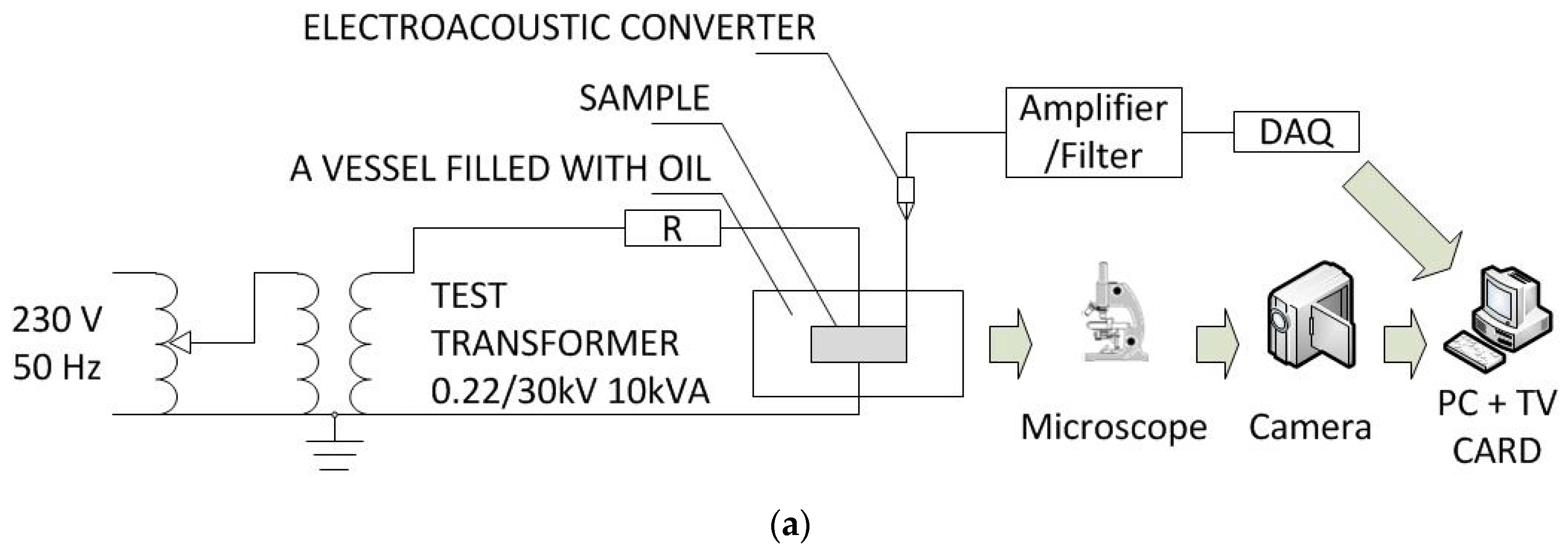
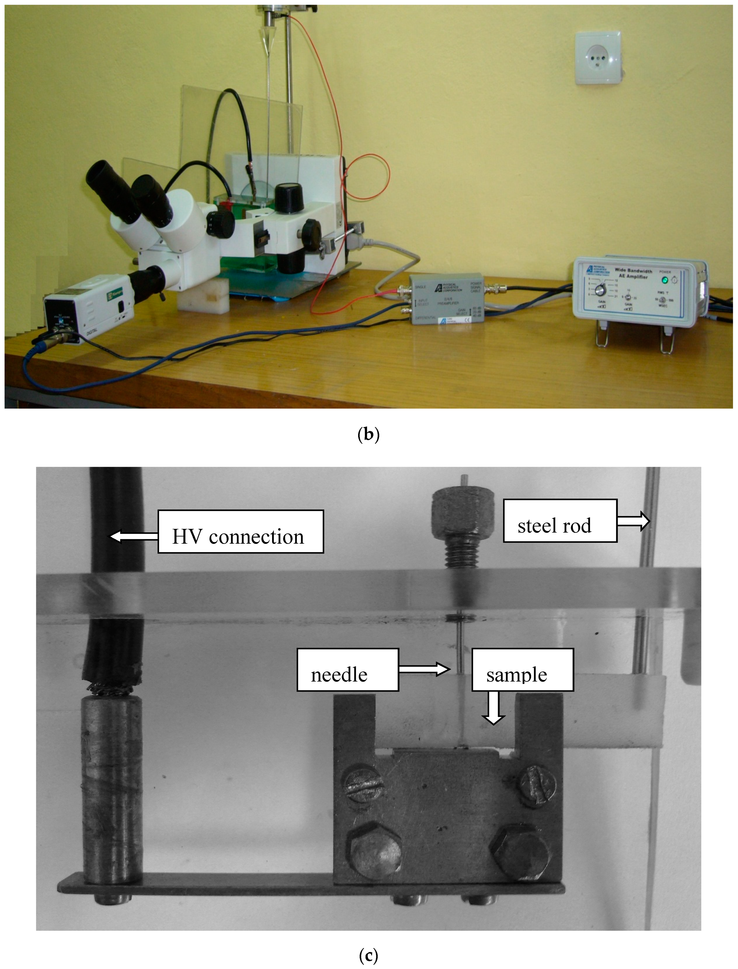
2. Test Setup and the Course of the Experiment

The first stage of the studies involved measurements of acoustic emission signals in electrically-stressed epoxy resin samples. The samples had cubicoid shapes of 25 mm × 10 mm × 4 mm. One sample surface of 25 mm × 4 mm was ground and coated with varnish conducive to electric current.

Since the process of tree channels forming in a dielectric may last very long, an electrode made of a T10 surgical needle with liquid resin poured inside the sample during sample formation was used, such that the distance between the sample bottom and the electrode end ranged from 1–3 millimeters. The procedure allowed obtaining the electric field intensity between the needle electrode and the electrode applied to the bottom of the sample, which was high enough to reduce the tree-forming duration to a few hours. The needle was connected to the neutral terminal of the transformer. The opposite base of the sample was adjacent to a plane copper electrode. The electrode was connected through a resistor of 0.5 MΩ resistance to a high-voltage terminal of a test transformer with the ratio of 220 V/30 kV and power of 10 kVA. The voltage was measured with an electrostatic voltmeter.

As part of the tests, acoustic signals were recorded for a dozen or so samples in which, under the influence of a high intensity of the electric field, the process of forming an electric tree began. The measurements were made for variable values of the supply voltage with a 50-Hz frequency and different distances between the electrodes.

The elastic waves of acoustic frequencies were emitted from the analyzed sample through a wave-guide made of a steel rod of 2 mm in diameter. One of its ends was put into a hole bored in the sample, while the other was connected to an electroacoustic converter.

As regards measurement time, the studied sample was placed in a methyl polymethacrylate vessel filled with electrical insulating oil. The voltage between the electrodes during the tests ranged from a few to several kV. The AE signals were measured by means of a Physical Acoustic Corporation (PAC) R3α electroacoustic converter and a filtering and amplifying system composed of 2/4/6 type pre-amplifier from PAC, a 20 ÷ 1000 kHz transmission band filter, and PAC AE5A amplifier. Upon amplification, the signal was recorded in the computer memory with an data acquisition (DAQ) NI–USB6251 card, which enabled signal recording with a sampling frequency up to 1 MS/s and 16-bit resolution. The test setup schema, the view of the measuring equipment, and the view a sample holder are presented respectively in Figure 1a–c.

To ensure that the recorded signals concerned the electrical treeing while we were preparing the experiment, we also tested and observed under a microscope different states of the system, i.e., without any PDs, with corona, etc. We noticed that each of the PD types was connected with different waveforms of signals, and this can be found also in different researchers’ results [35]. After that test, we rebuilt/reconfigured the setup and chose a voltage range to be sure that other types of PDs would not be present. Physically, electrical treeing is a combination of chemical and physical changes inside the specimen, so no one can be sure whether that particular signal is connected with the breaking polymer chain or PD inside the existing channel.

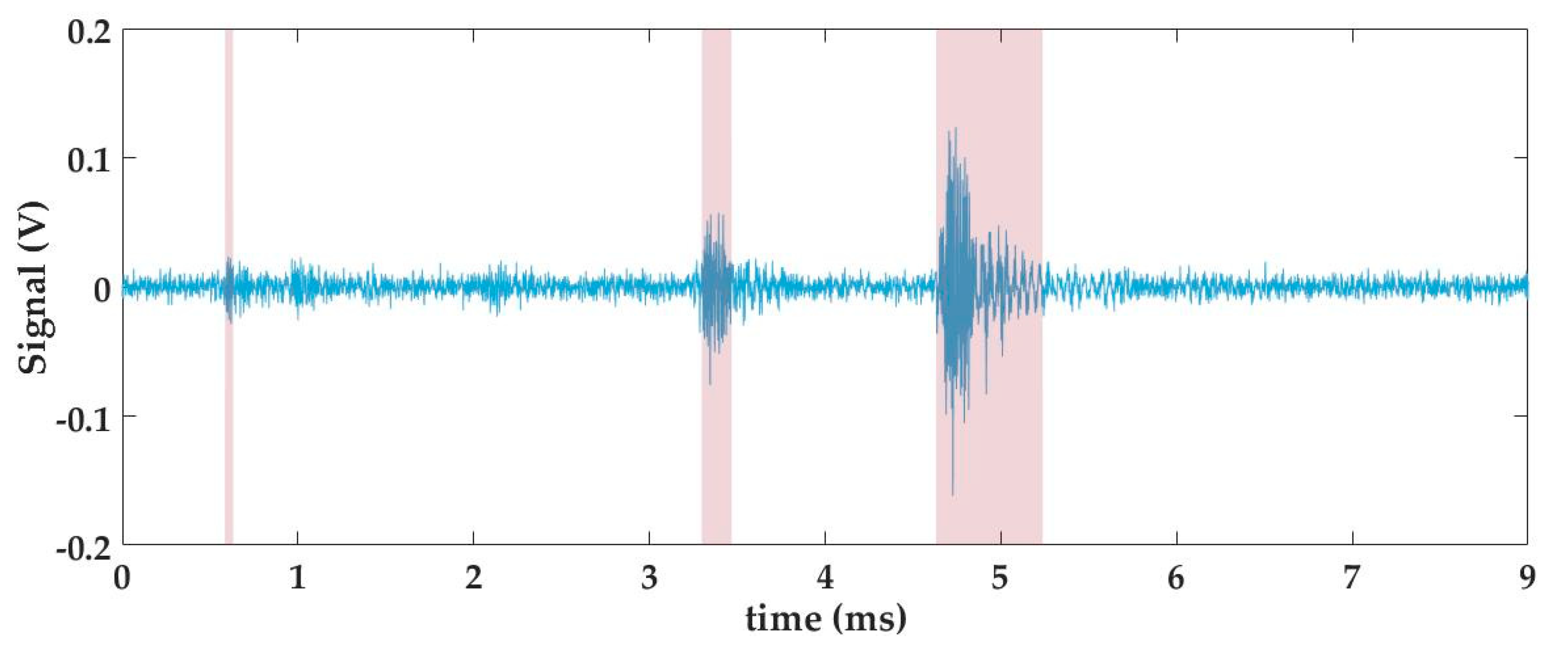
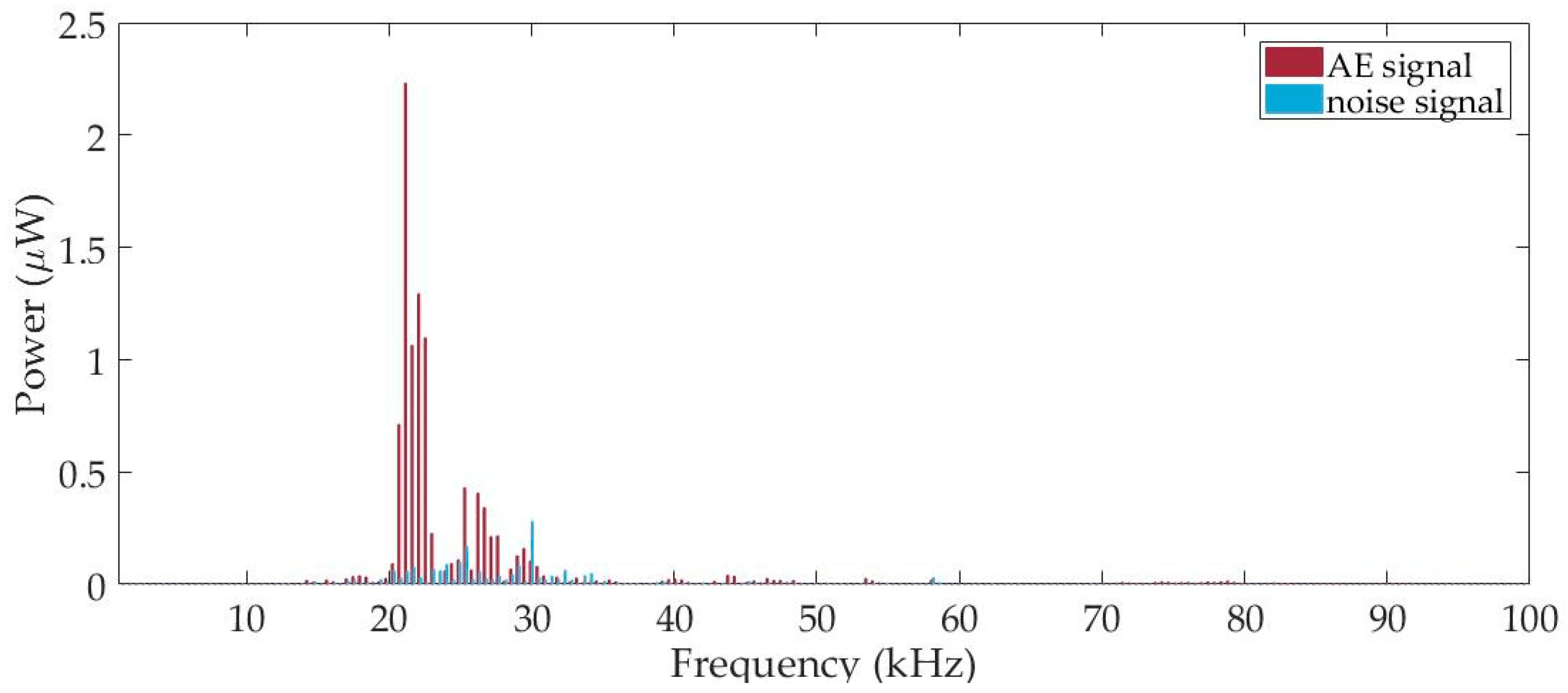
3. Method of Features’ Extraction

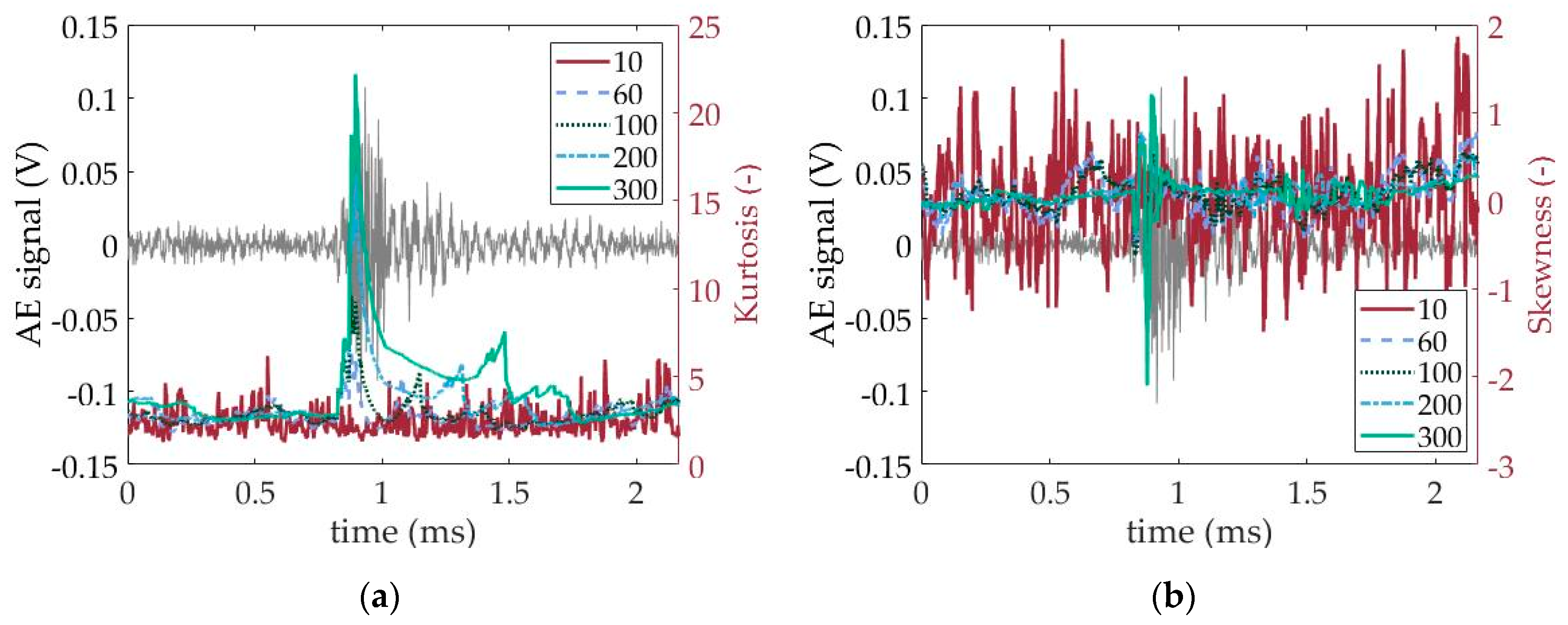
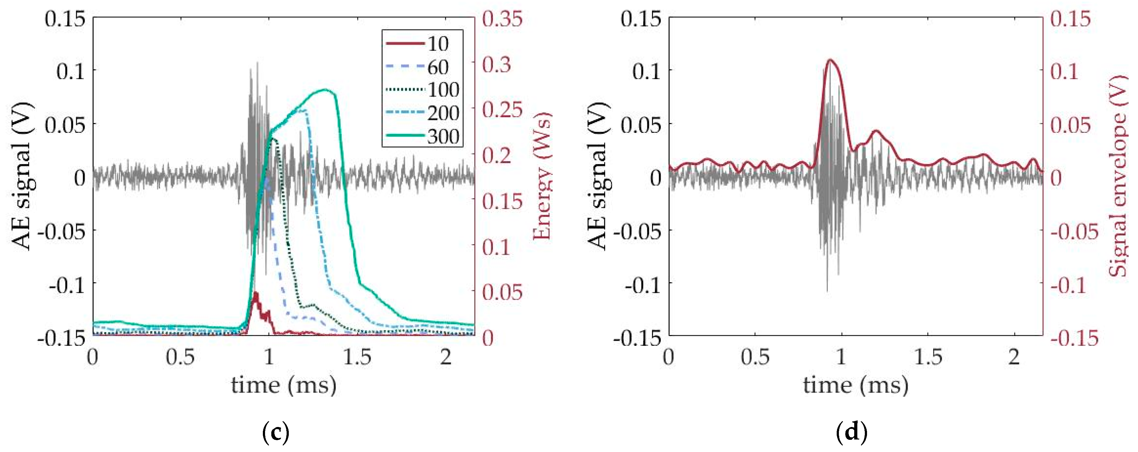
3.1. Features’ Definition

In order to extract the teaching data for neural classifiers, the analyzed signal fragment was divided into x blocks with N length of samples, where:

$$\mathit{x}=\left\{x_1,\dots ,x_n,\dots ,x_N\right\}.$$

(1)

For each x signal block, a set of statistical parameters typically used in the analysis of AE signals was identified [36,37], which was further used as input data for the neural network. The following parameters were used: signal energy (e), band power (p_BP), signal upper envelope (env), skewness (skew), and kurtosis (kurt).

The signal energy is identified based on the following relationship:

$$e={\displaystyle {\sum }_{n=1}^N{x}_n^2}$$

(2)

Skewness, as the probability distribution asymmetry measure, is identified in the following way:

$$skew=\frac{\overline{x}-med\left(\mathit{x}\right)}{\sqrt{\sigma }}$$

(3)

where $\overline{x}$ is the mean value of samples, med (x) the block median, and $\sigma$ the sample block variance.

Kurtosis, which is the measure of the results’ concentration around the mean, amounts to:

$$kurt=\frac{{\mu }_4}{{\sigma }^4}-3$$

(4)

where µ₄ is the fourth central moment of samples in the block and $\sigma$ the sample block variance. A teaching data vector d was identified for each x signal sample block, where:

$$\mathit{d}=\left\{e,p_{BP}^{},env,skew,kurt\right\}$$

(5)

In order to obtain training information y, which belongs to the set {0,1}, the recorded signal was blasted using the wavelet decomposition with the fifth-order Daubechies wave. Then, using the method of exceeding the trigger threshold, which was set at 20 mV for the presented problem, the information value y was allocated for each training set: 0 for no acoustic emission and 1 for the acoustic emission event (these are the red areas in Figure 2). Figure 2 presents one signal fragment with the sampling frequency of 1 MS/s selected for further studies. The red areas mark acoustic emission events determined on the basis of threshold crossing.

3.2. Passband Power

The selection of the band used for identifying band power p_BP was made based on the averaged spectrum for the recorded AE signals. Figure 3 presents an averaged spectrum for 1000 AE signals recorded and the spectrum of a selected signal fragment where no acoustic emission was observed. For both spectrums, the transfer function of the selected detector (R3α), given in the calibration datasheet, was taken into account.

The presented spectrum was used to select a signal band with a frequency ranging from 15 kHz–30 kHz for further analysis because the power of the signal recorded within the band increased significantly when acoustic emission occurred.

3.3. Block Length

Selecting the right length of signal blocks to study is among the most important factors affecting classification quality. When performing an analysis using a taught network, we are not able to predict if the analyzed signal block starts before, during, or at the end of the acoustic emission signal, because it is necessary to know the influence of the signal window position against the acoustic signal on the values of selected network teaching features.

In order to identify the aforementioned relationships, window lengths of 10, 60, 200, and 300 samples were used. The windows were applied to a signal containing a single acoustic emission and moved by one sample (the window position against the AE signal was changed this way). A dataset was calculated for each position of the window. Figure 4 presents the values of each teaching feature as a function of the window position, at different window lengths, against the AE signal: kurtosis (a), skewness (b), and energy (c) respectively. Moreover, Figure 4c presents the identified upper envelope of the sample signal.

3.4. Principal Component Analysis

Principal component analysis (PCA) is a statistical method for factor-based analysis. A collection N of K variable observations is analyzed as a collection of N points distributed in a K-dimensional space. Using the distribution of singular values for the deviation covariance matrix, it is possible to develop a new system that maximizes the variance of subsequent coordinates. This way, it is possible to reduce the space size (decrease the number of the analyzed input data) [30] and the size of the neural network, while maintaining the highest possible amount of information regarding the input process.

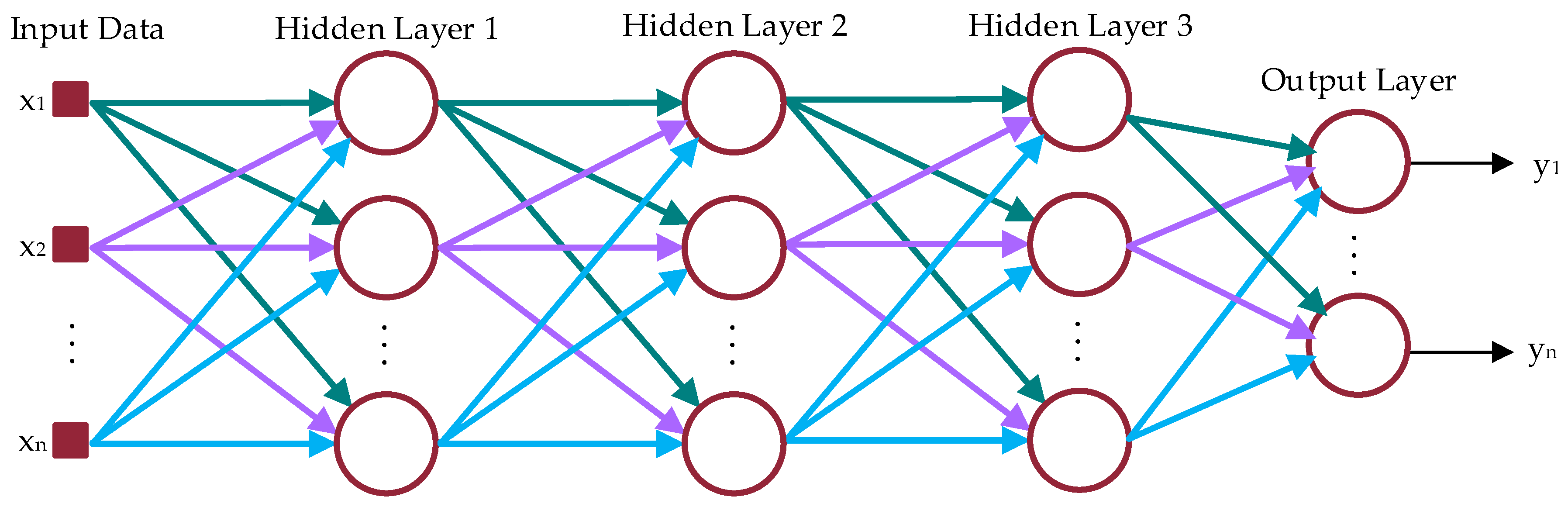
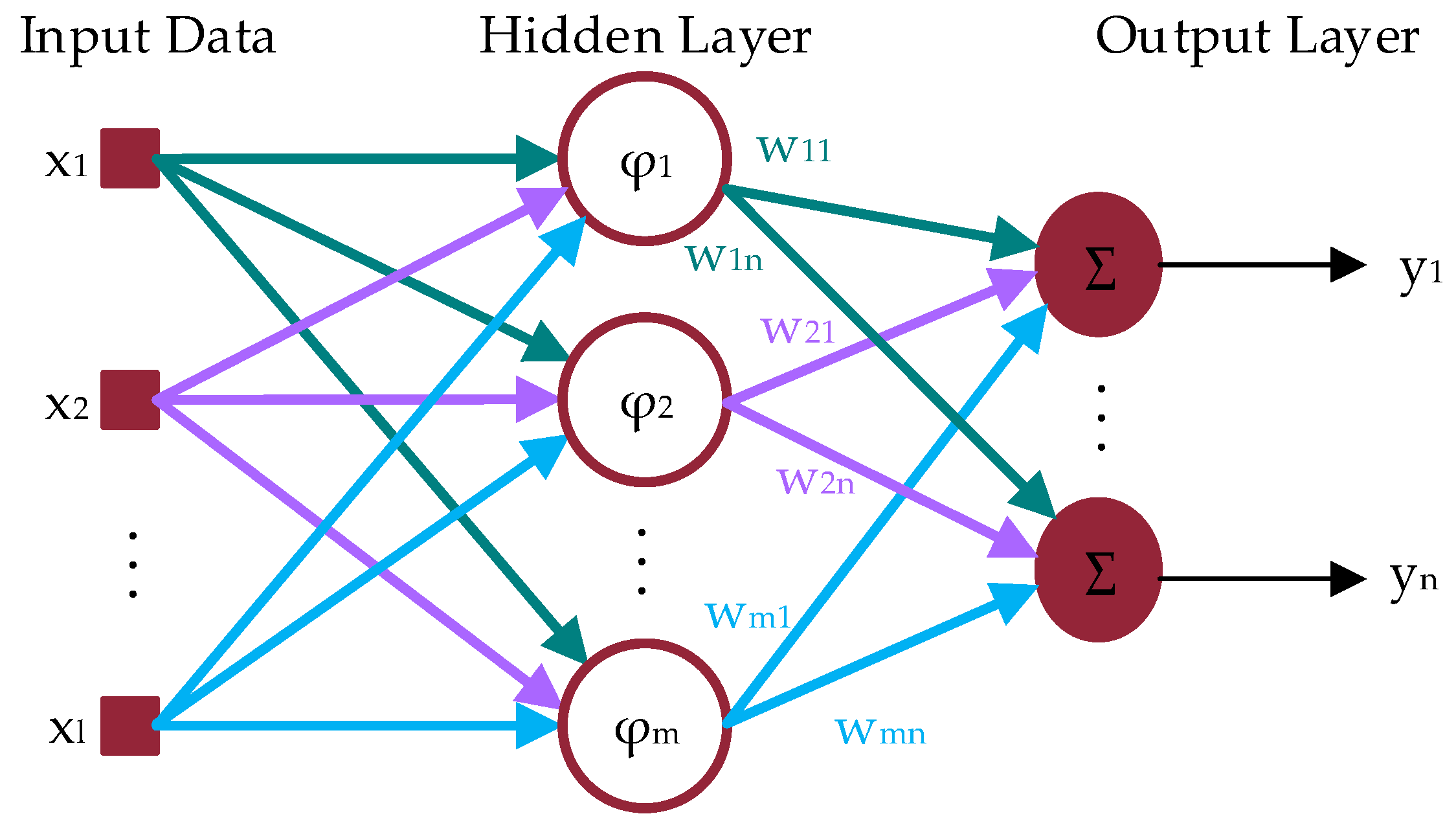
4. Artificial Neural Network Classifiers Used to Select EA Signals

4.1. Feedforward Neural Network

In a forward non-linear neural network (FNN), the flow of information (signals) is unidirectional. Its structure consists of the input layer, two or more hidden layers, and the output layer (Figure 5). All layer inputs can be linked only with the neurons in the preceding layer. Input signals x in a neuron are added to weights w. Neuron y’s output signal is calculated using a non-linear activation function φ, according to the relationship [38]:

$$y=\phi \left({\displaystyle \sum _{m=1}^M{w}_m{x}_m}\right)$$

(6)

The unipolar sigmoid function is among the most commonly-used activation functions:

$$\phi \left(z\right)=\frac{1}{1+e^{-z}}$$

(7)

alongside a bipolar function (hyperbolic tangent):

$$\phi \left(z\right)=\frac{1-e^{-z}}{1+e^{-z}}$$

(8)

For learning feedforward neural network (FFN), the Levenberg–Marquardt algorithm was used. This method is one of the most effective learning algorithms. It has high convergence when network weights are near the optimal solution (as the Gauss–Newton method) and when the network is far from the optimal solution (as the descent gradient method). Detailed information about the Levenberg–Marquardt algorithm can be found in [39].

4.2. Radial Basis Functions

A radial basis functions (RBF) network, similar to FNN, is a network with an oriented flow of signals. The network neurons have a radial activation function φ. The neuron output y is described by the relationship [40]:

$$y_j\left(\mathit{x}\right)={\displaystyle \sum _i^m{w}_{ij}\phi \left(\Vert \mathit{x}-{\mathit{c}}_i\Vert \right)}$$

(9)

where i is the hidden layer neuron number, j the radial network output number, w_ij the coefficient of the weight, x the input data vector, and c_i the center of the radial function for the ith neuron of the hidden layer.

In such a neuron, the value of the output signal is not proportional to the scalar product of x inputs and w neuron weights, but inversely proportional to the distance between x and the central point of radial function c located at the hyperspace of the network input parameters. The Gaussian function is among the most commonly-used radial functions. Figure 6 presents the structure of an RBF network.

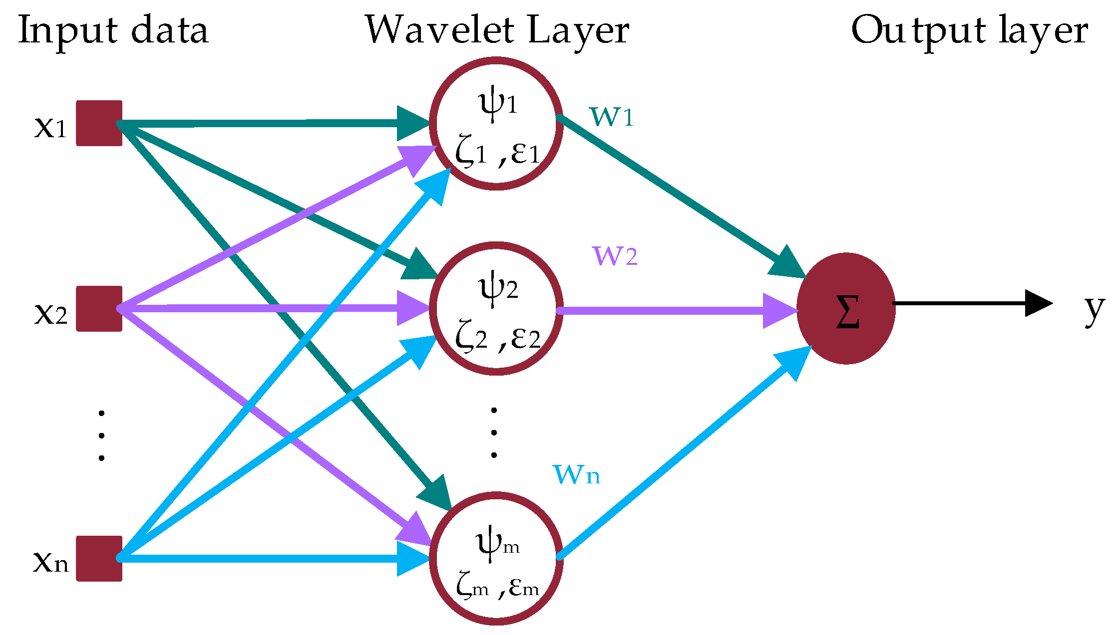
4.3. Wavelet Neural Network

A wavelet neural network (WNN) structure consists of an input, output, and hidden layer of wavelet neurons (Figure 7).

The function of wavelet neurons’ activation φ is described by the relationship [41]:

$$\phi \left(\mathit{x}\right)={\displaystyle \prod _i^m\psi \left(\frac{x_i-{\zeta }_i}{{\epsilon }_i}\right)}.$$

(10)

where x is the input signal vector, ψ the wavelet function, ζ the translation parameter, and ε the scale parameter.

The process of such network teaching involves the selection of the scale parameters and shifting each wavelet ψ used inside a wavelet neuron nucleus. For the study, the authors used Mexican hat wavelet function.

Contrary to other network types, drawing of the initial values of the wavelet parameters ζ and ξ may result in the teaching algorithm being stuck in the local minimum. That is why network teaching is preceded by the initialization of initial parameters. A feature selection method developed by Oussar and Dreyfus was used for the study [42]. It consists of the following steps:

• Step 1: creating a library of wavelets with different parameters.
• Step 2: removing those wavelets not falling within the variability range of each input parameter.
• Step 3: developing a ranking of wavelets and iterative selection of the best wavelets using the Gram–Schmidt ortho-normalization algorithms.

Subsequently, fully-initialized WNN was learned with the backpropagation algorithm. A detailed description of the WNN’s structure and learning algorithm used for the study can be found in [41].

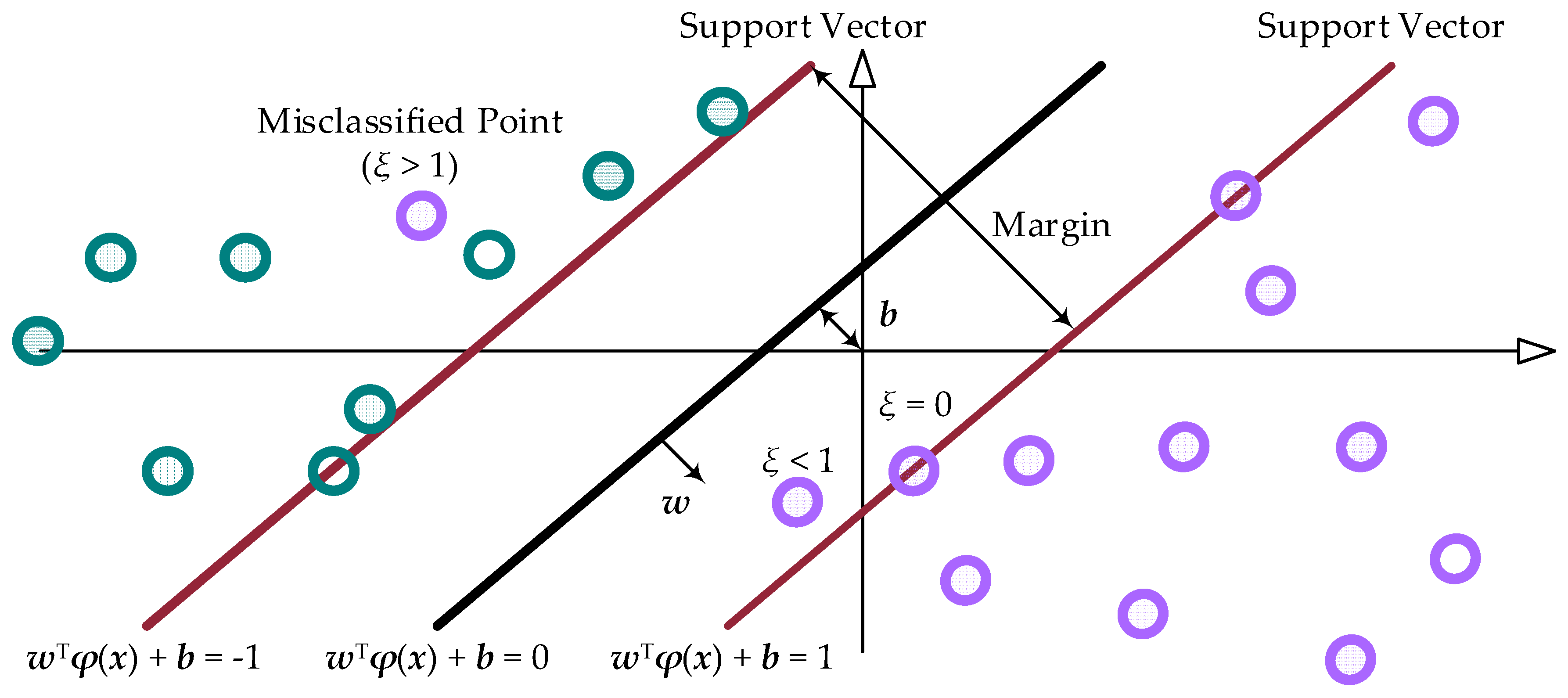
4.4. Support Vector Machine

A support vector machine (SVM) was another network used in the studies. The purpose of the SVM network operation is to use a hyperplane spread in the hyperspace of the input parameters, which separates a collection of points (sets of input parameters) belonging to two different classes, with a certain error margin.

It is a type of binary classifier. Its operating principle can be presented on the example of a network with two input parameters x = (x₁, x₂). Figure 8 presents the operating principle of such a classifier. The points lying in the plane (x₁, x₂) are divided into two classes marked in green and viloet. The SVM classifier searches for a straight line (black line in the drawing), which will maximize the error margin limited on both sides of the curve with support vectors, the brown lines in the drawing. The points exceeding the limits of the error margin will be misclassified. The purpose of SVM teaching is to select the coefficients of the straight line separating the points in such a way that the error margin is maximized (distance between the support vectors). Algorithms of non-linear optimization with constraints, and Lagrange’s method in particular, were used for the network teaching [43].

5. Results

Each of the described networks was taught in order to classify the signals into two groups: that which contains and that which does not contain acoustic emission signals accompanying dielectric treeing. The previously-described properties were used to develop teaching data for the blocks with the following lengths: 10, 60, 100, 200, and 300 samples.

In the first part of the results, classification efficiency was specified for a test fragment of the signal other than the network teaching signal. In the second section, the signal classification efficiency was presented for the teaching data reduced by means of PCA.

Additionally, the optimum size of the network was achieved in the cross-validation, which consisted of dividing the set of reference data into equinumerous k subsets. The network with a given number of neurons was learned on the basis of k-1 subsets, and the unused subset was the validation data. This process was repeated k times. Thus, the obtained k learning outcomes networks were averaged.

5.1. Classifier Efficiency Analysis

Each network taught was subjected to a test developed based on a random signal fragment.

Table 1. Classification efficiency test results for variable data block lengths. WNN, wavelet neural network.

Network Type	Block Length (Samples)	Neurons	Efficiency (%)	Network Type	Block Length (Samples)	Efficiency (%)
FFN	10	10	97.2	SVM	10	90.4
	60	14	97.6		60	87.8
	100	16	97.3		100	88.5
	200	15	97.5		200	95.6
	300	11	96.7		300	96.3
WNN	10	3	90.9	RBF	10	95.8
	60	3	88.2		60	95.3
	100	3	86.2		100	94.6
	200	2	94.7		200	94.8
	300	3	95.7		300	95.6

presents the classification efficiency for each network type at variable block lengths based on which, calculations were made.

5.2. Classification Using PCA

Since the most stable efficiency results for each network were obtained for the data identified based on the block length of 300 samples, the data were subjected to PCA, and PCs were developed from them.

Table 2. Classification efficiency test results for variable data block lengths.

PC	Variance (–)	Variance Share (%)
1st	3.6092	98.17
2nd	0.0606	1.65
3rd	0.0066	0.18
4th	6.3 × 10−5	0
5th	8.7 × 10−11	0

shows variances for different components and their percent share in the total variance.

Based on the results presented in the table above, it can be concluded that the share of the first primary component in the whole signal amounted to over 98%, which denotes the possibility to reduce a system of five decisive variables to only one variable with no significant information loss.

Table 3. Classification efficiency test results for variable data block lengths.

PC Number	Efficiency (%)
	FFN	WNN	RBF	SVM
1	96.6	95.5	95.7	96.2

presents the efficiency of the analyzed networks for teaching when only the first primary component was used.

6. Discussion

The paper proposed the use of ANN for the analysis of acoustic signals accompanying electrical treeing in epoxy resin.

The recorded signals were divided into blocks used to identify the values of the teaching data. Then, the features of the reference signal were analyzed using a moving window of a set length.

The features were divided into two groups whose properties depended on window length and position versus the beginning of the AE pulse. Hence, kurtosis and skewness, due to the high dynamics of changes, can be good indicators for the identification of the beginnings of AE pulses related to treeing. The values of the parameters, however, did not reflect the duration of AE signals, and their use required the application of an analysis window with a minimum length. In the analyzed case, the results were regarded as satisfactory and repeatable for window lengths over 200 samples.

The other group of analyzed parameters, which describes the signal by its power characteristics, i.e., band power and signal energy, demonstrated elevated values during the signal. The steepness of the signal energy increase did not depend on the analysis of the window length, but a relevant selection of the length helped to identify the place in the signal where the signal amplitude dropped significantly. This is seen in the diagram as an inflexion point.

Since AEs in electrical treeing are related to the breaking of polymer chains or the presence of partial discharge in the existing channels, the value and dynamics of signal energy changes during a single pulse can be linked to treeing intensity.

By analyzing the results for each neural network, one can see that FFN demonstrated the highest efficiency. Slightly poorer results were obtained for RBF, WNN, and SVM. Moreover, for FFN and RBF, the results for each window length applied to the signal were comparable. WNN and SVN rendered better results for the greater analysis of window lengths. Moreover, WNN in its realization used only two wavelet neurons, while the structure of FNN required at least 15 neurons.

In the case of networks taught by means of the first primary component, one can state that the efficiency of each network dropped by a value that did not exceed 0.5%.

Summing up, the high efficiency in detecting AE signals accompanying electrical treeing needs to be highlighted. In order, however, to obtain as much information as possible on the AE pulse course, it seems justified to use an algorithm based on the following three stages:

-

signal envelope analysis,

-

AE signals’ detection,

-

analysis of individual signals.

A signal envelope analysis could provide hints for identifying the optimum window length at the discrimination level assumed on an arbitrary basis.

The performed experiments revealed that ANN can be successfully used for signal detection and classification, with the kurtosis, skewness, and energy of a single signal as the classifying parameters.

The effectiveness of the applied method was confirmed by the results obtained for various electrical parameters, i.e., different inter-electrode distances and different intensity of the electric field in this space. Regardless of the values of the above parameters, the results of AE signal identification were characterized by equally high efficiency, which proves the correctness of the assumptions made. The next stage covered a detailed analysis of the signals classified in the previous step with regard to the criteria assumed by the experimenter.

The completed analyses justify the usefulness of further studies on using ANN for partial discharge analysis and electrical treeing for solid dielectrics.

This knowledge could be of particular value to persons making diagnoses on the condition that the proposed method could be used online. That is why future efforts should focus on developing algorithms that would satisfy this demand.

References

1. Rayner, E.H. High-voltage tests and energy losses in insulating materials. Br. JIEE 1912, 49, 3. [Google Scholar] [CrossRef]
2. Robinson, D.M. Dielectric Phenomena in High Voltage Cables; Chapman Hall Ltd.: London, UK, 1936. [Google Scholar]
3. Whitehead, S. Breakdown of Solid Dielectrics; Ernest Benn: London, UK, 1932. [Google Scholar]
4. Bahder, G.; Daking, T.W.; Lawson, J.H. Analysis of treeing type breakdown. In Proceedings of the International Conference on Large High Voltage Systems, Paris, France, 25 August–2 September 1976; pp. 709–714. [Google Scholar]
5. Grzybowski, S.; Dobroszewski, R. Influence of partial discharges of the development of electrical treeing in polyethylene insulated cables. In Proceedings of the International Symposium on Electrical Insulation, Philadelphia, PA, USA, 21–26 July 1978; pp. 122–125. [Google Scholar]
6. Noskov, M.D.; Malinovski, A.S.; Sack, M.; Schwab, A.J. Modelling of partial discharge development in electrical tree channels. IEEE Trans. Dielectr. Electr. Insul. 2003, 10, 425–434. [Google Scholar] [CrossRef]
7. Jocteur, T.; Osty, M.; Lemanique, H.; Terramorsi, G. Research and Development in France in the Field of Extruded Polyethylene Insulated High Voltage Cables. In Proceedings of the International Conference on Large High Tension Electric Systems, Reference 21-07. Paris, France, 28 August–6 Septembet 1972; pp. 1–22. [Google Scholar]
8. Kreuger, F.H.; Bentvelsen, P.A.C. Breakdown Phenomena in Polyethylene Insulated Cables. In Proceedings of the International Conference on Large High Tension Electric Systems, Reference 21-05. Paris, France, 28 August–6 Septembet 1972; pp. 1–7. [Google Scholar]
9. Tykociner, J.T.; Brown, H.A.; Paine, E.B. Oscillations due to ionization in dielectrics and methods of their detection and measurement. Univ. Illinois Bull. 1933, 30. [Google Scholar]
10. Tian, Y.; Lewin, P.L.; Davies, A.E.; Sutton, S.J.; Swingler, S.G. Application of acoustic emission techniques and artificial neural networks to partial discharge classification. In Proceedings of the Conference Record of the 2002 IEEE International Symposium on Electrical Insulation, Boston, MA, USA, 7–10 April 2002; pp. 119–123. [Google Scholar]
11. Dissado, L.A. Understanding electrical trees in solids: From experiment to theory. IEEE Trans. Dielectr. Electr. Insul. 2002, 9, 483–497. [Google Scholar] [CrossRef]
12. Eichhorn, R.M. Treeing in solid extruded electrical insulation. IEEE Trans. Electr. Insul. 1977, 12, 2–18. [Google Scholar] [CrossRef]
13. Shimizu, N.; Laurent, C. Electrical tree initiation. IEEE Trans. Dielectr. Electr. Insul. 1998, 5, 651–659. [Google Scholar] [CrossRef]
14. Shimizu, N.; Uchida, K.; Rasikawan, S. Electrical tree and deteriorated region in polyethylene. IEEE Trans. Electr. Insul. 1992, 27, 513–518. [Google Scholar] [CrossRef]
15. Kudo, K. Fractal analysis of electrical trees. IEEE Trans. Dielectr. Electr. Insul. 1998, 5, 713–727. [Google Scholar] [CrossRef]
16. Dissado, L.A.; Dodd, S.J.; Champion, J.V.; Williams, P.I.; Alison, J.M. Propagation of electrical tree structures in solid polymeric insulation. IEEE Trans. Dielectr. Electr. Insul. 1997, 4, 259–279. [Google Scholar] [CrossRef]
17. Opydo, W.; Dobrzycki, A. Detection of electric treeing of solid dielectrics with the method of acoustic emission. Electr. Eng. 2012, 94, 37–48. [Google Scholar] [CrossRef]
18. Dobrzycki, A.; Opydo, W. An attempt to appraise the progress of methyl polymethacrylate degradation induced by a strong electric field on the grounds of analysis of acoustic signal emission. Pozn. Univ. Technol. Acad. J. 2007, 57, 197–203. [Google Scholar]
19. Markalous, S.M.; Tenbohlen, S.; Feser, K. Detection and Location of Partial Discharges in Power Transformers using Acoustic and Electromagnetic Signals. IEEE Trans. Dielectr. Electr. Insul. 2008, 15, 1576–1583. [Google Scholar] [CrossRef]
20. Lundgaard, L.E. Partial discharge. XIV. Acoustic partial discharge detection-practical application. IEEE Electr. Insul. Mag. 1992, 8, 34–43. [Google Scholar] [CrossRef]
21. Casals-Torrens, P.; Gonzalez-Parada, A.; Bosch-Tous, R. Online PD detection on high voltage underground power cables by acoustic emission. Procedia Eng. 2012, 35, 22–30. [Google Scholar] [CrossRef] [Green Version]
22. Dobrzycki, A.; Opydo, W.; Zakrzewski, S. Acoustic emission signals associated with prebreakdown state in air high voltage insulating systems. Comput. Appl. Electr. Eng. 2015, 13, 278–286. [Google Scholar]
23. Boczar, T.; Borucki, S.; Cichon, A.; Zmarzly, D. Application Possibilities of Artificial Neural Networks for Recognizing Partial Discharges Measured by the Acoustic Emission Method. IEEE Trans. Dielectr. Electr. Insul. 2009, 16, 214–223. [Google Scholar] [CrossRef]
24. Candela, R.; Mirelli, G.; Schifani, R. PD recognition by means of statistical and fractal parameters and a neural network. IEEE Trans. Dielectr. Electr. Insul. 2000, 7, 87–94. [Google Scholar] [CrossRef]
25. Dobrzycki, A.; Mikulski, S.; Opydo, W. Analysis of acoustic emission signals accompanying the process of electrical treeing of epoxy resins. In Proceedings of the ICHVE 2014—2014 International Conference on High Voltage Engineering and Application, Poznan, Poland, 8–11 September 2014. [Google Scholar]
26. Dobrzycki, A.; Mikulski, S. Using of wavelet transform in the analysis of AE signals accompanying the process of epoxy resins electrical treeing. Przegląd Elektrotechniczny 2016, 1, 223–225. [Google Scholar] [CrossRef]
27. Mohanty, S.; Ghosh, S. Artificial neural networks modelling of breakdown voltage of solid insulating materials in the presence of void. IET Sci. Meas. Technol. 2010, 4, 278–288. [Google Scholar] [CrossRef]
28. Mathur, L.S.; Agrawal, A.; Singh, D.K. Modeling of Breakdown Voltage of Solid Insulating Materials by Artificial Neural Network. Int. J. Eng. Sci. Res. Technol. 2016, 5, 788–796. [Google Scholar]
29. Masood, A.; Zuberi, M.U. Correlation of Breakdown Strength Parameters of Solid Insulation using Artificial Neural Network (ANN). Eur. J. Adv. Eng. Technol. 2016, 3, 14–19. [Google Scholar]
30. Tsangouri, E.; Aggelis, D.G.; Matikas, T.E.; Mpalaskas, A.C. Acoustic Emission Activity for Characterizing Fracture of Marble under Bending. Appl. Sci. 2016, 6, 6. [Google Scholar] [CrossRef]
31. Świt, G. Acoustic Emission Method for Locating and Identifying Active Destructive Processes in Operating Facilities. Appl. Sci. 2018, 8, 1295. [Google Scholar] [CrossRef]
32. Ebrahimkhanlou, A.; Salamone, S. Single-sensor acoustic emission source localization in plate-like structures: A deep learning approach. In Proceedings of the Health Monitoring of Structural and Biological Systems XII, Denver, CO, USA, 5–8 March 2018; Kundu, T., Ed.; SPIE: Bellingham, WA, USA, 2018; p. 59. [Google Scholar]
33. Ebrahimkhanlou, A.; Salamone, S. Single-Sensor Acoustic Emission Source Localization in Plate-Like Structures Using Deep Learning. Aerospace 2018, 5, 50. [Google Scholar] [CrossRef]
34. Ebrahimkhanlou, A.; Choi, J.; Hrynyk, T.D.; Salamone, S.; Bayrak, O. Detection of the onset of delamination in a post-tensioned curved concrete structure using hidden Markov modeling of acoustic emissions. In Proceedings of the Sensors and Smart Structures Technologies for Civil, Mechanical, and Aerospace Systems 2018, Denver, CO, USA, 5–8 March 2018; Sohn, H., Ed.; SPIE: Bellingham, WA, USA, 2018; p. 74. [Google Scholar]
35. Sikorski, W. The detection and identification of partial discharges in power transformer with the use of the acoustic emission method. Przegląd Elektrotechniczny 2010, 86, 229–232. [Google Scholar]
36. Lin, L.; Xu, Q.; Zhou, Y. Extracting the Fault Features of an Acoustic Emission Signal Based on Kurtosis and Envelope Demodulation of Wavelet Packets. In Advances in Acoustic Emission Technology; Springer: Cham, Switzerland; pp. 101–111.
37. Mohammad, M.; Abdullah, S.; Jamaludin, N.; Nuawi, M.Z. Correlating Strain and Acoustic Emission Signals of Metallic Component Using Global Signal Statistical Approach. In Proceedings of the Materials and Manufacturing Technologies XIV, Istanbul, Turkey, 13–16 July 2011; Yigit, F., Hashmi, M.S.J., Eds.; Volume 445, p. 1064+. [Google Scholar]
38. Schmidhuber, J. Deep learning in neural networks: An overview. Neural Netw. 2015, 61, 85–117. [Google Scholar] [CrossRef] [Green Version]
39. Bishop, C.M. Pattern Recognition and Machine Learning; Springer: Berlin, Germay, 2006; ISBN 9780387310732. [Google Scholar]
40. Buhmann, M.D. Radial Basis Functions; Cambridge University Press: Cambridge, UK, 2003; ISBN 9780511543241. [Google Scholar]
41. Alexandridis, A.K.; Zapranis, A.D. Wavelet neural networks: A practical guide. Neural Netw. 2013, 42, 1–27. [Google Scholar] [CrossRef] [Green Version]
42. Oussar, Y.; Dreyfus, G. Initialization by selection for wavelet network training. Neurocomputing 2000, 34, 131–143. [Google Scholar] [CrossRef] [Green Version]
43. Cristianini, N.; Scholkopf, B. Support vector machines and kernel methods—The new generation of learning machines. AI Mag. 2002, 23, 31–41. [Google Scholar]
Figure 1. The test setup schema (a), view of the measuring equipment (b), and view of the sample holder (c) for measuring acoustic signals accompanying the treeing of solid dielectrics.
Applsci 09 01523 g001aApplsci 09 01523 g001b
Figure 2. Fragment of the recorded signal where dielectric degradation occurred.
Applsci 09 01523 g002
Figure 3. Averaged signal spectrum for 1000 recorded acoustic emission signals and measurement noise spectrum.
Applsci 09 01523 g003
Figure 4. Influence of the position of different window lengths against the AE signal on the teaching properties’ values: kurtosis (a); skewness (b); energy (c); upper envelope (d); the recorded signal wavelength is in the background.
Applsci 09 01523 g004aApplsci 09 01523 g004b
Figure 5. Sample structure of a feedforward network with three hidden layers.
Applsci 09 01523 g005
Figure 6. RBF network diagram.
Applsci 09 01523 g006
Figure 7. Wavelet neural network structure.
Applsci 09 01523 g007
Figure 8. Principle of support vector machine operation.
Applsci 09 01523 g008