Abstract
Assessing the seismic vulnerability of large numbers of buildings is an expensive and time-consuming task, requiring the collection of highly complex and multifaceted data on building characteristics and the use of sophisticated computational models. This study reports on the development of a data mining technique: Support Vector Machine (SVM) for resolving such multi-dimensional data problems for assessing buildings’ seismic vulnerability at a regional scale. Particularly, we developed an SVM model for rapid assessment of the macroscale seismic vulnerability of buildings in terms of spectral yield and ultimate points of their capacity curves. Two case studies, one with 11 building characteristics and the other with 20, were used to test the proposed SVM model. The results show that when 20 building characteristics are included, an individual building’s seismic vulnerability in term of its spectral yield and ultimate points can be predicted by the proposed SVM model with an average 64% accuracy if the training dataset contains 400 samples, rising to 74% with 4400 training samples. Coupling the proposed technique with demand curves based on buildings’ locations will enable rapid and reliable seismic-risk assessment at a regional scale, requiring only basic building characteristics rather than complex computational models.
1. Introduction
Earthquake risk to people and property is primarily conceptualized as a function of buildings’ seismic vulnerability [1]. Assessment of the seismic vulnerability of buildings at a city, regional, or national scale has traditionally been expensive and time-consuming, requiring highly complex and multifaceted data on building characteristics as well as sophisticated computational models. For the assessment of buildings’ seismic risk at a regional scale, catastrophe risk modeling (CRM) has been widely used. CRM typically consists of four modules—hazard, exposure, vulnerability, and loss—with risk estimated as the impacts of a hazard that exploits the vulnerabilities of a system of interest on its exposure to that hazard [2]. In the case of earthquakes, the hazard module determines the characteristics of the potential seismic events that would affect the system and the exposure module collects data on the geological and built environment. Then, based on the information collected in the exposure module, the seismic vulnerabilities of buildings are determined in the vulnerability module. Finally, through the various loss-interpretation models included in the fourth module, building damage can be translated into specific types of losses.
Gradual improvements have been made in hazard modules’ ability to estimate the locations and return periods of seismic events, and exposure module by using advanced geographic information system for data collection [3,4,5]. However, the vulnerability module has proved an impediment to the effective use of CRM for seismic-risk assessment. Computational models for simulating a building’s seismic vulnerability, such as static push-over or non-linear dynamic models, are costly in both time and economic terms, requiring highly complex and multifaceted data on each building’s structural configuration and material properties. Moreover, for these types of computational analysis to be applied at a regional scale, they must be repeated thousands of times. Thus, based on a data-mining (DM) technique (SVM algorithm) that focuses on the prediction of a building’s spectral yield and ultimate acceleration-displacement points, the present study developed a methodology for rapid, macroscale assessment of buildings’ seismic vulnerability using relatively small sets of basic building characteristics. As well as addressing the inefficiency of current CRM vulnerability modules, it is hoped that the present research will serve as a basis for further macroscale studies of the vulnerability of constructed facilities facing a variety of natural hazards, and thus facilitate more accurate and rapid risk assessment.
2. Review: Regional-Scale Assessment of Buildings’ Seismic Vulnerability
This section discusses prior research on methodologies for the assessment of buildings’ seismic vulnerability at regional scales. Such approaches can be divided into the three major categories: empirical, analytical, and semi-empirical.
2.1. Empirical Vulnerability Assessment
Vulnerability curves established by post-seismic observations of buildings by type can serve as a simplified and cost-efficient means of vulnerability assessment, allowing reasonable estimations of expected damage levels at given seismic intensities [6,7,8]. However, despite their great simplicity, such empirical approaches have drawbacks in terms of both flexibility and accuracy. Firstly, since vulnerability curves are determined based on post-event surveys of damaged buildings in an affected area, they cannot be fairly applied to any building types that differ markedly from those already affected by earthquakes or that have been affected but not surveyed systematically. As such, the empirical approach is not suitable to areas of low to moderate seismic hazard or where no accurately recorded historical damage data exists. Secondly, a measurement of ground-motion intensity, such as peak ground acceleration (PGA), is commonly used as the explanatory variable in regression models that have building damage as the dependent variable, without taking into consideration the relationship between the frequency content of the ground motion and the fundamental period of vibration of buildings. Specifically, PGA is the maximum ground response of an earthquake, not the maximum response of a structure; such use of PGA can therefore lead researchers to ignore the possible effects of resonance between the frequency of an earthquake and a structure and thereby decrease the accuracy of vulnerability curves. For example, a high-rise building will have a greater response to a low-frequency earthquake than to a high-frequency one with the same PGA.
2.2. Analytical Vulnerability Assessment
Amid improvements in advanced earthquake engineering as well as computer science, computational structural modeling has served as a powerful tool for assessing buildings’ response to ground shaking. Static pushover analysis, for example, provides a practical means for evaluating inelastic structures’ displacement responses to earthquakes of given intensities [9,10,11,12]. This type of analysis generates capacity curves, which express seismic capacity in terms of the horizontal displacement of a building under increasing lateral load [13]. The seismic-demand spectrum, on the other hand, is generated based on the geotechnical and seismicity characteristics of the building’s location. A building’s performance point, found at the intersection of its capacity curve with the seismic-demand curve of its site, refers to the maximum displacement it can withstand under the given seismic-demand curve. Once its performance point is known, the failure mechanism of the building’s structure can be closely investigated, based on the ductility capacity of all structural elements under the calculated maximum displacement. Therefore, a building’s capacity curve is critically important to the representation of its seismic vulnerability.
2.3. Semi-Empirical Vulnerability Assessment
Ideally, to achieve a holistic seismic-risk assessment for an urban area, every single building’s behavior during ground shaking should be investigated via computational modeling. However, because effective computational models require complex, detailed information on the structures and materials of every building, it is not practical to apply them at the urban scale. Thus, to ensure that vulnerability assessment remains at an acceptable accuracy level, while avoiding time-consuming processes of large-scale data collection, the semi-empirical approach evaluates vulnerability based on a smaller range of selected building attributes, selected with the aid of experts and historical data. Since the aim of any large-scale vulnerability assessment is to estimate “average” performance among a group of buildings, the principle of the semi-empirical approach is to group buildings with similar seismic-vulnerability characteristics into a set of predefined building classes, each identified by a reasonable number of building characteristics.
Data collection for the selected building characteristics can be performed rapidly through visual screening [14], which has been widely in semi-empirical approaches to urban risk assessment [15,16]. Rather than seeking detailed information on structural designs or materials, visual screening involves the recording of a predefined number of visible structural parameters (usually no more than 15) observed during a sidewalk survey [17]. Vulnerability classifications or scores are then determined based on the collected building information, in combination with experts’ judgments and historical earthquake-damage data. For example, Taiwan’s National Center for Research on Earthquake Engineering (NCREE) [18] created an index of seismic resistance (ISR) from 0 to 100 based on the cumulative scores of 20 structural parameters, including soft-story effect, short-column effect, elevation and plan irregularity, state of maintenance, redundancy, and so on, and used it to investigate the vulnerabilities of 5400 school buildings. The ISR threshold was set at 80, based on empirical data including experiments and information on historical damage, and 1851 buildings that scored below 80 were classified as high vulnerability.
Semi-empirical approaches have been criticized for sacrificing too much accuracy in exchange for time savings in the data-collection phase. Nevertheless, their reasonably effective use of a limited number of essential parameters in the estimation of buildings’ vulnerability has paved the way for the application of machine-learning techniques to urban and regional-scale building-vulnerability assessment problems.
2.4. Machine Learning in Disaster-Risk Assessment
DM has been seen as a powerful alternative to conventional statistical methods when dealing with multi-dimensional big data problems, insofar as they require no assumptions to be made about data distributions [19]. An urban natural-hazard risk assessment can be conceived of as an immensely complex multi-dimensional problem whose hazard, exposure, and vulnerability modules require masses of quantitative and qualitative data. As such, SVM—a DM technique derived from statistical-learning theory—has been widely and effectively used to solve natural-hazard risk problems involving landslides [20], typhoon-related floods [21], droughts [22], and climate change [23], by taking into account thousands and millions of multi-dimensional datasets relating to the natural, social, and economic aspects of an affected urban area. In contrast to many other natural hazards, which are connected to build environments via mechanisms that remain largely unknown, seismic risk has been assessed using CRM with relatively high degrees of success, thanks in part to advancements in structural computational modeling. Accordingly, several studies have utilized SVM to map the underlying relationships between buildings’ vulnerability and a range of their characteristics, such as number of stories, building length, and total ground areas [18,24,25,26]. The results have demonstrated SVM’s powerful ability to estimate buildings’ seismic vulnerability efficiently on a large geographic scale, as well as its merit as an accurate, convenient tool for both the computational and semi-empirical methods described above.
However, the outputs of the aforementioned SVM models of buildings’ seismic vulnerability have been devoted to one particular type of seismic-resistant capacity, which reflects the capability of a building to withstand collapse during an earthquake [21,22], such as maximum story drift ratio, as if that type alone applied to an entire building. In addition, such maximum story drift ratio, for example, defined as the maximum ratio of the difference in lateral displacements in between two consecutive floors to the story height under a fixed seismic intensity [27], cannot be applied to the estimation for the same building’s response in different seismic demand. For this reason, micro-level outputs—like building-capacity curves, which can be used to evaluate different levels of damage to individual components, as well as building’s different response coupled with different seismic-demand curves—should be estimated to facilitate more detailed and flexible assessment of buildings’ seismic vulnerability.
3. Methodology
3.1. Development of the Support Vector Machine Model
3.1.1. Support Vector Machine
The SVM, which is supervised machine-learning algorithms, combine the Vapnik-Chervonenkis Dimension from statistics with Structure Risk Minimization Theory [28]. It has been widely used for DM decision-making and predictions and to determine optimal hyper-planes in high-dimensional space that can be utilized to solve regression problems using division, thus minimizing the regression error rate [29]. The optimal high-dimensional hyper-plane can be represented by a linear regression function mapping the input vector into a higher-dimensional feature space , where and are the weightings and biases of the regression function, respectively. If there is a number of data and , the objective function for the minimum values of can be defined using Equation (1):
subject to
where is a tolerable bandwidth, as shown in Figure 1.
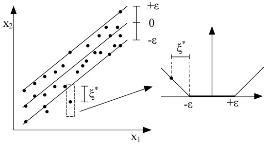
Figure 1.
Tolerable bandwidth of Support Vector Machine (SVM).
However, it is possible that no one linear regression function will satisfy the objective function in Equation (1) for all data and . Thus, the slack variables and are introduced for and , respectively; this allows regression errors to exist up to the value of and , but the objective function to remain satisfied, as shown in Figure 2. The slack variables and are defined by Equations (2) and (3):
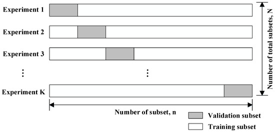
Figure 2.
K-fold cross validation.
Therefore, the objective function Equation (1) can be transformed to Equation (4), taking account of Equations (2) and (3):
and subject to
where the constant is a positive numerical value used to control the penalty for the observation lying outside the tolerable bandwidth, to prevent over-fitting. The value of determines the trade-off between the complexity of and the amount up to which deviations larger than ε are tolerated. A Lagrange function is then determined by introducing non-negative multipliers and for each observation as shown in Equation (5):
subject to
where is also known as the kernel function , which can be represented as polynomials, sigmoid kernels, radial basis function (RBF), and so on. The present study’s model adopted the RBF kernel, as shown in Equation (6). The RBF kernel maps samples nonlinearly from low-dimensional space into a higher-dimensional space. Therefore, it can deal with situations in which the relationships between input and output variables are nonlinear.
Obtaining the optimal solutions for Equation (5) requires using the three constraints shown in Equation (7), which indicates that all observations that are strictly within the tolerable bandwidth have Lagrange multipliers of and . Observations with non-zero Lagrange multipliers are called support vectors.
3.1.2. Model Training and Testing
For the proposed SVM model, a total dataset includes a training-sample dataset and a testing dataset . The former is used to construct the SVM prediction model and the latter to be tested to evaluate the accuracy of the prediction model. The effectiveness of the SVM model depends not only on its creator’s chosen learning algorithm but also on the required size of . Traditionally, is divided into and randomly, due to a lack of rigorous standards for such division. However, random division has some drawbacks: for example, and must be resampled until limitations on model-prediction accuracy are satisfied, in case the model-prediction error obtained by testing is excessive. This process of random resampling can be time-consuming. Accordingly, several cross-validation approaches to model-error evaluation have been introduced to help determine the optimal division of into and datasets. These include re-substitution validation, hold-out validation, leave-one-out cross-validation, and K-fold cross-validation (KFCV) [30]. The present study adopted KFCV, which divides equally into K subsets (K < ), and each K subset into one K-1 training dataset and one validation dataset, as shown in Figure 2. K experiments are then conducted, and the accuracy of any one such experiment is calculated using Equation (8):
where is the predicted value; is the target value; is the number of data in a validation subset, which is equal to , as shown in Figure 2; and is the mean absolute percent error (MAPE). Proposed by Lewis [31], MAPE has been widely used in the field of DM as a criterion to assess the performance of a model’s prediction-capability [32,33,34]. The predictions corresponding to different values of are listed in Table 1. In the case of , , , and , the prediction-capability of the model is defined as precise, good, reasonable and poor prediction, respectively. The experiment with the highest is set as the optimal model for further testing of new data.

Table 1.
Accuracy assessment criteria.
3.2. Development of Capacity Curves of Buildings
3.2.1. Pushover Analysis and the Capacity Spectrum Method
ATC-40 [35] recommends that buildings’ capacity curves be obtained by conducting pushover analysis, and defines seven damage states of structural elements, as shown in Figure 3. These are: B (yield point), IO (immediate occupancy), LS (life safety), CP (collapse prevention), C (ultimate strength), D (residual stress point), and E (final failure point), as shown in Figure 3b. In the present study, an ideal capacity curve of a building is conceptualized as an equivalent bilinear curve that covers an equal area as calculated up to the point of the first 20% drop in strength along the ideal pushover curve [36]. As such, an equivalent capacity curve can be depicted using points: yield and ultimate strengths and the force-displacement relation connecting these points are then converted into a spectral acceleration-displacement relation [35], and , as shown in Figure 3c, to facilitate direct comparison with the seismic-demand spectrum curve. As noted above, the intersection of the equivalent capacity curve and the seismic-demand curve marks a building’s performance point, i.e., the maximum displacement it can withstand under the seismic-demand curve in question. As such, the damage states of each structural element of the building can be determined. As shown in Figure 3a, for example, the finite element model of a building is built in SAP2000 and then the static pushover analysis is carried out to generate the building’s capacity curve. At the performance point, there are 341 structural elements are subjected to elastic deformation (A-B); 149 elements subjected to B-IO; 144 elements subjected to IO-LS, and so on.
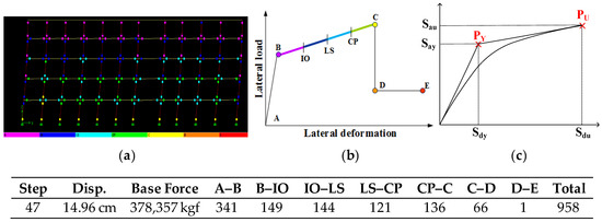
Figure 3.
(a) Damage states of structural components at the ultimate point ; (b) Deformation-load relation of a structural component; (c) Capacity curve.
3.2.2. Selection of Building Characteristics
FEMA154 [14] sets forth three principles to guide the selection of building characteristics appropriate for use in evaluations of the vulnerability of existing buildings. These are: simplicity/manageable numbers; visual accessibility by surveyors; and representativeness of vulnerability. In light of these principles, the present methodology adopted 20 building characteristics (Table 2) that were previously identified as relevant to seismic vulnerability [18,25,37]. For example, building stories can reflect the building’s functional frequency; built years can represent the quality of materials with the assumption that the same building materials were used in the same built year; the total section area of vertical elements can reflect the lateral stiffness of a building; factor 15 to factor 18 are structural defects which can increase building’s seismic vulnerability [25].
Table 2.
Building characteristics.
FEMA154 [14] suggests that it should be possible to complete a survey of 20 such characteristics of one building within 30 min. Moreover, some characteristics—such as a building’s height, year built, or structural system—may also be easily obtainable from public census statistics databases or tax documents.
4. Model Verification
As briefly noted above, our first and second case studies that were conducted to illustrate the application of proposed SVM models utilized different, overlapping sets of building characteristics, numbering 11 and 20, respectively, for the assessment of buildings’ capacity curves. The 11 characteristics, from factor 1 to factor 11, are selected from the 20 factors mainly for two reasons. First, either factor 1 to factor 3 or factor 12 to factor 14 can reflect the contribution of columns to a building’s lateral stiffness; therefore, only factor 1 to factor 3 are used in the case with 11 characteristics. Second, the data of factor 1 to factor 11 are easy to be collected without special requirement on surveyors’ expertise, while the data collection of factor 15 to factor 20 largely relies on the expertise of surveyors regarding structural engineering.
The buildings in question were drawn from the previously mentioned NCREE database of more than 5400 Taiwanese schools, which for each building includes all 20 of the characteristics noted in Table 2, and a capacity curve ( and . For verification of the proposed SVM models, we used our sets of 11 and 20 building characteristics as the inputs, and spectral-yield displacement , spectral-yield acceleration , spectral ultimate displacement , and spectral ultimate acceleration as the four outputs. The proposed model set and tested 11 training datasets ranging in size from 400 to 4,400 samples, in intervals of 400. The tests are performed on an Intel® CoreTM i7-6700 CPU@ 3.4GHz with 24 GB RAM in the environment of Microsoft Windows 10.
The computational time for each experiment is shown in Table 3. The total computational time is 4077 s (68 min). The computational time increases slightly as the number of building characteristics increases, while it increases significantly as the number of training data increases. In the first case study, for example, as the number of training data increased by 10 times, from 400 to 4400, the computational time increased by 88 times, from 5 s to 445 s.
Table 3.
The computational time for each experiment(s).
The present study adopted 10-fold cross validation (K = 10) as recommended by Chen et al.’s study [18] for all 11 sizes of training dataset. Table 3 presents the average validation accuracies of each experiment obtained via Equation (8) and 10-fold cross-validation for the proposed model with a training dataset of 4400 samples. Specifically, with 11 building characteristics as the inputs for and , these average validation accuracies were 0.666 and 0.648, respectively; and with 20 building characteristics as the inputs for and , they were 0.709 and 0.695, respectively. As noted in Table 1, such validation accuracies indicate that both the 11-characteristic and 20-characteristic models are reasonably accurate at predicting and when 4400 training samples are used. The experiment with the highest validation accuracies out of all 10 experiments, which are those ones with the maximum values in validation accuracies in Table 4, was selected as the optimal model for further model testing. Finally, for the sake of maximum predictive accuracy, as recommended by Riedel et al.’s study [26], the present study adopted a proportion of 5:1 between the sizes of the training dataset and the testing dataset.
Table 4.
Accuracy of 10-fold cross validation (training sample size of 4400).
In the first case study, the first 11 building characteristics in Table 2 were used as the model inputs, and and as outputs. First, we tested the influence of all 11 sizes of training dataset on the model’s prediction accuracy (Table 4), with 30 trials run for each training size using samples randomly selected from among the NCREE’s 5400 buildings. The resulting accuracies of the output are presented in Figure 4 and Table 5, which show that such accuracies increased slightly as the size of the training dataset increased: from 0.51 with a training dataset of 400 samples, to 0.54 at 4400 samples. This implies that when only 11 building characteristics were used as model inputs, the proposed SVM model could only achieve an accuracy of 0.52 in the prediction of , even when its training sample was as large as 4400; and that improvements in accuracy based solely on further increases in the size of the training dataset (as opposed to the number of building characteristics) are unlikely to be dramatic.
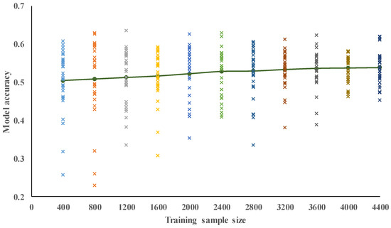
Figure 4.
Model accuracy for spectral-yield displacement with 11 building characteristics.
Table 5.
Model accuracy with testing 11 building characteristics for spectral-yield displacement .
We also observed that the standard deviation (SD) of our SVM models’ prediction accuracy over 30 trials decreased as the size of the training dataset increased: from 0.12 with a training dataset size of 400 is 0.12, to 0.04 at a size of 4400 samples, with a maximum value of 0.63 and a minimum of 0.03 (Table 5). These results indicate that the reliability of the proposed model can be increased by enlarging the training dataset, at least up to a point. As can be seen from Figure 5, which shows the relationship between the predicted and target values of in the 11-building-characteristic case with a sample size of 4400. From Table 6 and Figure 6 and Figure 7, all the above discussions regarding the results of output apply broadly to , , and .
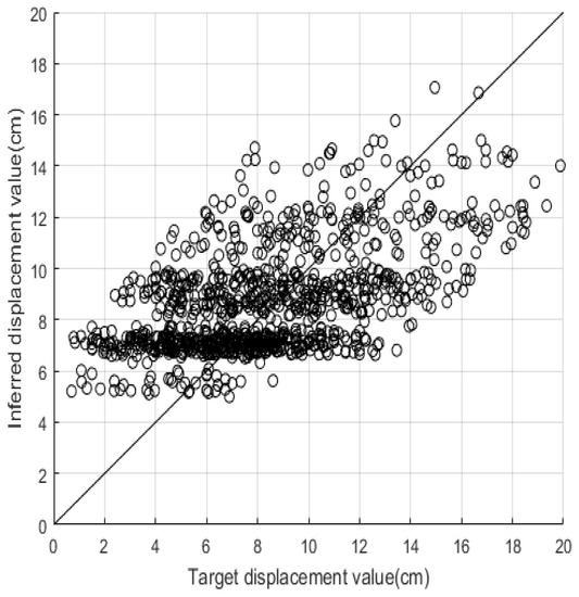
Figure 5.
Test results of 4400 training samples for spectral-yield displacement with 11 building characteristics.
Table 6.
Model accuracy with testing 11 building characteristics for spectral-yield acceleration .
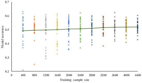
Figure 6.
Model accuracy for spectral-yield displacement with 11 building characteristics.
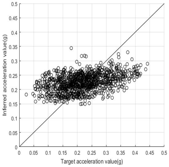
Figure 7.
Test results of 4400 training samples for spectral-yield displacement with 11 building characteristics.
In the second case study, which used all 20 of the building characteristics in Table 2 as model inputs, we also tested the influence of all 11 training-dataset sizes on prediction accuracy, again running 30 trials for each training-dataset size using samples randomly selected from the NCREE’s buildings. The output results are shown in Table 7 and Figure 8, where we can observe that the average values of model accuracy increase along with the size of the training dataset: from 0.64 at 400 samples, to 0.74 at 4400. In other words, when our selected 20 building characteristics are used as the inputs, our SVM model can achieve an average accuracy of 64% in the prediction of buildings’ seismic vulnerability using a relatively small training dataset of 400, but its average accuracy increased to 74% if the training-dataset size is increased to 4400: i.e., a 42% improvement over the 11-building-characteristic model with a dataset of the same (largest) size.
Table 7.
Model accuracy with testing 20 building characteristics for spectral-yield displacement .
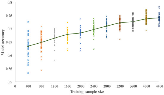
Figure 8.
Model accuracy for spectral-yield displacement with 20 building characteristics.
We again observed that the SD of model accuracy across the 30 trials decreased along with the size of the training dataset: from 0.04 at 400 to 0.02 at 4400, as shown in Table 6. In contrast to the results of the first case study, where the SDs for accuracy at sample sizes of 400 and 4400 were 0.12 and 0.04, respectively, such SDs in the second case study were limited in range to between 0.04 and 0.02, and converged at 0.02 if the size of the training dataset was greater than 1600 or more. These results indicate that the proposed SVM model can achieve high reliability of accuracy if all 20 building characteristics are used as its inputs, even using a relatively small training dataset of 400. Figure 9 illustrates the relationship between the predicted and target results of in the 20-building-characteristic case with a training dataset of 4400 and a model accuracy of 0.74. As compared with the equivalent figure for the first case study (Figure 5), we can observe less dispersion of the predicted values, with more falling within the tolerable bandwidth of the proposed model. All of our previous comments regarding the results for output can also be applied to (as shown in Table 8 and Figure 10 and Figure 11), as well as to and .
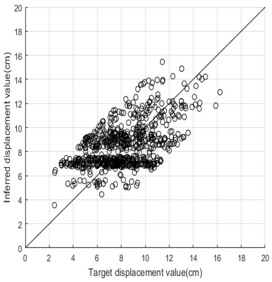
Figure 9.
Test results of 4400 training samples for spectral-yield displacement with 20 building characteristics.
Table 8.
Model accuracy with testing 20 building characteristics for spectral-yield acceleration .
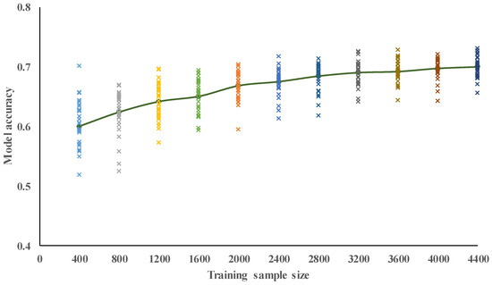
Figure 10.
Model accuracy for spectral-yield displacement with 20 building characteristics.
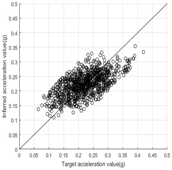
Figure 11.
Test results of 4400 training samples for spectral-yield displacement with 20 building characteristics.
5. Discussion and Conclusions
The negative impact of an earthquake on a building is primarily conceptualized as a function of its seismic vulnerability. This vulnerability is generally analyzed via computational simulation models of seismic response, such as push-over analysis. Although push-over analysis can provide sophisticated information about a building’s seismic vulnerability in terms of a capacity curve, it is time-consuming, requiring an immense quantity and high quality of data on building characteristics; and precisely because of this extraordinary level of detail, it must be repeated on a building-by-building basis thousands of times when such computational analysis is applied at a regional scale. It was primarily for this reason that the present study developed an SVM model for rapidly assessing buildings’ seismic vulnerability at the macroscale, in terms of spectral yield and ultimate points of their capacity curves, and .
In each of our two case studies, one with 11 and the other with 20 building characteristics, 11 different sizes of training dataset ranging from 400 to 4400 samples were tested. In the first case, the results for output indicate that, with only 11 building characteristics as inputs, the proposed SVM model could only achieve 52% prediction accuracy, even at the largest size of training dataset. In the second case study, taking the output as an example, model accuracy reached 64% with a training-dataset size of just 400, and improved to 74% at a size of 4400; and parallel results were obtained for , and . Importantly, our results imply that high reliability of prediction accuracy of the proposed model can be achieved if all 20 building characteristics are used as model inputs, regardless the size of training dataset, at least within the 400–4400 range that we studied. Additionally, comparing the first case study with the second case study, increasing training data can only slightly improve the prediction accuracy of models in the first case study, while increasing training data can significantly increase the prediction accuracy of models in the second case study, and such increasing trend seems to be continuous as the training dataset becomes larger. Such results indicate that the SVM model in the first case study could be underfitting, which means the number of building characteristics are too less to obtain high prediction accuracy even with a large training dataset. On the other hand, with more building characteristics, the prediction accuracy of the models in the second case study is expected to be improved with more training data.
In short, the above case studies, and particularly the second one, confirm the effectiveness and reliability of our proposed new data-mining technique (SVM) for rapid, regional-scale assessment of buildings’ seismic vulnerability in terms of their capacity curves. Coupled with seismic-demand curves, a seismic risk assessment of the buildings at a regional scale can also be done rapidly by determining their performance points using their capacity curves obtained by our proposed SVM model. As well as obviating the need to construct far more complex computational models for the same purpose, our technique could readily be extended to regional-scale estimation of other natural disaster risks to buildings, such as high winds and floods.
Author Contributions
Conceptualization, Z.Z., and T.-Y.H.; Methodology, Z.Z. and H.-H.W., and J.-H.C.; Validation, Z.Z. and H.-H.W.; Resources, T.-Y.H.; Data curation, Z.Z., H.-H.W., and T.-Y.H.; Writing—original draft preparation, Z.Z. and H.-H.W.; writing—review and editing, H.-H.W. and J.-H.C.
Funding
This research received no external funding.
Conflicts of Interest
The authors declare no conflict of interest.
References
- Kircher, C.A.; Whitman, R.V.; Holmes, W.T. HAZUS earthquake loss estimation methods. Nat. Hazards Rev. 2006, 7, 45–59. [Google Scholar] [CrossRef]
- Grossi, P.; Kunreuther, H.; Patel, C.C. Catastrophe Modeling: A New Approach to Managing Risk; Springer: Boston, MA, USA, 2005. [Google Scholar]
- Mahsuli, M.; Rahimi, H.; Bakhshi, A. Probabilistic seismic hazard analysis of Iran using reliability methods. Bull. Earthq. Eng. 2019, 17, 1117–1143. [Google Scholar] [CrossRef]
- Deligiannakis, G.; Papanikolaou, I.; Roberts, G. Fault specific GIS based seismic hazard maps for the Attica region, Greece. Geomorphology 2018, 306, 264–282. [Google Scholar] [CrossRef]
- Ahmad, R.A.; Singh, R.P.; Adris, A. Seismic hazard assessment of Syria using seismicity, DEM, slope, active faults and GIS. Remote Sens. Appl. Soc. Environ. 2017, 6, 59–70. [Google Scholar] [CrossRef]
- Ferreira, T.M.; Vicente, R.; Da Silva, J.M.; Varum, H.; Costa, A. Seismic vulnerability assessment of historical urban centres: case study of the old city centre in Seixal, Portugal. Bull. Earthq. Eng. 2013, 11, 1753–1773. [Google Scholar] [CrossRef]
- Maio, R.; Ferreira, T.M.; Vicente, R.; Estêvão, J. Seismic vulnerability assessment of historical urban centres: Case study of the old city centre of Faro, Portugal. J. Risk Res. 2016, 19, 551–580. [Google Scholar] [CrossRef]
- Maio, R.; Ferreira, T.M.; Vicente, R. A critical discussion on the earthquake risk mitigation of urban cultural heritage assets. Int. J. Disaster Risk Reduct. 2018, 27, 239–247. [Google Scholar] [CrossRef]
- Cannizzaro, F.; Pantò, B.; Lepidi, M.; Caddemi, S.; Caliò, I. Multi-directional seismic assessment of historical masonry buildings by means of macro-element modelling: Application to a building damaged during the L’Aquila earthquake (Italy). Buildings 2017, 7, 106. [Google Scholar] [CrossRef]
- Fagundes, C.; Bento, R.; Cattari, S. On the seismic response of buildings in aggregate: Analysis of a typical masonry building from Azores. In Structures; Elsevier: Amsterdam, The Netherlands, 2017; pp. 184–196. [Google Scholar]
- Casapulla, C.; Argiento, L.U.; Maione, A. Seismic safety assessment of a masonry building according to Italian Guidelines on Cultural Heritage: simplified mechanical-based approach and pushover analysis. Bull. Earthq. Eng. 2018, 16, 2809–2837. [Google Scholar] [CrossRef]
- Greco, A.; Lombardo, G.; Pantò, B.; Famà, A. Seismic Vulnerability of Historical Masonry Aggregate Buildings in Oriental Sicily. Int. J. Archit. Herit. 2018, 1–24. [Google Scholar] [CrossRef]
- Kircher, C.A.; Nassar, A.A.; Kustu, O.; Holmes, W.T. Development of building damage functions for earthquake loss estimation. Earthq. Spectra 1997, 13, 663–682. [Google Scholar] [CrossRef]
- FEMA. FEMA154 Rapid Visual Screening of Buildings for Potential Seismic Hazards: A Handbook; Federal Emergency Management Agency: Washington, DC, USA, 2002.
- Guéguen, P.; Michel, C.; LeCorre, L. A simplified approach for vulnerability assessment in moderate-to-low seismic hazard regions: application to Grenoble (France). Bull. Earthq. Eng. 2007, 5, 467–490. [Google Scholar] [CrossRef]
- Milutinovic, Z.V.; Trendafiloski, G.S. Risk-UE An advanced approach to earthquake risk scenarios with applications to different european towns. In Contract: EVK4-CT-2000-00014, WP4: Vulnerability of Current Buildings; European Commission: Brussels, Belgium, 2003. [Google Scholar]
- Mansour, A.K.; Romdhane, N.B.; Boukadi, N. An inventory of buildings in the city of Tunis and an assessment of their vulnerability. Bull. Earthq. Eng. 2013, 11, 1563–1583. [Google Scholar] [CrossRef]
- Chen, C.-S.; Cheng, M.-Y.; Wu, Y.-W. Seismic assessment of school buildings in Taiwan using the evolutionary support vector machine inference system. Expert Syst. Appl. 2012, 39, 4102–4110. [Google Scholar] [CrossRef]
- Nakhaeizadeh, G.; Taylor, C. Machine learning and statistics. Stat. Comput. 1998, 8, 89. [Google Scholar]
- Yao, X.; Tham, L.; Dai, F. Landslide susceptibility mapping based on support vector machine: A case study on natural slopes of Hong Kong, China. Geomorphology 2008, 101, 572–582. [Google Scholar] [CrossRef]
- Lin, G.-F.; Chou, Y.-C.; Wu, M.-C. Typhoon flood forecasting using integrated two-stage support vector machine approach. J. Hydrol. 2013, 486, 334–342. [Google Scholar] [CrossRef]
- Lin, J.-Y.; Cheng, C.-T.; Chau, K.-W. Using support vector machines for long-term discharge prediction. Hydrol. Sci. J. 2006, 51, 599–612. [Google Scholar] [CrossRef]
- Tripathi, S.; Srinivas, V.; Nanjundiah, R.S. Downscaling of precipitation for climate change scenarios: A support vector machine approach. J. Hydrol. 2006, 330, 621–640. [Google Scholar] [CrossRef]
- Kao, W.-K.; Chen, H.-M.; Chou, J.-S. Aseismic ability estimation of school building using predictive data mining models. Expert Syst. Appl. 2011, 38, 10252–10263. [Google Scholar] [CrossRef]
- Chen, H.-M.; Kao, W.-K.; Tsai, H.-C. Genetic programming for predicting aseismic abilities of school buildings. Eng. Appl. Artif. Intell. 2012, 25, 1103–1113. [Google Scholar] [CrossRef]
- Riedel, I.; Guéguen, P.; Dalla Mura, M.; Pathier, E.; Leduc, T.; Chanussot, J. Seismic vulnerability assessment of urban environments in moderate-to-low seismic hazard regions using association rule learning and support vector machine methods. Nat. Hazards 2015, 76, 1111–1141. [Google Scholar] [CrossRef]
- Miranda, E.; Akkar, S. Generalized interstory drift spectrum. J. Struct. Eng. 2006, 132, 840–852. [Google Scholar] [CrossRef]
- Vapnik, V. The Nature of Statistical Learning Theory; Springer Science & Business Media: Berlin, Germany, 2013. [Google Scholar]
- Drucker, H.; Burges, C.J.; Kaufman, L.; Smola, A.J.; Vapnik, V. Support vector regression machines. In Proceedings of the Advances in Neural Information Processing Systems, Denver, CO, USA, 3–5 December 1996; pp. 155–161. [Google Scholar]
- Geisser, S. Predictive Inference; CRC Press: Boca Raton, FL, USA, 1993; Volume 55. [Google Scholar]
- Lewis, C.D. Industrial and Business Forecasting Methods: A Practical Guide to Exponential Smoothing and Curve Fitting; Butterworth-Heinemann: Oxford, UK, 1982. [Google Scholar]
- Pereira, F.C.; Rodrigues, F.; Ben-Akiva, M. Text analysis in incident duration prediction. Transp. Res. Part C Emerg. Technol. 2013, 37, 177–192. [Google Scholar] [CrossRef]
- Li, C.-S.; Chen, M.-C. A data mining based approach for travel time prediction in freeway with non-recurrent congestion. Neurocomputing 2014, 133, 74–83. [Google Scholar] [CrossRef]
- Benzer, S.; Benzer, R.; Günal, A.Ç. Artificial neural networks approach in length-weight relation of crayfish (Astacus leptodactylus Eschscholtz, 1823) in Eğirdir Lake, Isparta, Turkey. J. Coast. Life Med. 2017, 5, 330–335. [Google Scholar] [CrossRef]
- ATC. ATC40- Seismic Evaluation and Retrofit of Concrete Buildings; Applied Technology Council: Redwood City, CA, USA, 1996. [Google Scholar]
- Kappos, A.J.; Panagopoulos, G.; Panagiotopoulos, C.; Penelis, G. A hybrid method for the vulnerability assessment of R/C and URM buildings. Bull. Earthq. Eng. 2006, 4, 391–413. [Google Scholar] [CrossRef]
- Cheng, M.-Y.; Wu, Y.-W.; Syu, R.-F. Seismic Assessment of Bridge Diagnostic in Taiwan Using the Evolutionary Support Vector Machine Inference Model (ESIM). Appl. Artif. Intell. 2014, 28, 449–469. [Google Scholar] [CrossRef]


© 2019 by the authors. Licensee MDPI, Basel, Switzerland. This article is an open access article distributed under the terms and conditions of the Creative Commons Attribution (CC BY) license (http://creativecommons.org/licenses/by/4.0/).