Transient Numerical Simulation of Regenerative Systems with Waste Gas Recirculation Strategies in Glass Production Plant

Featured Application

The numerical approach is applied to the simulation of regenerative chambers for glass production plants without or with gas recirculation strategies to reduce the NOx emissions.

Abstract

The glass production industry has one of the highest energy consumption rates and environmental emission impacts with respect to the existing industrial sectors. Glass furnaces nowadays are conceived with regenerative systems to take advantage of the residual heat from the combustion exhausts in order to increase the thermal efficiency of the system. The exhaust gases are also used in innovative systems to reduce the NOx emissions in specifically designed gas recirculation systems tailored to the glass furnace. In this paper, a numerical model for the simulation of the regenerative chambers in both steady and unsteady conditions is presented. The option of gas recirculation is also included. Special attention has been focused on the radiative heat transfer from the recirculated gases using a gas emissivity model previously developed by the authors.

1. Introduction

Regenerative heat exchanger for heat recovery in glass production processes is a type of heat exchanger where the thermal energy is intermittently stored by a solid medium usually made by a matrix of high thermal capacity and high surface to volume ratio refractories bricks. In the charging phase, a hot flow releases heat to the medium; in the discharge phase, a cold flow receives heat from the medium. In 1816, Robert Stirling invented the first thermal regenerator as a part of his well known engine [1]. Since the Industrial Revolution, thermal regenerators have been used for heat recovery from waste gases discharged by industrial processes. In 1857, Sir C.W. Siemens developed a regenerative furnace [2] where a continuous heat recovery was accomplished by a couple of regenerator chambers (RC) made of refractory material. The Siemens regenerator furnace layout is still largely used in industrial sectors where high temperature waste heat is produced, as in the case of glass industry. 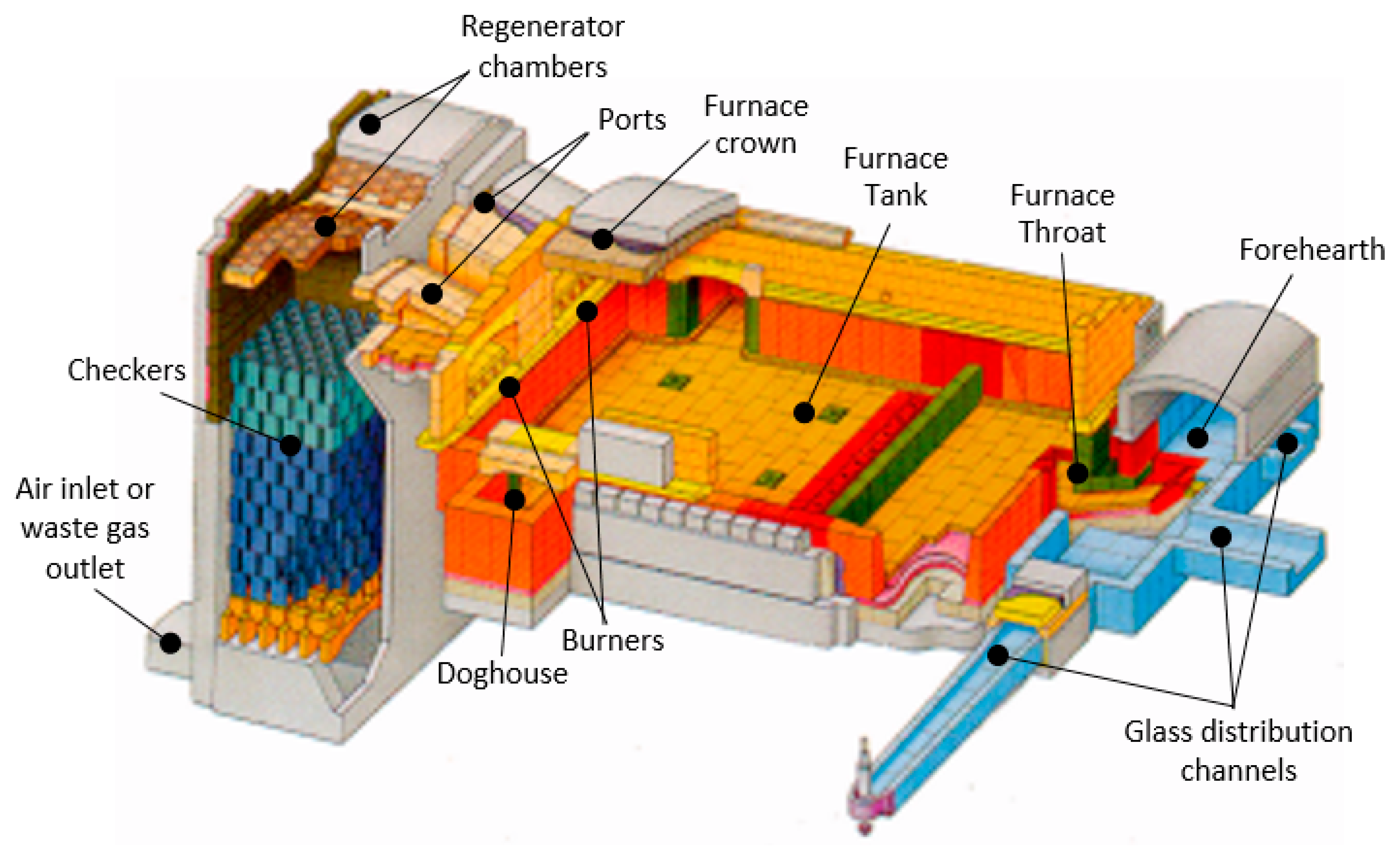Figure 1 shows the layout of a typical end-port (EP) glass furnace, a regenerative plant commonly used in the container glass production industry.

The raw material is heated and molten in a 1 to 1.5 m deep rectangular shaped tank. The glass pool is mainly heated by a flame in the combustion chamber (CC). Natural gas or heavy oil are used as fuel. The combustion process typically takes over the 90% of the energy input. Additional heat is frequently introduced by means of electrodes immersed into the glass with the purpose of increasing the convective flows into the glass bath. The raw material is introduced in the so-called “dog house” placed in the first part of the glass pool. The glass melts in the central part of the tank, and then it flows into a throat to be distributed to the channels that feed the forming machines. The glass bath is heated up to temperatures that can reach 1550 °C, and the exhaust gas leaves the CC at very high temperatures, over 1450 °C, corresponding to about 80–85% of the total energy consumption of the furnace. For this reason, the heat recovery of the waste gases is essential. Usually, heat regenerators are preferred over heat recuperators due to their higher conversion efficiency that significantly compensates the higher installation costs. In fact, a well-designed heat regenerator can easily recover 60% of the heat available from the exhaust gas, while a recuperator, due to the metallic materials involved, can recover up to 40% only.

The EP furnace has the typical regenerative furnace layout for a medium size plant. These two ports connect the CC to a couple of RCs—two large brick structures that contain perforated or cruciform brick stacks made of refractory material. The stack geometry produces internal ducts shaped to optimize the fluid to solid heat transfer.

The plant design is symmetrical. The combustion is fed alternatively from the preheated air by the left or the right RC. In the first phase, the air is preheated, flowing from the bottom to the top of the left RC, and it flows in the CC by the left port. The air is mixed with the fuel injected by the burners located under the port, creating a flame that covers about two thirds of the tank length. The exhaust gases come across the right ports in the right RC. Exhaust gases flow from the top to the bottom and release heat to the solid medium. A continuous combustion process and heat recovery is guaranteed by switching the cold and the hot flows into the two RCs.

Since 1930, there has been a significant scientific effort in the development of numerical models for the design of heat regenerators [3]. Hausen [4] published a mathematical model called the “ideal regenerator model” that uses differential equations to rigorously describe the heat transfer process in thermal regenerators. To overcome the mathematical difficulty of the rigorous model by Hausen, Rummel [5], in 1931, presented a simplified model called the “pseudo-recuperator model”, where the thermal regenerator at cyclic equilibrium is modeled as a conventional recuperator where fluid and solid temperatures are the time-mean temperatures in the real regenerator phases. Only 30 years later, Lambertson [6] and Willmott [7] published a solution of the “ideal regenerator model” differential equation system. Wilmott used the model to predict the regenerator performance under variable mass flow conditions [8] and to study the effects of the gas storage on the stack during the flow inversions [9]. In recent years, Sardeshpande et al. [10] and Tapasa et al. [11] developed simulation tools to investigate the energy performance of a regenerative glass furnace. Sardeshpande et al. [12] developed a model based on the Rummel’s hypothesis that is useful to analyze the regenerator performance under different operating conditions. The numerical solution of the Hausen’s model is currently no longer a limit. In [13], Sadrameli et al. developed a numerical model of a glass furnace regenerator based on the Hausen assumptions. Nowadays, heat regenerators can be efficiently simulated with state-of-the-art computational fluid dynamic (CFD) 3D techniques. Reboussin et al. [14] developed a CFD analysis to study the heat transfer in a glass furnace regenerator during the cold and the hot phases. In [15,16], the authors described a similar CFD procedure where a specific model for the heat transfer and pressure drop phenomena into the stacking is detailed. A lower order numerical model for the regenerator—under steady operation—was set up and validated using the results from high fidelity CFD [17]. CFD models have also been developed for the Strategic Waste Gas Recirculation (WGR) system [18]. It is a thermal regenerator add-on module developed within the PrimeGlass project framework [19]. The WGR system, developed to reduce NOx emissions, is a ventilation system that feeds, at its base, the RC operating in the cold phase with a fraction of the waste gas flow rate extracted from the base of the RC operating in the hot phase. A preliminary numerical model developed for steady analysis [17] has been extended with a model for gas thermal radiation [20] in order to predict the additional thermal effects in the air phase in the presence of CO-CO₂-H₂O molecules (due to the exhaust gases using a WGR system). In this paper, a lower order numerical approach for the unsteady analysis of the thermal regenerator, with or without the WGR system, is presented.

The model is firstly applied to predict the thermal performance of regenerators with different geometrical dimensions to demonstrate its applicability for design purposes. The model is then used to simulate the thermal effects of the WGR system.

The present lower order model is developed for the design and development of the regenerative system to set up and optimize the plant with the WGR solution. The transient analysis option gives an increased opportunity to setup the WGR system and to optimize the switch time between hot and cold phases. In fact, the heat transfer process is altered by the presence of the exhaust gases into the combustion air due to the increase of radiation. The present model with transient analysis is a first step in the development of a digital twin for the entire furnace system.

2. Simulation Model

The numerical transient model of the thermal regenerator is implemented using the software Matlab with the Simulink tool. As in the real system, the numerical model is composed of two RCs sub-models.

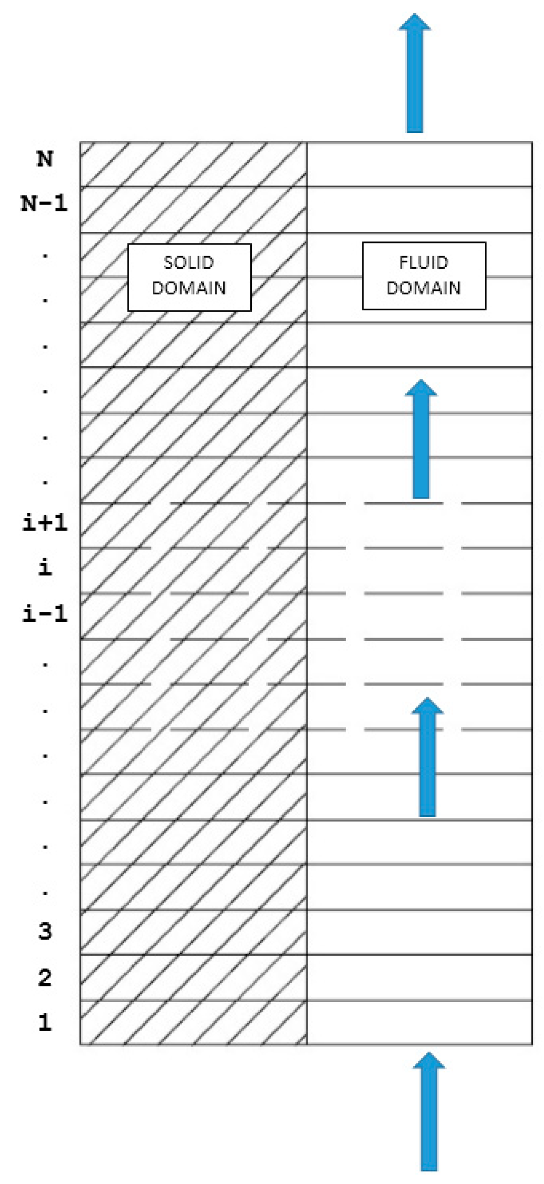
Each RC model is modeled with a solid domain representing the refractory and with a fluid domain that models the cold or the hot fluid phase. In order to reproduce the temperature profile, the solid and the fluid domains are discretized with N finite cells, as shown in Figure 2. For each cell, a transient energy balance equation is added to describe the heat and mass transfer between the adjacent cells using the following hypothesis:

• No heat transfer through the casing with the external environment,
• No seepage or flux leakage from the casing,
• Fluid thermal properties function of temperature only,
• Incompressible flow.

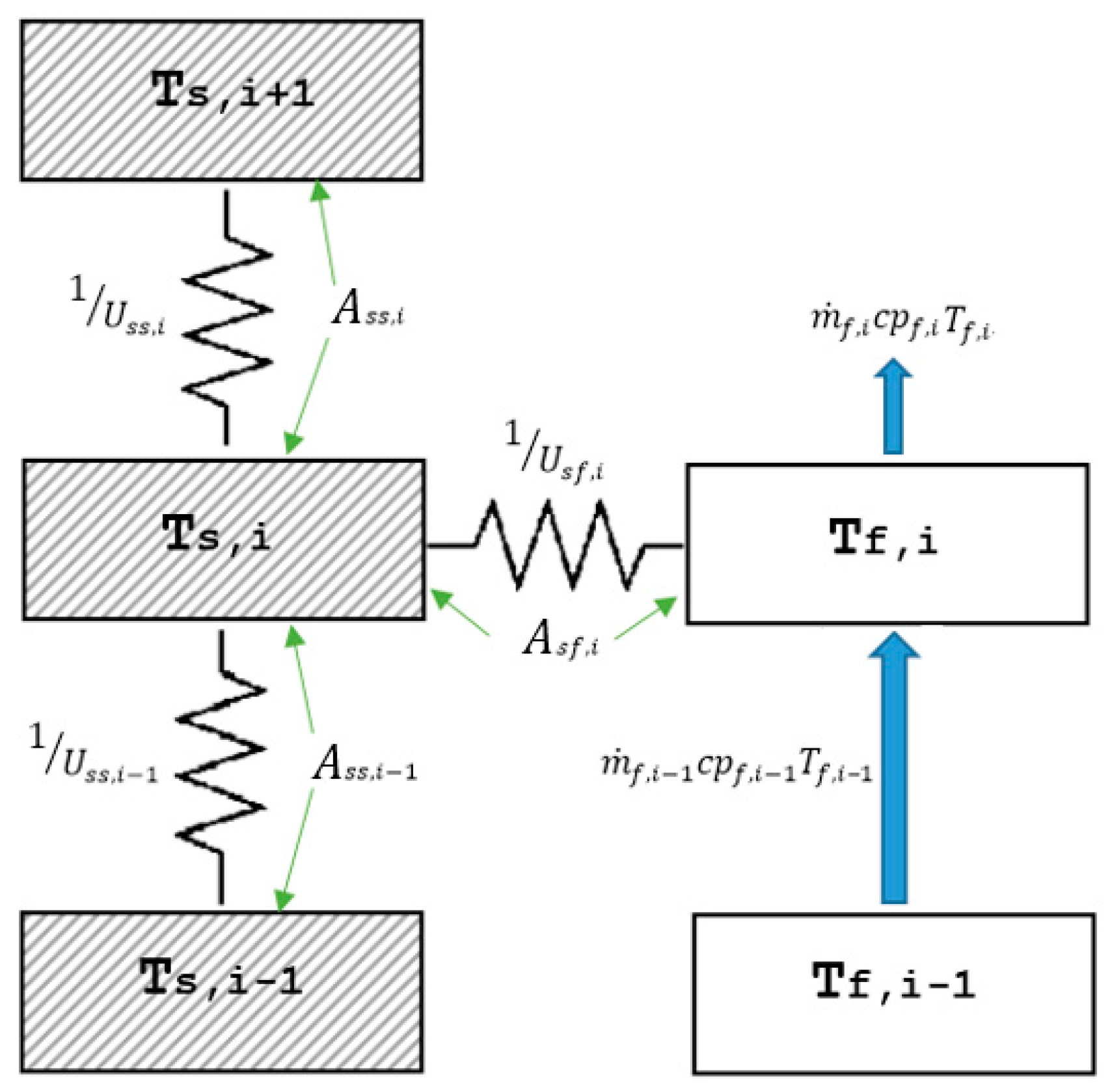
Figure 3 shows a sketch of the energy interaction between adjacent cells. The energy balance of the generic i^th fluid cell can be evaluated by Equation (1): the internal energy time variation (left side of the equation) is equal to the sum of the contributions of the heat exchanged with the adjacent solid cell and the net heat transported by the mass flow from the inlet to the outlet of the fluid cell.

The energy balance of the generic i^th solid cell can be evaluated by Equation (2): the internal energy time variation (left side of the equation) is equal to the sum of the contributions of the heat exchanged with the adjacent fluid cell and upper and lower solid cells.

$$\begin{array}{c}\mathrm{For}i=1,\cdots ,N\\ m_{f,i}c{v}_{f,i}\frac{{\dot{dT}}_{f,i}}{dt}={\dot{m}}_f\left(c{p}_{f,i-1}{T}_{f,i-1}-c{p}_{f,i}{T}_{f,i}\right)+\left(U_{sf,i}{A}_{sf,i}\right)\left(T_{s,i}-T_{f,i}\right)\end{array}$$

(1)

$$\begin{array}{c}{m}_{s,i}c{v}_{s,i}\frac{{\dot{dT}}_{s,i}}{dt}=\left(U_{ss,i-1}{A}_{ss,i-1}\right)\left(T_{s,i-1}-T_{s,i}\right)+\left(U_{ss,i+1}{A}_{ss,i+1}\right)\left(T_{s,i+1}-T_{s,i}\right)\\ +\left(U_{sf,i}{A}_{sf,i}\right)\left(T_{f,i}-T_{s,i}\right)\end{array}$$

(2)

where the subscript f and s refer to the fluid and solid domain, respectively, ${\dot{m}}_s$ is the cell mass, ${\dot{m}}_f$ is the mass flow, $cv$ and $cp$ are respectively the specific heat flow at constant volume and pressure. The parameters $A_{sf,i}$ and $A_{ss,i}$ are respectively the heat transfer surface at the solid/fluid interface and at the solid/solid interface of the i^th layer. $U_{sf,i}$ and $U_{ss,i}$ are respectively the thermal transmittances between the solid and the fluid cells and between the two solid cells, defined in the following Equations (3) and (4).

$$\begin{array}{c}\mathrm{For}i=1,\cdots ,N\\ U_{sf,i}=\frac{1}{\frac{1}{h_{tot,i}}+\frac{th}{k_s}}\left[\frac{\mathrm{W}}{{\mathrm{m}}^2·\mathrm{K}}\right]\end{array}$$

(3)

$$U_{ss,i}=\frac{k_s}{\raisebox{1ex}{$H$}\!\left/ \!\raisebox{-1ex}{$N$}\right.}\left[\frac{\mathrm{W}}{{\mathrm{m}}^2·\mathrm{K}}\right]$$

(4)

where $h_{tot}$ is the total heat transfer coefficient; it includes the convective and radiant effects between the gas flow and the checkers. $th$ is half of the refractories thickness, $k_s$ is its thermal conduction coefficient, and $H$ is the total checkers height.

The equation system described by Equations (1) and (2) can be re-arranged as in Equations (5) and (6).

$$\frac{d}{dt}\left[T_f\right]=\left[a_f\right]\left[T_f\right]+\left[b_f\right]\left[T_s\right]+\left[c_f\right]T_{f,ini}$$

(5)

$$\frac{d}{dt}\left[T_s\right]=\left[a_s\right]\left[T_s\right]+\left[b_s\right]\left[T_f\right]$$

(6)

where $\left[T_f\right]$ and $\left[T_s\right]$ are the fluid and solid temperature arrays (Equations (7) and (8)), and $T_{f,ini}$ is the fluid inlet temperature.

$$\left[T_f\right]=\left[T_{f,1},T_{f,2},\cdots ,T_{f,i},\cdots ,T_{f,N-1},T_{f,N}\right]$$

(7)

$$\left[T_s\right]=\left[T_{s,1},T_{s,2},\cdots ,T_{s,i},\cdots ,T_{s,N-1},T_{s,N}\right]$$

(8)

In the above equations $\left[a_f\right]$ and $\left[b_f\right]$ are squared matrices of order N with non-zero value and:

$$\begin{array}{c}\mathrm{For}i=1,\cdots ,N\\ a_{f,\left(i,i\right)}=\frac{-\left({\dot{m}}_{f}c{p}_{f,i}+U_{sf,i}{A}_{sf,i}\right)}{m_{f,i}c{v}_{f,i}}\end{array}$$

(9)

$$b_{f,\left(i,i\right)}=\frac{U_{sf,i}{A}_{sf,i}}{m_{f,i}c{v}_{f,i}}$$

(10)

$$\begin{array}{c}\mathrm{For}i=2,\cdots ,N\\ a_{f,\left(i,i-1\right)}=\frac{{\dot{m}}_{f}c{p}_{f,i}}{m_{f,i}c{v}_{f,i}}\end{array}$$

(11)

$\left[c_f\right]$ is an array with order N with a non-zero value at the first element:

$$c_{f,\left(1\right)}=\frac{{\dot{m}}_{f}c{p}_{f,i}}{m_{f,i}c{v}_{f,i}}$$

(12)

The terms $\left[a_s\right]$ and $\left[b_s\right]$ are squared matrices with order N with non-zero value in the following cells:

$$\begin{array}{c}\mathrm{For}i=1,\cdots ,N\\ a_{s,\left(i,i\right)}=\frac{-\left(U_{ss,i-1}{A}_{ss,i-1}+U_{sf,i}{A}_{sf,i}+U_{ss,i+1}{A}_{ss,i+1}\right)}{m_{s,i}c{v}_{s,i}}\end{array}$$

(13)

$$b_{s,\left(i,i\right)}=\frac{U_{sf,i}{A}_{sf,i}}{m_{s,i}c{v}_{s,i}}$$

(14)

$$\begin{array}{c}\mathrm{For}i=2,\cdots ,N\\ a_{s,\left(i,i-1\right)}=\frac{U_{ss,i-1}{A}_{ss,i-1}}{m_{s,i}c{v}_{s,i}}\end{array}$$

(15)

$$\begin{array}{c}\mathrm{For}i=1,\cdots ,N-1\\ a_{s,\left(i,i+1\right)}=\frac{U_{ss,i+1}{A}_{ss,i+1}}{m_{s,i}c{v}_{s,i}}\end{array}$$

(16)

2.1. Fluid Properties

The model is set up to simulate a flow mixture made by a combination of oxygen, nitrogen, carbon dioxide, and water vapor. For each regeneration phase, the mass concentration $w_j$ of each $j^{th}$ chemical element is given as reported in

Table 1. Air and exhaust gases chemicals mass concentration example.

		Air	Waste Gas
${\mathit{w}}_{\mathit{j}}\left[\raisebox{1ex}{${\mathbf{kg}}_{\mathbf{j}}$}\!\left/ \!\raisebox{-1ex}{${\mathbf{kg}}_{\mathbf{tot}}$}\right.\right]$	N2	0.791	0.687
	O2	0.209	0.023
	CO2	0	0.119
	H2O	0	0.171

. The mixture specific heat at constant pressure $c{p}_f$, is calculated as a weighted sum of the specific heats, as in Equation 17. The specific heat of each $j^{th}$ element is calculated using a 4^th degree polynomial function with two temperature ranges. The mixtures are considered ideal gases, i.e., the specific gas constant of the mixtures $R_f$ is a function of the chemical mass fraction and the molar mass $M{M}_j$, as in Equation (18). The fluids density ${\rho }_f$ can then be obtained using the equation of state for an ideal gas, as in Equation (19).

The fluid specific heat at constant volume $c{v}_f$ can be evaluated using the Mayer relation, as in Equation (20).

$$c{p}_f\left(T_f\right)=\sum w_{j}c{p}_j\left(T_f\right)\left[\frac{\mathrm{J}}{\mathrm{kg}·\mathrm{K}}\right]$$

(17)

$$R_f=8.314\ast \sum \raisebox{1ex}{$w_j$}\!\left/ \!\raisebox{-1ex}{$M{M}_j$}\right.\left[\frac{\mathrm{J}}{\mathrm{kg}·\mathrm{K}}\right]$$

(18)

$${\rho }_f\left(T_f\right)=\raisebox{1ex}{$p_{tot}$}\!\left/ \!\raisebox{-1ex}{$R_f{T}_f$}\right.\left[\raisebox{1ex}{$\mathrm{kg}$}\!\left/ \!\raisebox{-1ex}{${\mathrm{m}}^3$}\right.\right]$$

(19)

$$c{v}_f\left(T_f\right)=c{p}_f\left(T_f\right)-R_f\left[\frac{\mathrm{J}}{\mathrm{kg}·\mathrm{K}}\right]$$

(20)

The thermal properties of the solid domain, i.e., the refractories, are kept constant with temperature and along the regenerator height. It is assumed there exists a thermal conduction coefficient $k_s$ equal to 5 W/m²·K, a specific heat $c{v}_s$ equal to 1200 J/kg·K, and a density of 3500 kg/m³.

2.2. Geometrical Parameters

The following geometrical data for the regenerator are given:

• The total RC volume $V_{tot}$ and the fluid-volume fraction $F_f$.
• The total heat transfer surface between the fluid and the solid $A_{sf,tot}$.
• The hydraulic diameter $D_{ch}$ of the RC channels.
• The refractories average thickness $th$.

With these assumptions, the model geometrical parameters can be set:

$$A_{sf,i}=\raisebox{1ex}{$A_{sf,tot}$}\!\left/ \!\raisebox{-1ex}{$N$}\right.\left[{\mathrm{m}}^2\right]$$

(21)

$$V_{s,i}=\raisebox{1ex}{$\left(1-F_f\right)V_{tot}$}\!\left/ \!\raisebox{-1ex}{$N$}\right.\left[{\mathrm{m}}^3\right]$$

(22)

$$V_{f,i}=\raisebox{1ex}{$F_f\ast V_{tot}$}\!\left/ \!\raisebox{-1ex}{$N$}\right.\left[{\mathrm{m}}^3\right]$$

(23)

Finally, the mass of each cell is calculated from Equations (24) and (25).

$$m_{f,i}={\rho }_f\left(T_f\right)\ast V_{f,i}\left[\mathrm{kg}\right]$$

(24)

$$m_{s,i}={\rho }_s\ast V_{s,i}\left[\mathrm{kg}\right]$$

(25)

2.3. Heat Transfer Coefficients

The heat transfer characterization plays a crucial role in all heat exchanger modeling. The heat transfer in the RC is a complex phenomenon—the cold phase is characterized by a mixed forced-natural convection regime, whereas in the hot phase, the heat transfer is governed by the radiant heat emitted by the exhaust gases. In [15,16,17], the authors simulated the heat transfer in a single channel of an RC for a conventional glass plant, evaluating the total heat transfer coefficient across the RC height for cold or hot fluid phases. In [20], the attention was focused on a tool for the evaluation of the radiant gas emissivity crucial to study the WGR system strategies. The present lower order numerical model uses the values obtained in [17] for the heat transfer coefficients for the cold and the hot phases. In the case of the WGR system, the tool described in [20] is used for the evaluation of the radiant heat transfer coefficients to be implemented in the cold phase.

2.4. Simulation Model Setup

A real glass furnace regenerator is made by a couple of twin chambers, where the cold and hot flows are switched to maintain the thermal performance of the system. The alternate regenerator system is numerically modeled as a rotary regenerator with a non-continuous rotation.

The regenerator model couples two RC sub-models. The first RC, called Cold RC, simulates the cold phase fluid. The second RC, called Hot RC, simulates the hot phase fluid. The phase inversion between the RCs is modeled by switching, with a given timing, the temperature profile across the solid domain between the Cold and the Hot RC. Initial temperature profiles are set for the cold and the hot flows and for the solid domain. The mass flow rates, inlet temperature, and chemical composition are set to be constant in time. The model running in unsteady mode reaches the equilibrium after the simulation of about 100 to 200 phase inversions depending on the initial temperature conditions specified.

3. Applications to a Conventional Glass Thermal Regenerator

The regenerator model is applied to analyze the system performance with different size and operative conditions. As reported in [21], the performance of a periodic thermal storage can be evaluated using three non-dimensional parameters:

(1) The thermal efficiency ${\eta }_T$, i.e., the ratio between the air outlet and the exhaust gas inlet temperatures (Equation (26)):

$${\eta }_T=\raisebox{1ex}{$T_{air,out}$}\!\left/ \!\raisebox{-1ex}{$T_{exh,in}$}\right.$$

(26)

(2) The storage effectiveness $R$, i.e., the ratio between the energy absorbed by the air in a cycle and the energy available from the exhaust gas flow (Equation (27)):

$$R=\frac{{\dot{m}}_{air}c{p}_{air}{\tau }_{air}\left({\tilde{T}}_{air,out}-T_{air,in}\right)}{{\dot{m}}_{ex}c{p}_{ex}{\tau }_{ex}\left({\tilde{T}}_{ex,out}-T_{ex,in}\right)}$$

(27)

(3) The capacitance utilization $CU$, i.e., the ratio between the energy absorbed by the air in a cycle and the maximum energy that can be stored in the solid matrix (Equation (28)):

$$CU=\frac{{\dot{m}}_{air}c{p}_{air}{\tau }_{air}\left({\tilde{T}}_{air,out}-T_{air,in}\right)}{m_{s}c{v}_s\left(T_{exh,in}-T_{air,in}\right)}$$

(28)

In glass furnace regenerative systems, ${\eta }_T$ can commonly approach values close to one. This is possible due to the mass flow and specific heat imbalance between the air and the waste gas phases. From Equation (27), it is clear that if ${\eta }_T$ is equal to one, $R$ reaches its maximum value (Equation (29)). With this assumption, a specific effectiveness $\epsilon$ can be defined (Equation (30)) as the ratio between the actual storage effectiveness $R$ and $R_{max}$.

$$R_{max}=\raisebox{1ex}{${\dot{m}}_{air}c{p}_{air}$}\!\left/ \!\raisebox{-1ex}{${\dot{m}}_{exh}c{p}_{exh}$}\right.$$

(29)

$$\epsilon =\raisebox{1ex}{$R$}\!\left/ \!\raisebox{-1ex}{$R_{max}$}\right.$$

(30)

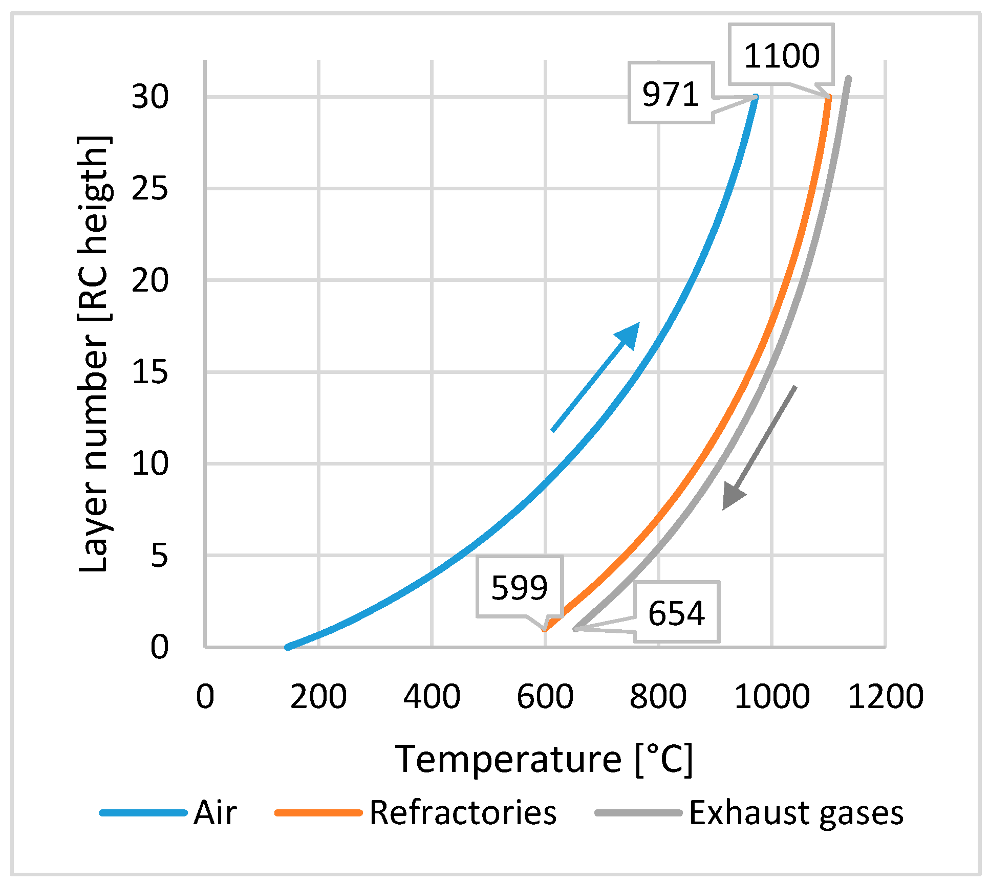
The analyses are performed with the following reference case: a thermal regenerator where each RC has a total volume of 100 m³, $F_f$ equal to 0.7, and a total heat transfer area equal to 2900 m². The regenerator is set up to work with a reverse time $\tau$ equal to 20 min.

The regenerator is fed with an exhaust mass flow rate equal to 4.88 kg/s at a temperature of 1135 °C and with an air mass flow rate equal to 3.77 kg/s at a temperature of 145 °C. The chemical composition of the air and exhaust gases are set as reported in Table 1. A constant linear profile of the heat exchange coefficients is set for each gas phase, as reported in [17]. Figure 4 shows the time-averaged temperature profile of the two flows and of the refractories. 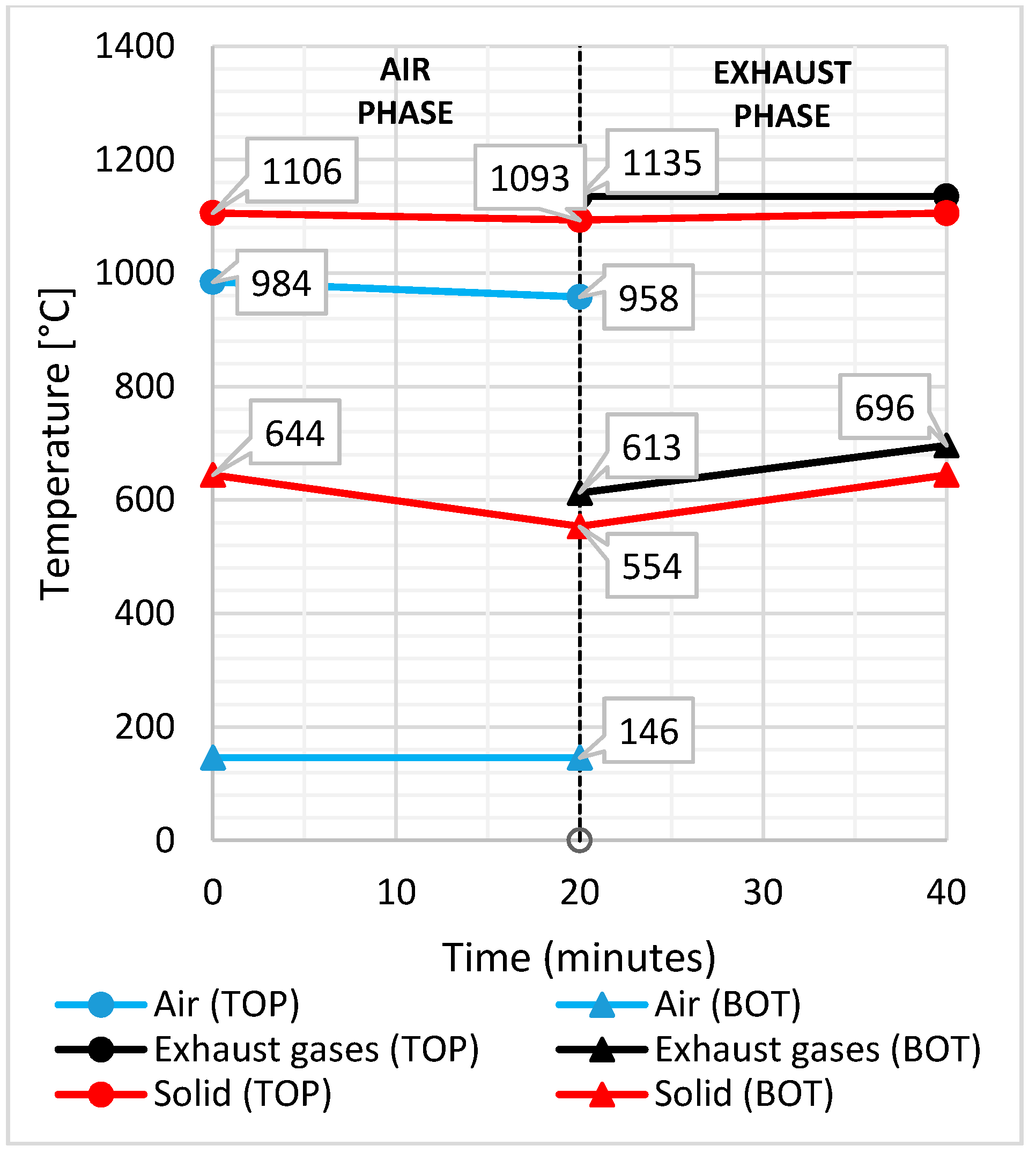Figure 5 shows the same variables on the top and the bottom layers of the RC over a regeneration cycle. From the above data, the ${\tilde{\eta }}_T$ is 0.883 with an oscillation of about 0.02 over the cycle, and the $R$ value is 0.482, which means $\epsilon$ equal to 0.834.

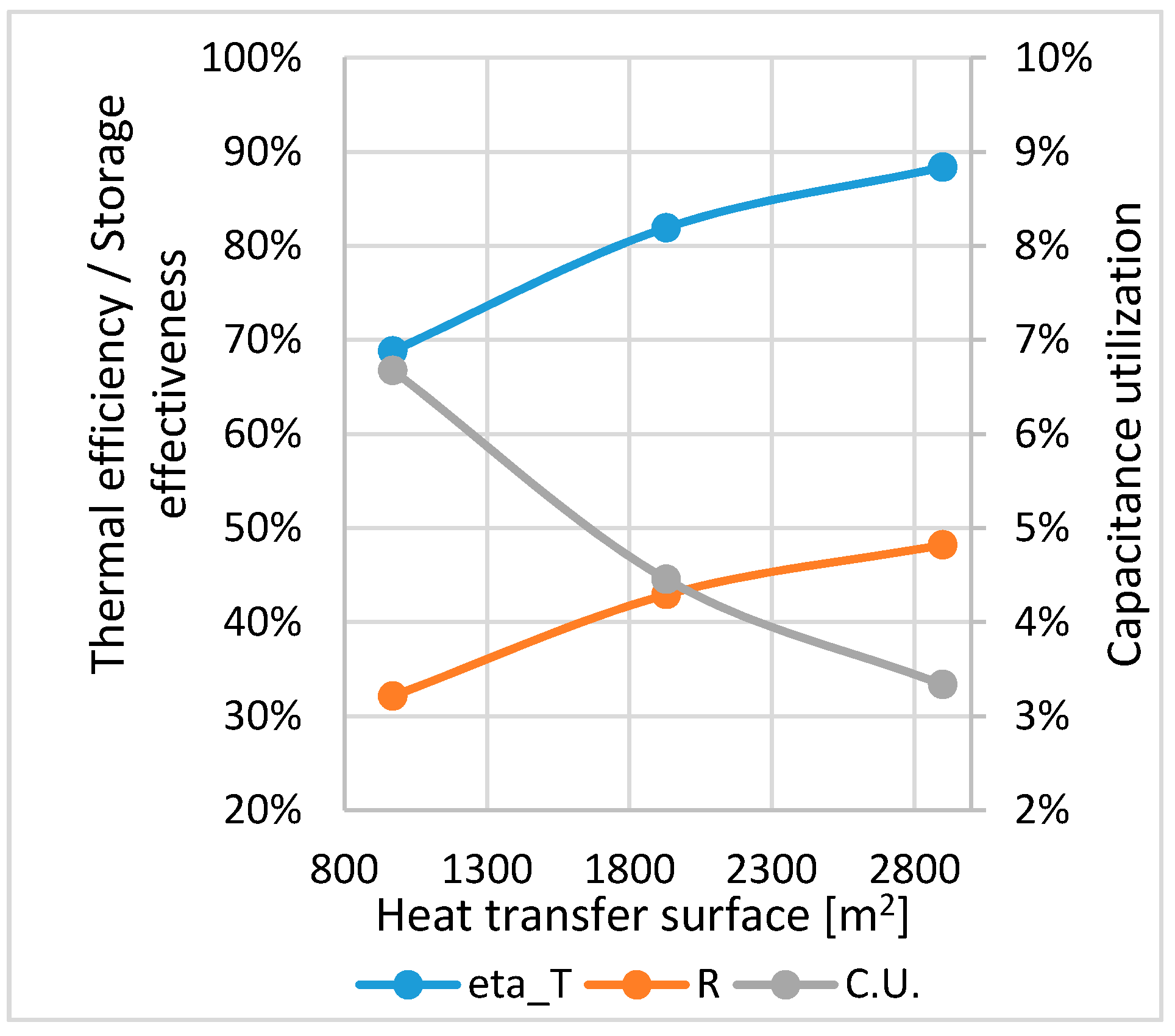
The unsteady regenerator model is then applied to compare three regenerative chambers of varying size, as detailed in

Table 2. Geometrical parameters of simulated cases.

	Case A	Case B	Case C
$A_{sf,tot}$	2900	1930	970	m2
$V_{tot}$	100	66.6	33.3	m3
$F_f$	0.7	0.7	0.7

. The heat transfer surface and the volume are gradually reduced. The inversion time equal to 20 min is kept. Figure 6 shows the value of the regenerative performance coefficients for each case. The ${\tilde{\eta }}_T$ increases with the RC size. The increase rate is more pronounced for changes in small RC. The $R$ shows a trend similar to ${\tilde{\eta }}_T$, and the $CU$ value decreases by increasing the RC volume. In fact, referring to Equation (28), the increase of the thermal capacity of the storage $m_{s}c{v}_s$ is more effective than the increase of the regenerator energy performance.

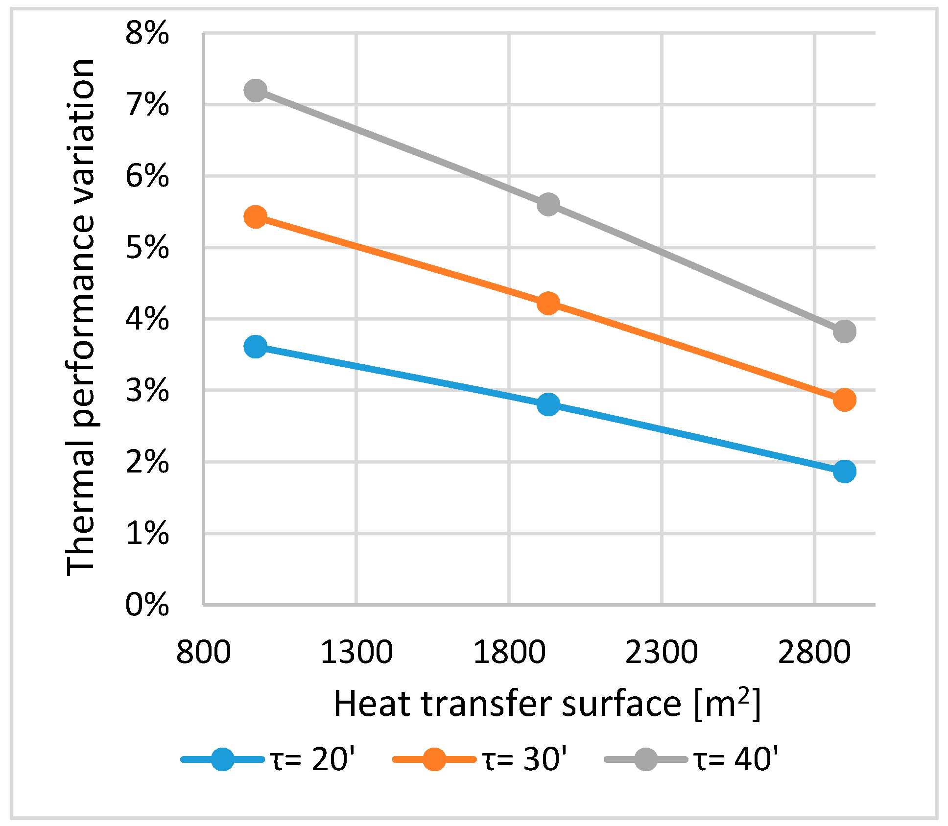
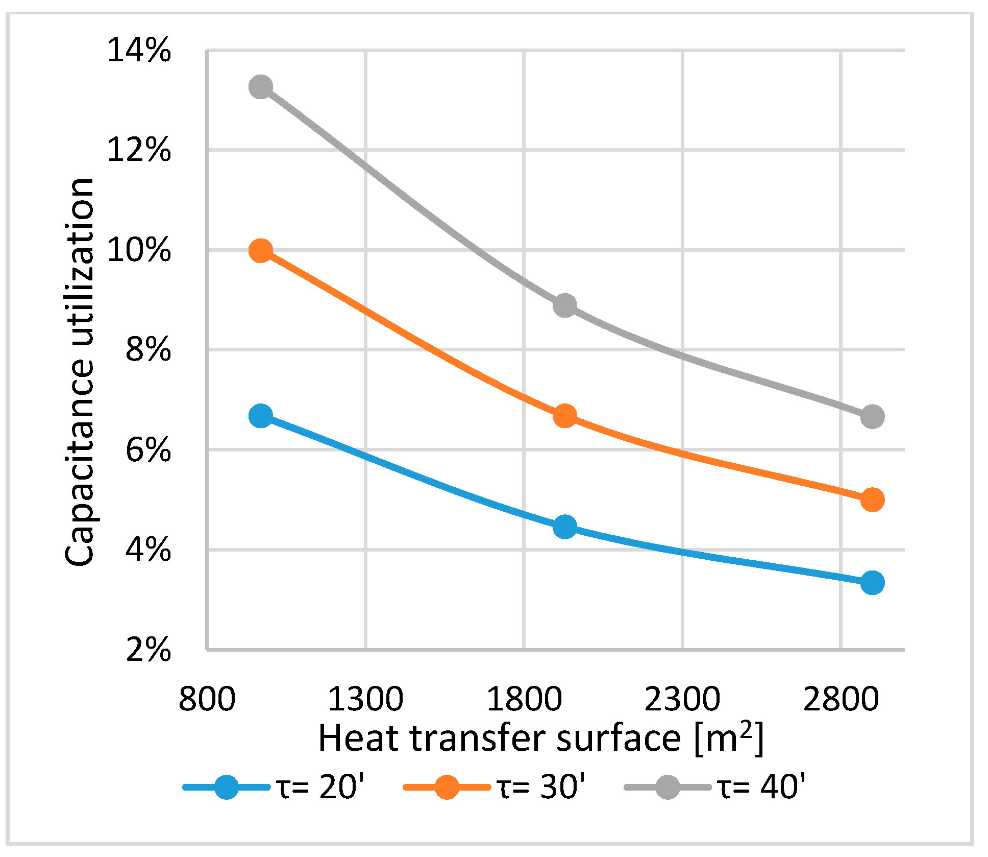
The model is then applied to the set of configurations from Table 2 by increasing the inversion time $\tau$: 20 - 30 - 40 min and the results are shown in Figure 7 and Figure 8. As before, with fixed RC geometry, the time-averaged outlet temperatures of the fluid ${\tilde{T}}_{air,out}$ and ${\tilde{T}}_{exh,out}$ are almost constant for the different $\tau$ values. The values of ${\tilde{\eta }}_T$, $R$, and $\epsilon$ do not change with $\tau$.

4. Model Application to Thermal Regenerator with WGR System

The unsteady regenerator model is applied to the analysis of the WGR system. The WGR system is a low NOx strategy where a portion of exhaust gas is recirculated at the base of the RC in the air phase. The experimental tests on pilot furnaces performed in the PrimeGlass project [19] have confirmed that the WGR system does have an impact on the thermal balance of the regenerative chambers due to the increase of the mass flow rate and the increase in heat exchange caused by the introduction of radiant chemical species into the combustion air.

In previous studies [16,18], the WGR system was studied using CFD models in order to optimize the distribution of the waste gas in the stacker and the port to CC of the Cold RC. The CFD domain included the complete 3D geometry of the Cold RC [17], and the WGR ports were added at the bottom of the chamber. Multiblock structured meshes were generated, and the CFD solutions were obtained using the Ansys CFX CFD platform. The CFD model solved the Reynolds Averaged Navier-Stokes (RANS) governing equations (continuity, momentum, energy) for the gas mixture using the second order upwind numerical scheme with the shear stress tensor (SST) turbulence closure added to model the effects of turbulence [15,16,17,18].

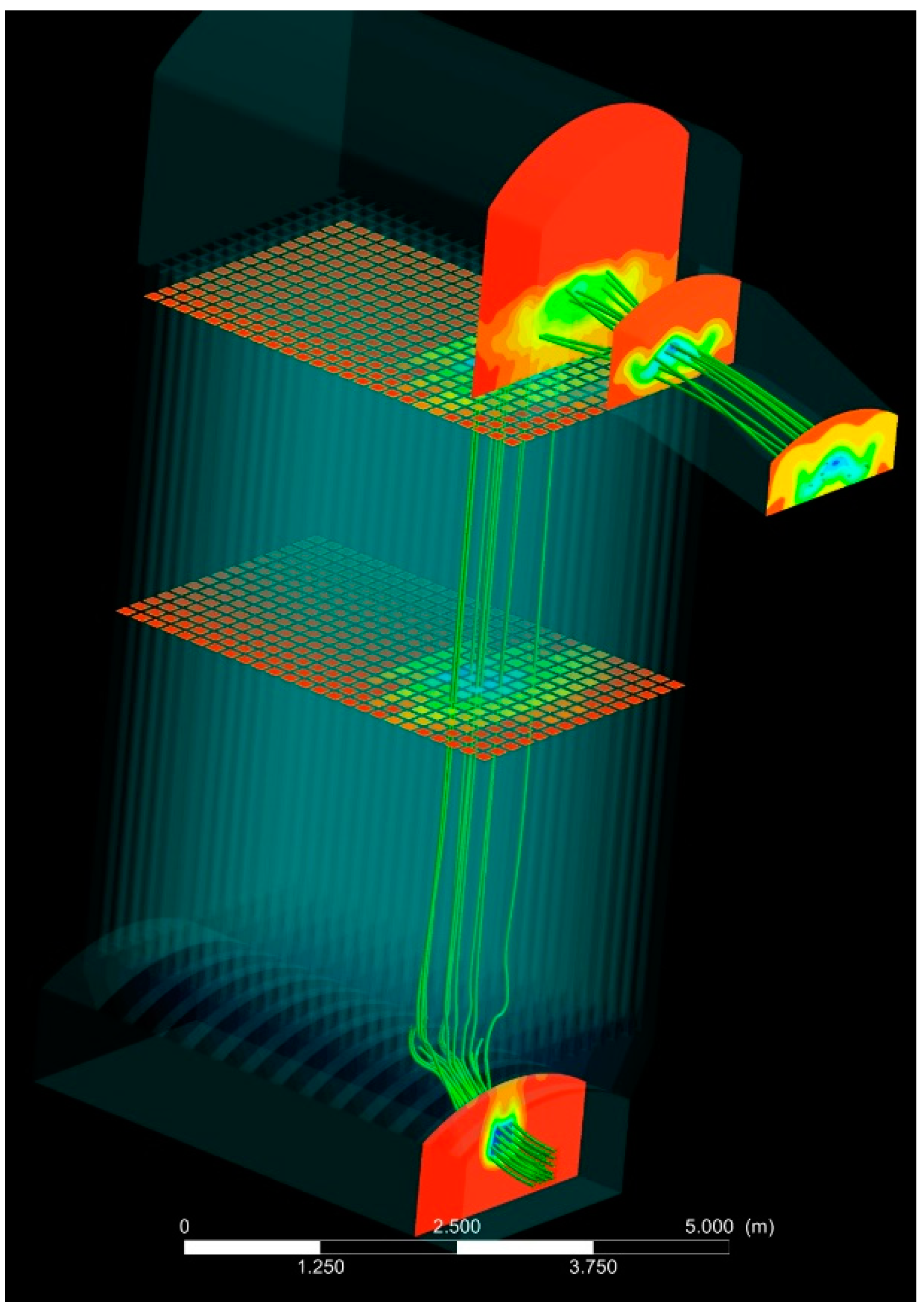
The WGR system is investigated using CFD by changing the waste gas mass flow rate and the layout of the inlet ports. The following typical post-processing of the CFD solution is performed to understand the WGR system performance. The numerical CFD results are post-processed in order to track the waste gas flow inside the RC by detecting of the O2 concentration. The resulting O2 patterns in the case of waste gas/air mass flow ratio of 20% are reported in Figure 9, Figure 10, and Figure 11. In Figure 9, the isosurface at 16% of oxygen concentration is highlighted in order to show the waste gas tracked across the Cold chamber. 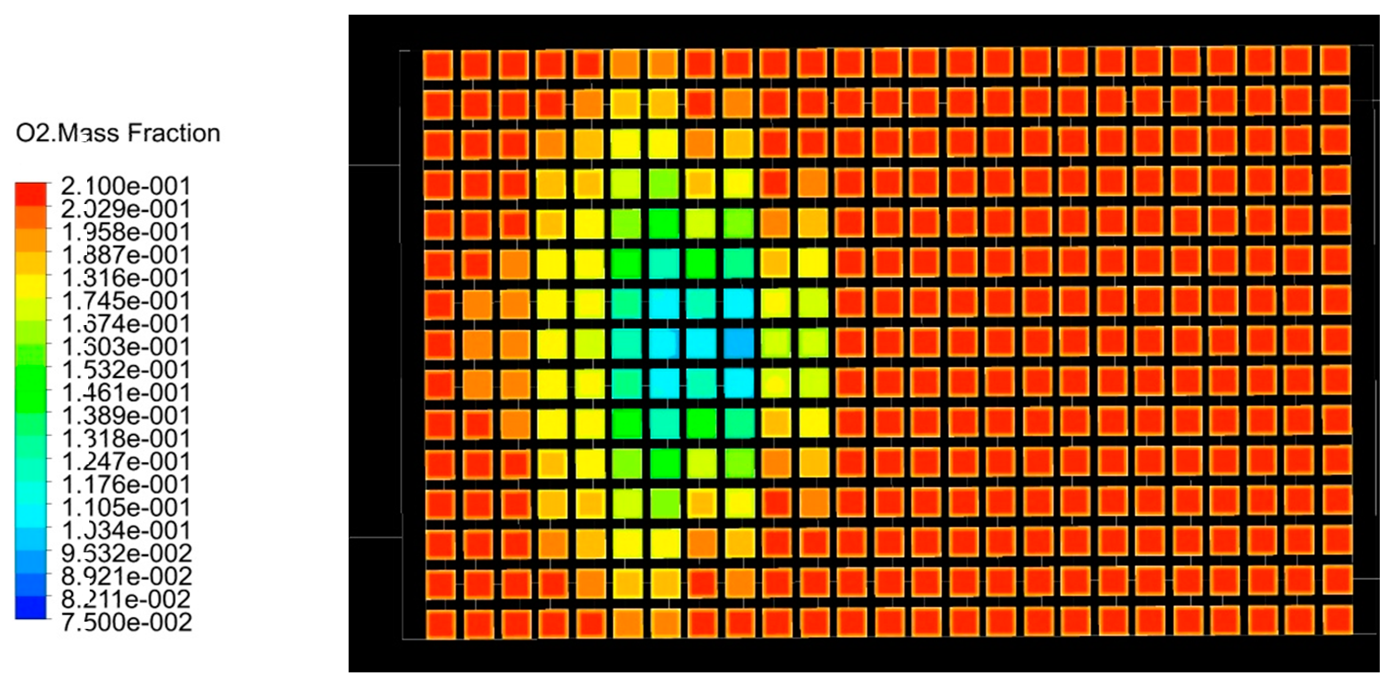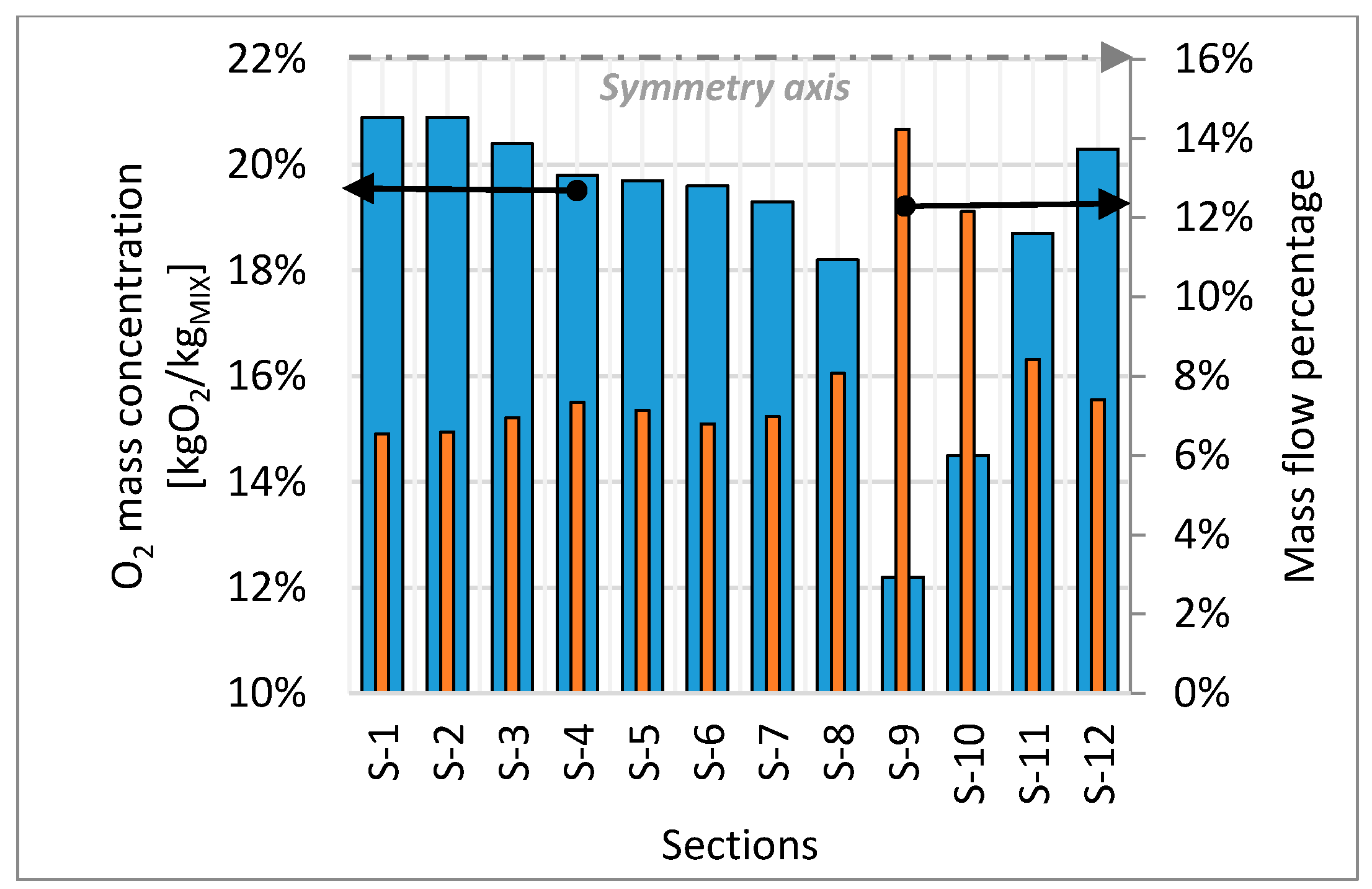Figure 10 shows the oxygen concentration pattern in the stacker cross section at the stacking top. In Figure 11, the previous control surface of Figure 10 is discretized into twelve rectangular sections where the O2 and the mass flow distributions are plotted. From these analyses, it is clear that the waste gas flow fills only the first part of the chamber. The above experience gained from the application of 3D CFD has been used to inspire the WGR effects modeling into the present lower order code. The Cold RC is cut across its symmetry axis into three geometrical identical sub-sections in order to simulate the thermal effects from the WGR system. At each subsection, the mass flow, the fluid temperature, and the chemicals mass fraction are specified as boundary conditions (see

Table 3. Parameters values of the Cold RC with the Waste Gas Recirculation (WGR) system.

	Tot	S-1	S-2	S-3
Volume [m3]	100	33.3	33.3	33.3
Heat transfer surface [m2]	2900	966.7	966.7	966.7
Mass flow [kg/s]	4.52	1.13	1.13	2.26
Waste gas mass fraction	20%	0%	10%	35%
Inlet temperature [C]	205	147	186.5	243.4

). The above values can be obtained from a reference CFD solution (as in the present example) or taken from a range based on the experience gained using CFD on similar configurations.

The profiles of the heat exchange coefficient for the Cold RC are obtained by adding to the reference linearized profiles [17] (valid for a standard regenerative system) the radiant effect introduced by the gas emission model presented in [20].

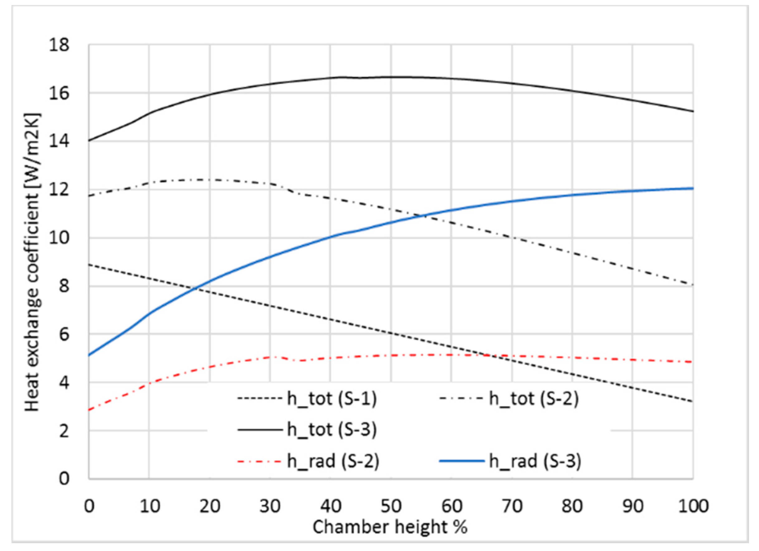
Figure 12 shows the heat transfer coefficient profile for each Cold RC sub-section. The first section is not fed with the waste gas (no radiant effect added), while the second and third sections have significant waste gas fraction; this explains the important heat transfer coefficient increase due to the radiant effect.

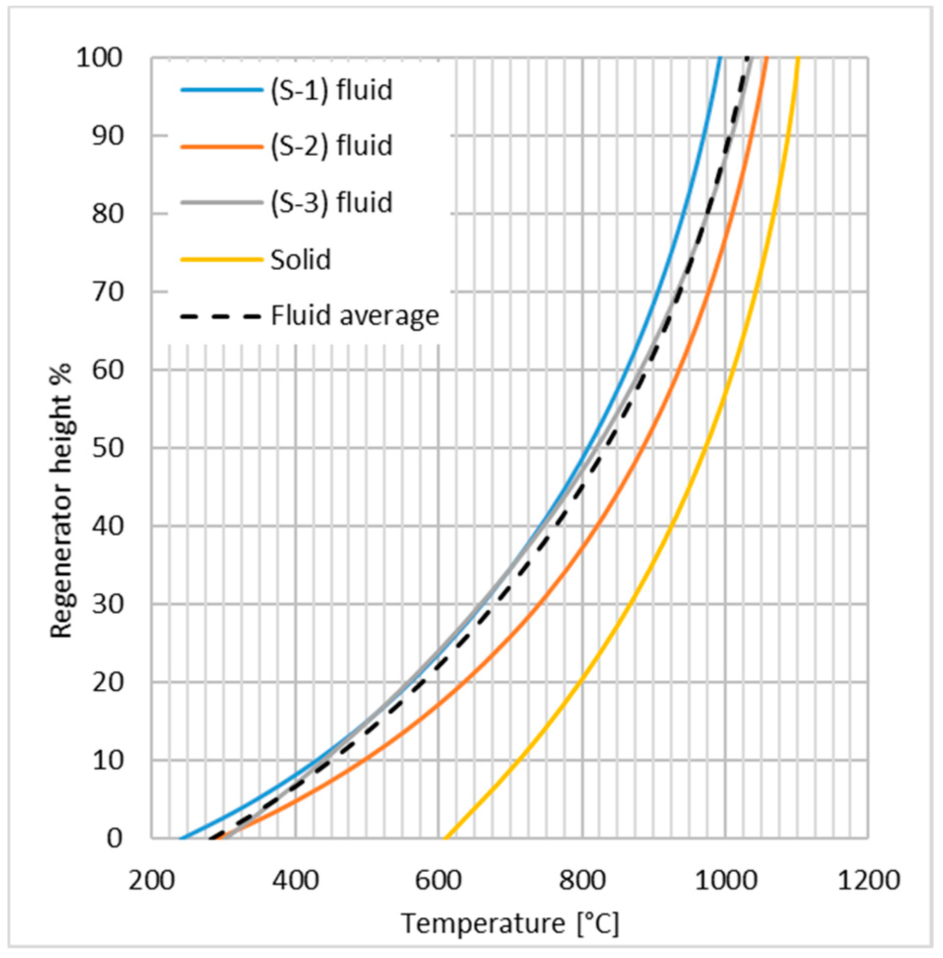
Figure 13 shows the mean temperature profile for each Cold RC sub-section. It can be seen that the fluid temperature profile is closer to the solid thermal profile in the S-2 and S-3 sections, i.e., where there is a waste gas fraction, than it is in the S-1 section.

In order to understand the WGR thermal effects on the exchanged thermal power $P_{th}$, each regenerator subsection is calculated using Equation (31).

$$P_{th}={\dot{m}}_f\left(c{p}_{f,in}{T}_{f,in}-c{p}_{f,out}{T}_{f,out}\right)$$

(31)

The specific thermal power (the thermal power referred to one square meter of heat transfer surface) is compared to the numerical results obtained without the WGR system (see

Table 4. Model output of the Cold RC with the WGR system.

	WGR off	WGR on - Average WG Fraction 20%
	-	Tot	S-1	S-2	S-3
Mass flow [kg/s]	4.52	4.52	1.13	1.13	2.26
WG mass fraction [%]	0	20	0	10	35
Inlet temperature [C]	150	205	147	186	243
Outlet temperature [C]	968	1018	983	1052	1019
Thermal power $P_{th}$ [MW]	3.09	3.74	0.945	0.991	1.81
Specific Thermal power [kW/m2]	1.065	1.290	0.978	1.025	1.872

).

It can be observed that, as far as the fluid exit temperature is concerned, the first section has a low temperature, about 983 °C, due to the low heat transfer. It is interesting to note that the second section gives the maximum outlet temperature of about 1052 °C, although it has a smaller heat transfer compared to the third one. This effect is due to the distribution of the mass flow rate and to the different inlet temperature of the flowing mixture.

The specific heat power increases from 0.97 kW/m² in the first regeneration section to 1.87 kW/m² in the third section. The average value in the case of the WGR with 20% of waste gas fraction is 1.29 kW/m² compared to 1.06 kW/m² with the system without the WGR. The total heat flux to the air with the WGR is about 3.75 MW with an increase of about 17% with respect to a standard regenerator.

The bulk temperature of the preheated air is 1018 °C with the WGR system; an increase of about 50 °C is obtained with respect to the standard regeneration system. The above effects confirm that the WGR system is effective not only for the NOx reduction process (as confirmed by the experimental tests [19]) but also for enhancing the thermal efficiency of the thermal regenerative process.

5. Conclusions

A one-dimensional transient model for the analysis of regeneration systems for glass furnaces is presented. This lower order model that allows a quick simulation of the regenerative set performance uses heat transfer coefficient profiles obtained from the application of specific CFD models. The heat transfer coefficients are locally re-computed in the code, taking into account the local composition of the gas according to the WGR strategy. A gas emissivity routine previously developed by the authors is used for the above heat transfer model. The model has shown its ability to simulate the effects of regenerator geometry or inversion time change. It can therefore be routinely used for the optimization of the refractory material distribution along the axis of the regenerative chambers during the system design. The model, extended to take into account the WGR effects, is applied to compare the regenerative system performance change with respect to the standard design. The analyses show an increase of the thermal performance of the regenerator when the WGR system is activated (air outlet temperature increase of about 50 °C in the example). The model proved to be a useful tool for understanding and quantifying the additional thermal effect introduced with the addition of radiant gases into the chamber when operating in the air phase according to the WGR strategy.