A New Method of GPS Water Vapor Tomography for Maximizing the Use of Signal Rays

Abstract

The spatio-temporal distribution of atmospheric water vapor information can be obtained by global positioning system (GPS) water vapor tomography. GPS signal rays pass through the tomographic area from different boundaries because the scope of the research region (latitude, longitude, and altitude) is designated in the process of tomographic modeling, the influence of the geographic distribution of receivers, and the geometric location of satellite constellations. Traditionally, only signal rays penetrating the entire tomographic area are considered in the computation of water vapor information, whereas those passing through the sides are neglected. Therefore, the accuracy of the tomographic result, especially at the bottom of the area, does not reach its full potential. To solve this problem, this paper proposes a new method that simultaneously considers the discretized tomographic voxels and the troposphere outside the research area as unknown parameters. This method can effectively improve the utilization of existing GPS observations and increase the number of voxels crossed by satellite signals, especially by increasing the proportion of voxels penetrated. A tomographic experiment is implemented using GPS data from the Hong Kong Satellite Positioning Reference Station Network. Compared to the traditional method, the proposed method increases the number of voxels crossed by signal rays and the utilization of the observed data by 15.14% and 19.68% on average, respectively. Numerical results, including comparisons of slant water vapor (SWV), precipitable water vapor (PWV), and water vapor density profile, show that the proposed method is better than traditional methods. In comparison to the water vapor density profile, the root-mean-square error (RMS), mean absolute error (MAE), standard deviation (SD), and bias of the proposed method are 1.39, 1.07, 1.30, and −0.21 gm⁻³, respectively. For the SWV and PWV comparison, the RMS/MAE of the proposed method are 10.46/8.17 mm and 4.00/3.39 mm, respectively.

1. Introduction

Although atmospheric water vapor comprises only a small percentage of the atmosphere, it plays a key role in a series of weather phenomena [1,2]. A good understanding of the spatiotemporal changes in water vapor is helpful in improving weather prediction, water resource management, and natural hazard reduction [3,4,5,6,7,8,9]. Compared with traditional water vapor acquisition methods, such as a radiosonde and microwave radiometer, global positioning system (GPS) tomography has the advantage of a high temporal and spatial resolution, and low construction and maintenance costs [10,11,12,13,14].

The concept of water vapor tomography, which refers to the usage of GPS signals as scanning rays in the tomographic grid, was first proposed by Braun et al. and realized by Flores et al. [15,16]. In GPS water vapor tomography, the research area is covered by ground GPS receivers and discretized into several voxels [17]. The integral equations established by the signal observations are utilized to calculate the wet refractivity or water vapor density within each voxel [18].

Signal rays penetrate not only from the top boundary of the area, but also from the side face due to the specific distribution of the satellite constellation and receivers and the specific choice of the tomographic area. Traditional methods, which use only the first-mentioned signal rays above, reduce the utilization of GPS observation data and the accuracy of the tomographic result, especially at the bottom of the area. To solve this problem, Rohm and Bosy estimated the outer part of the signal rays using the UNB3m model based on a ray-tracing method [17], Notarpietro et al. used European center for medium-range weather forecasts (ECMWF) data to calculate the SWV outside the research area [19], and Chen and Liu applied the numerical weather prediction (NWP) profile data to estimate the slant wet delay (SWD) outside the modeling area [20]. Benevides et al. proposed a geometric linear method using an empirically exponential negative function to increase the utilization of signal rays [21], whereas Yao et al. introduced a unit scale factor model and reconstructed a sophisticated model for considering the signal rays penetrating from the side face of the study area [22,23].

In the above-mentioned methods, their focus is to calculate SWV values of the signal ray generated outside the tomographic grid, which needs external data or models, such as ECMWF, NWP, and UNB3m. This work proposes a new method that does not feature external data and considers and models the troposphere outside the research area as unknown parameters for tomographic modeling to improve the utilization of existing GPS observations and increase the number of voxels crossed by satellite signals. Additionally, contrast methods were conducted to verify the performance of the proposed method.

2. Methods

2.1. GPS Water Vapor Estimation

In this study, the SWV derived from GPS-based receivers is exploited to obtain the water vapor distribution information. The SWV can be obtained by the following formula [24,25]:

$$\mathrm{SWV}=\frac{{10}^6}{{\rho }_{water}{R}_{\omega }\left[\left(k_3/T_m\right)+k_2^{\prime }\right]}\times \mathrm{SWD}$$

(1)

where ${\rho }_{water}$ is the density of liquid water; $R_{\omega }=461J/\left(kg\cdot K\right)$ is the specific gas constants for water vapor; $k_2^{\prime }=16.48KhP{a}^{-1}$ and $k_3=3.776\times {10}^5{K}^{2}hP{a}^{-1}$ are constants; and $T_m$ is the weighted mean tropospheric temperature, which is calculated by an empirical formula [26]. In order to obtain the SWD, the ZWD and the wet delay gradient parameters should be mapped into the elevation direction and the unmodeled residuals should be taken into account [27,28]. The specific calculation formula is as follows:

$$\mathrm{SWD}=m_w\left(e\right)\ast \left[\mathrm{ZWD}+\cot \left(e\right)\left(G_{NS}^w\ast \cos \phi +G_{WE}^w\ast \sin \phi \right)\right]+R$$

(2)

where $e$ and $\phi$ are the satellite elevation and azimuth, respectively; $m_w$ is the wet mapping function; $R$ denotes the unmolded residuals; $G_{NS}^w$ and $G_{WE}^w$ are wet delay gradient parameters in the north–south and east–west directions, respectively; and ZWD is the zenith wet delay, which can be calculated by subtracting the zenith hydrostatic delay from the zenith total delay.

2.2. Traditional Tomographic Equation

In water vapor tomography, the tomographic equation consists of two types of equations, one is the observation equation and the other is the constraint equation. The observation equation is the core of water vapor tomography, which is based on the water vapor integral along the signal ray path. The constraint equation contains horizontal and vertical constraints.

2.2.1. Observation Equation

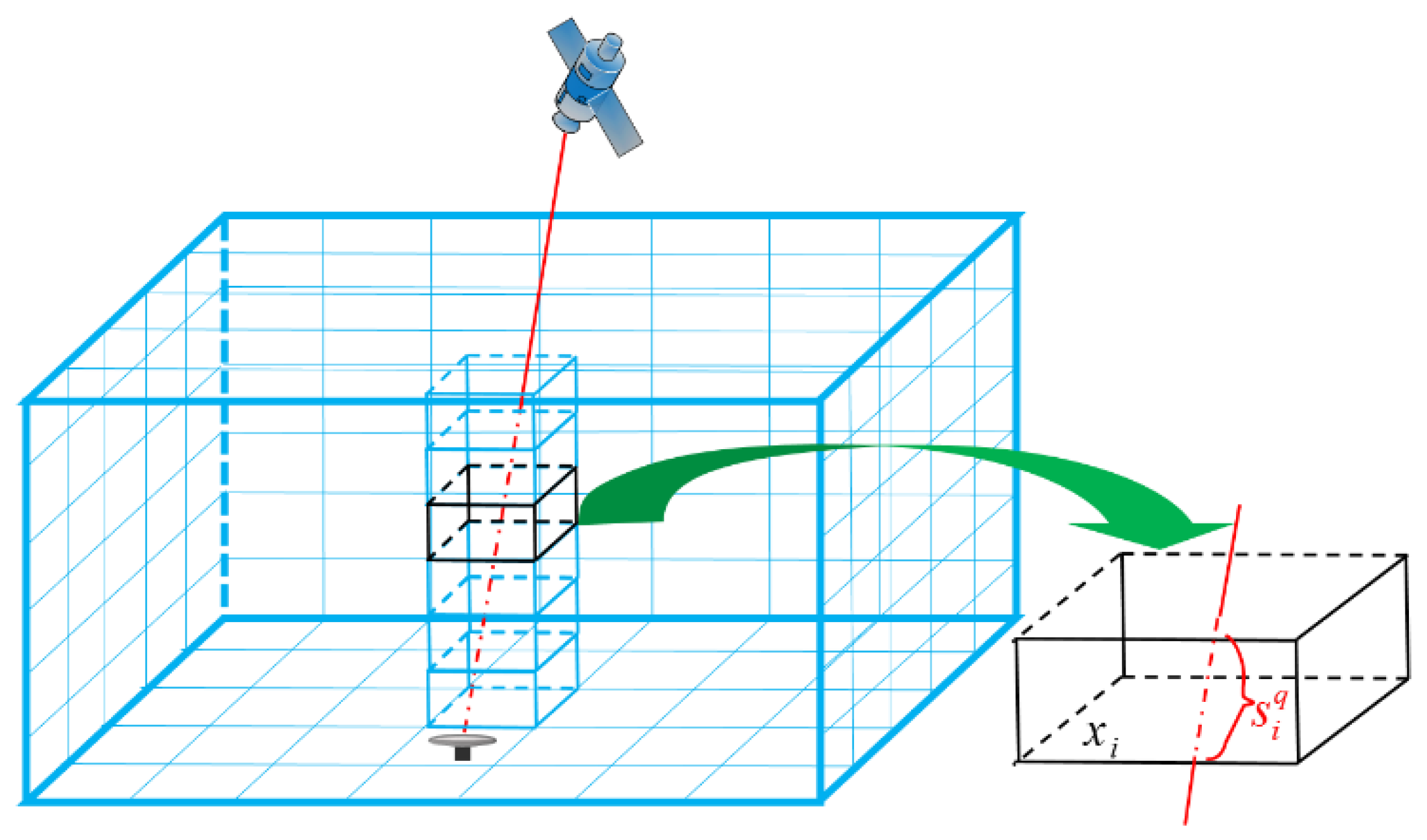
The whole research area and the water vapor density in the discretized tomographic voxel are shown in Figure 1, and the observation equation can be established on the basis of the GPS signal crossing as follows:

$${\mathrm{SWV}}^q={\displaystyle \sum _{i=1}^n{s}_i^q\cdot x_i}$$

(3)

where superscript $q$ denotes the satellite index; $n$ is the total number of discretized tomographic voxels; $s_i^q$ represents the length of the satellite signals within the voxel, which can be calculated by the coordinates of two intersections; and $x_i$ is the water vapor density of the voxel, i.

2.2.2. Constraint Equations

The tomographic result only utilizing the observation equation is typically undetermined in the inversion process. The source of this undetermined nature is related to SWV paths not penetrating every voxel and that the SWV observations have similar geometry (i.e., from a GPS satellite to a station). To overcome this inversion problem, the mostly widely-used method is to impose constraint information [29].

In the research area, the water vapor density, $x_i$, within a certain voxel can be represented by the weighted average of its neighbors because of the relatively stable horizontal distribution [30,31]. The specific horizontal constraint equation is as follows:

$$w_1^i{x}_1+w_2^i{x}_2+\cdots w_{i-1}^i{x}_{i-1}-x_i+w_{i+1}^i{x}_{i+1}+\cdots +w_m^i{x}_m=0$$

(4)

where $m$ is the total number of voxels in the same layer and $w$ denotes the horizontal weighting coefficient, which can be computed by the Gaussian weighting function as follows:

$$w_{i-1}^i=d_{i,i-1}/{\displaystyle \sum _{j=1}^m{d}_{i,j}}$$

(5)

where $d$ is the distance between the centers of the two corresponding voxels.

The vertical constraint equation is established using the empirical formula of the water vapor density between two adjacent layers:

$$x_j-p_{j+m}\cdot x_{j+m}=0$$

(6)

where $x_j$ and $x_{j+m}$ denote the water vapor density in the voxel, $j$ and $j+m$, respectively, and $p_{j+m}$ is the vertical weighting coefficient, which can be obtained as follows:

$$p_{j+m}=e^{\left(h_{j+m}-h_j\right)/H}$$

(7)

where $e$ is the Euler’s number and is approximately equal to 2.718, and H is the water vapor scale height, which is set as 1–2 km.

2.3. New Tomographic Equation

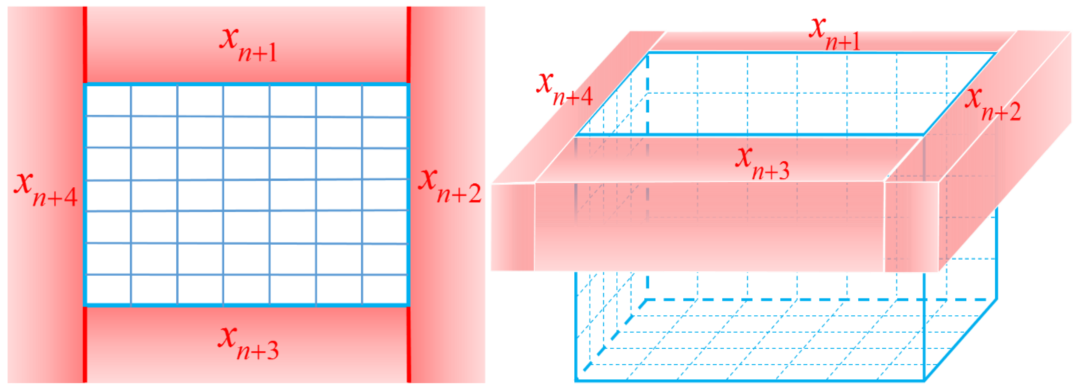
As shown in Figure 1, the research area is divided into n voxels and the water vapor density of each voxel is $x_i\left(i=1,2\cdots n\right)$ in the traditional method. To improve the utilization of GPS data, the water vapor density in the four directions outside the research region are added to the observation equation as unknown parameters. Figure 2 displays the four new parameters ($x_{n+1}$, $x_{n+2}$, $x_{n+3}$, and $x_{n+4}$ for the north, east, south, and west, respectively) in the proposed method from a top view (left) and a side view (right). The boundaries of these four regions are selected based on the location of GPS receivers and the specifics of the tomographic area (see the process in the following experiment). The observation equation of the proposed method is as follows:

$${\mathrm{SWV}}^q={\displaystyle \sum _{i=1}^n{s}_i^q\cdot x_i}+\left(s_{n+1}^q\cdot x_{n+1}+s_{n+2}^q\cdot x_{n+2}+s_{n+3}^q\cdot x_{n+3}+s_{n+4}^q\cdot x_{n+4}\right)$$

(8)

This equation is similar to that in the traditional method; only the four parameters in the parentheses are added. The distances produced by satellite rays outside the research area are expressed as $s_{n+1}^q,s_{n+2}^q,s_{n+3}^q,s_{n+4}^q$ and they equal 0 when the signal rays penetrate from the top boundary of the area. The new functional model for the water vapor tomography comprises the new observation equation and the constraint equation, which is described as:

$$\left(\begin{array}{c}{\mathrm{SWV}}_{q\times 1}\\ 0_{n\times 1}\\ 0_{(n-m)\times 1}\end{array}\right)=\left[\begin{array}{c}{A}_{q\times (n+4)}\\ H_{n\times (n+4)}\\ V_{(n-m)\times (n+4)}\end{array}\right]\cdot X_{(n+4)\times 1}+\left[\begin{array}{c}\Delta 1_{q\times 1}\\ \Delta 2_{n\times 1}\\ \Delta 3_{(n-m)\times 1}\end{array}\right]$$

(9)

where A from Equation (8), H from Equation (4), and V from Equation (6) represent the coefficient matrices of the new observation equation, the horizontal constraint equation, and vertical constraint equation, respectively; $X=\left[x_1,x_2,\cdots ,x_n,\cdots ,x_{n+4}\right]$ is a vector of the water vapor density containing all voxels to be estimated; ${\Delta }_1,{\Delta }_2,{\Delta }_3$ are the noises of the new observation equation, the horizontal constraint equation, and vertical constraint equation, respectively.

3. Experiment Description

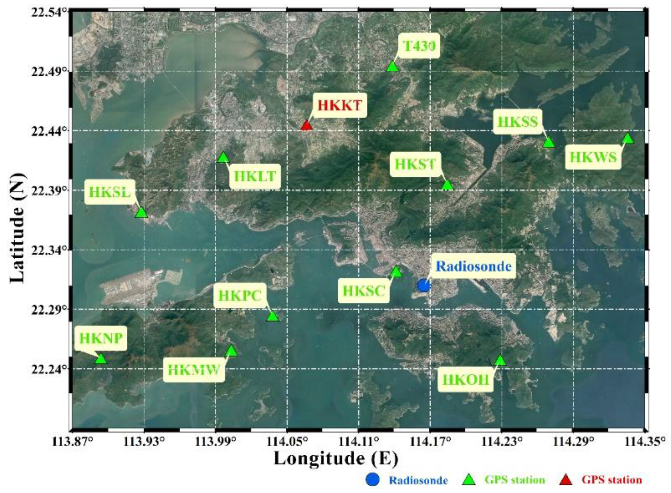
The tomographic experiment is implemented using data from 12 stations (HKLT, HKMW, HKNP, HKOH, HKPC, HKSC, HKSL, HKSL, HKSS, HKST, HKWS, T430 for tomographic modeling and HKKT for SWV comparison) of the Hong Kong Satellite Positioning Reference Station Network (SatRet) for a week (June 1–7, 2017). Figure 3 shows the GPS station distribution, the division of the grids, and radiosonde station 45004. GAMIT (v.10.61) is used to process the GPS data with a sampling interval of 30 s. The wet mapping function and the empirical formula of the weighted mean tropospheric temperature are used to project SWV on the basis of Equations (1) and (2). The tomographic period is 30 min and 48 tomographic experimental solutions can be processed every day.

The scope of the tomographic region is (113.87°, 114.35°) for longitude, (22.19°, 22.54°) for latitude, and (0, 8 km) for altitude. The horizontal resolutions in the east–west and north–south directions are 0.06° and 0.05°, respectively, and the vertical resolution is 800 m. It should be noted that water vapor density of the outer region (the north, east, south, and west) can be expressed by an unknown parameter ($x_{n+1}$, $x_{n+2}$, $x_{n+3}$, and $x_{n+4}$), provided that the water vapor density in that region changes are relatively stable and as many as possible signal rays from the side face can be included in the region. To find the boundaries of the outer region that meet the above two requirements, the law of water vapor change, the size of the research area, and the distribution of the stations need to be carefully studied. The specific steps are as follows:

• To analyze the law of water vapor change. Figure 4 shows the relationship between water vapor density and altitude during the study period, with the red line being the fitted curve (upper for 45005, middle for 59,280, and lower for 59,316, respectively). The stations, 59,280 and 59,316, are located outside the tomographic area and their coordinates are (23.66°, 113.05°) and (23.35°, 116.66°), respectively. We can see that the water vapor concentrates in the lower troposphere, where it also changes more rapidly than above. In order to obtain the function between water vapor density (x) and altitude (h), the polynomial fitting method was used. Equation (10) was estimated by taking the altitude as the independent variable, while the water vapor density was regarded as the independent variable in Equation (11):

  $$x=26.34-9.22\ast {10}^{-3}h+1.19\ast {10}^{-6}{h}^2-5.51\ast {10}^{-11}{h}^3$$

  (10)

  $$h=7704.64-923.77x+47.90x^2-0.93x^3$$

  (11)
• To find the suitable altitudinal boundary of the outer region. It can be computed by Equation (10) that the value of the water vapor density near the surface is 26.34 g/m³. The range of the water vapor density in this research area is considered as around 0–26.34 g/m³. For 10 layers in the altitude direction, if the change of the water vapor density with altitude in the outer region is within 0 to 2.634 g/m³, it can be defined as a stable outer region. From Equation (11), the water vapor density of 2.634 g/m³ corresponds to the height of 5586 m. Considering the convenience of rectification and the error caused by fitting, 5500 m can be selected as the alternative to the suitable altitudinal boundary of the outer region.
• To decide the boundaries of the outer region in the east–west and north–south directions. The signal rays of all experimental periods acquired by satellite receivers in the research area are collected and their paths in the tomographic grid are calculated. Then, the signal rays passing through from the side face are extracted and divided to two parts, one of which are signals penetrating from the side face at a height greater than 5500 m. Additionally, the intersections of this part of the signal rays with the top layer, namely the layer of 8 km, are counted. The boundaries of the outer region in the east–west and north–south directions are decided by the distribution of these intersections.
• To check the boundaries of the outer region. If the horizontal range of the outer region is within twice the length of a voxel, the reasonable boundaries of the outer regions are achieved. Otherwise, go back to Step 2, increase the value of the altitudinal boundary, and re-proceed to the next steps.

After these procedures, the boundaries of the outer regions are determined in the Hong Kong experiment, the boundary for altitude is 5.5 to 8 km, and the boundaries of the four directions (the north, east, south, and west) are 22.59°, 114.43°, 22.11°, and 113.84°, respectively. Therefore, a total of 8 × 7 × 10 voxels in the research area and four extra unknown parameters outside the research area are obtained.

To evaluate the performance of the proposed method, we made tomographic solutions using the traditional method with 8 × 7 × 10 voxels, identified as Scheme #1, and the new method above-mentioned, identified as Scheme #2. In addition, Scheme #3 is to extend the size of the entire tomographic area, that is, the scope is changed to (113.81°, 114.41°) for longitude, (22.14°, 22.59°) for latitude. The new scope, which results in 10 × 9 × 10 voxels in the tomographic modeling, is nearly to the outer boundaries of Scheme #2. For Scheme #3, the horizontal resolution in the east-west and north-south direction are 0.06 and 0.05, respectively, and the vertical resolution is 800 m, which is the same as that in Scheme #1. Since the outer regions in Scheme #2 are included, Scheme #3 can also utilize the increased signal rays of Scheme #2 in the tomographic solutions.

4. Results and Discussion

4.1. Utilization of Voxels and Signal Rays

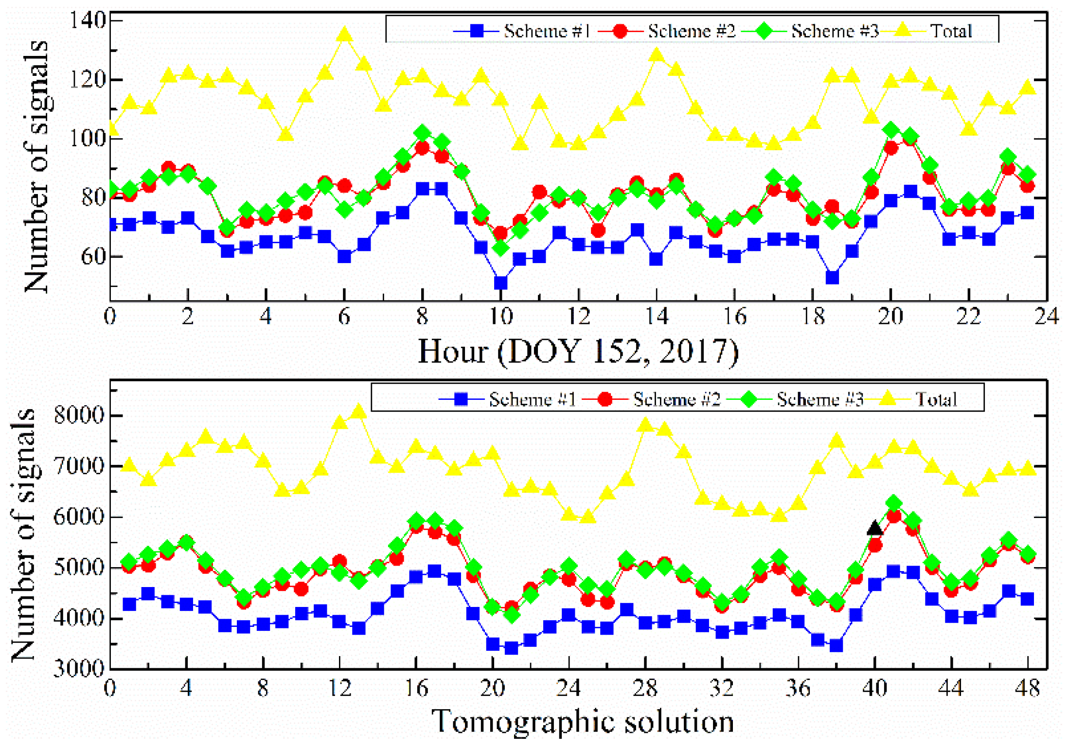
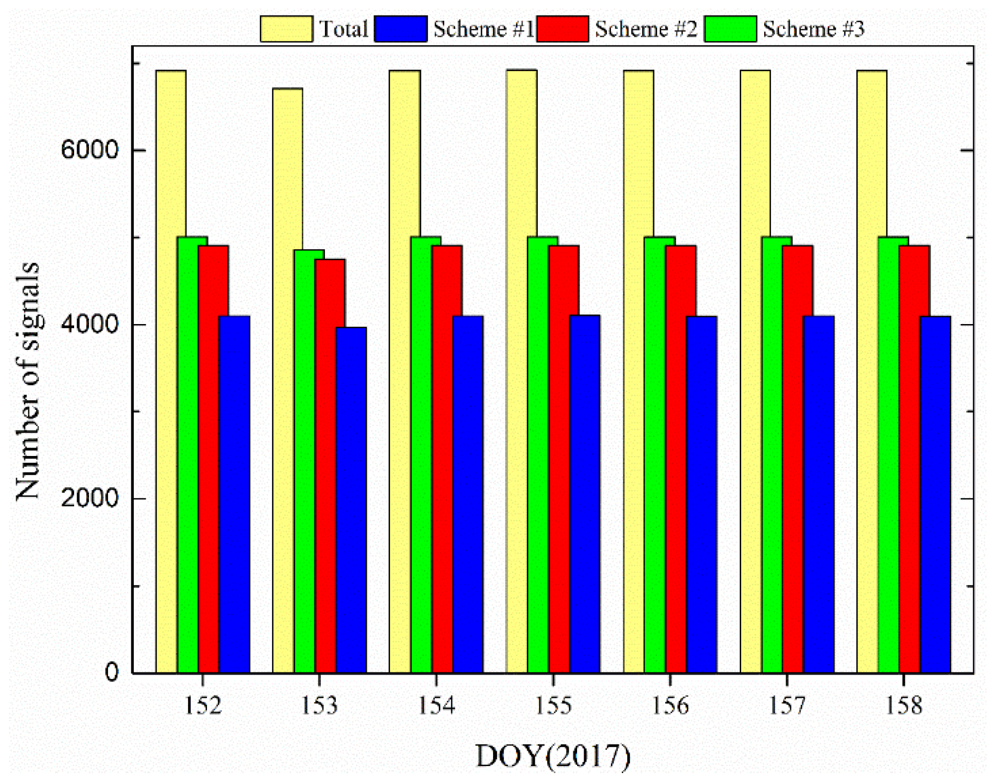
To compare the influences of different methods on the number of signal rays used, the experimental results were analyzed. Figure 5 shows the number of signal rays used in different schemes at day of year (DOY) 152, 2017, the upper one for the case of per 30 min, and the lower one for each tomographic solution. It can be seen that only a small part of the signal rays is used in Scheme #1 compared with the total number of signal rays observed. Scheme #2 improves the utilization of signal rays in every epoch and solution, and Scheme #3 has the same effect in improving the usage of signal rays, which illustrates that Scheme #3 can be a good comparison to Scheme #2. Moreover, the average number of signal rays observed, used in different schemes, can be seen in Figure 6. The figure illustrates that Scheme #2 improves the average utilization of signal rays used by 19.68% compared with Scheme #1. For Scheme #3, the percentage of increment is 22.2%.

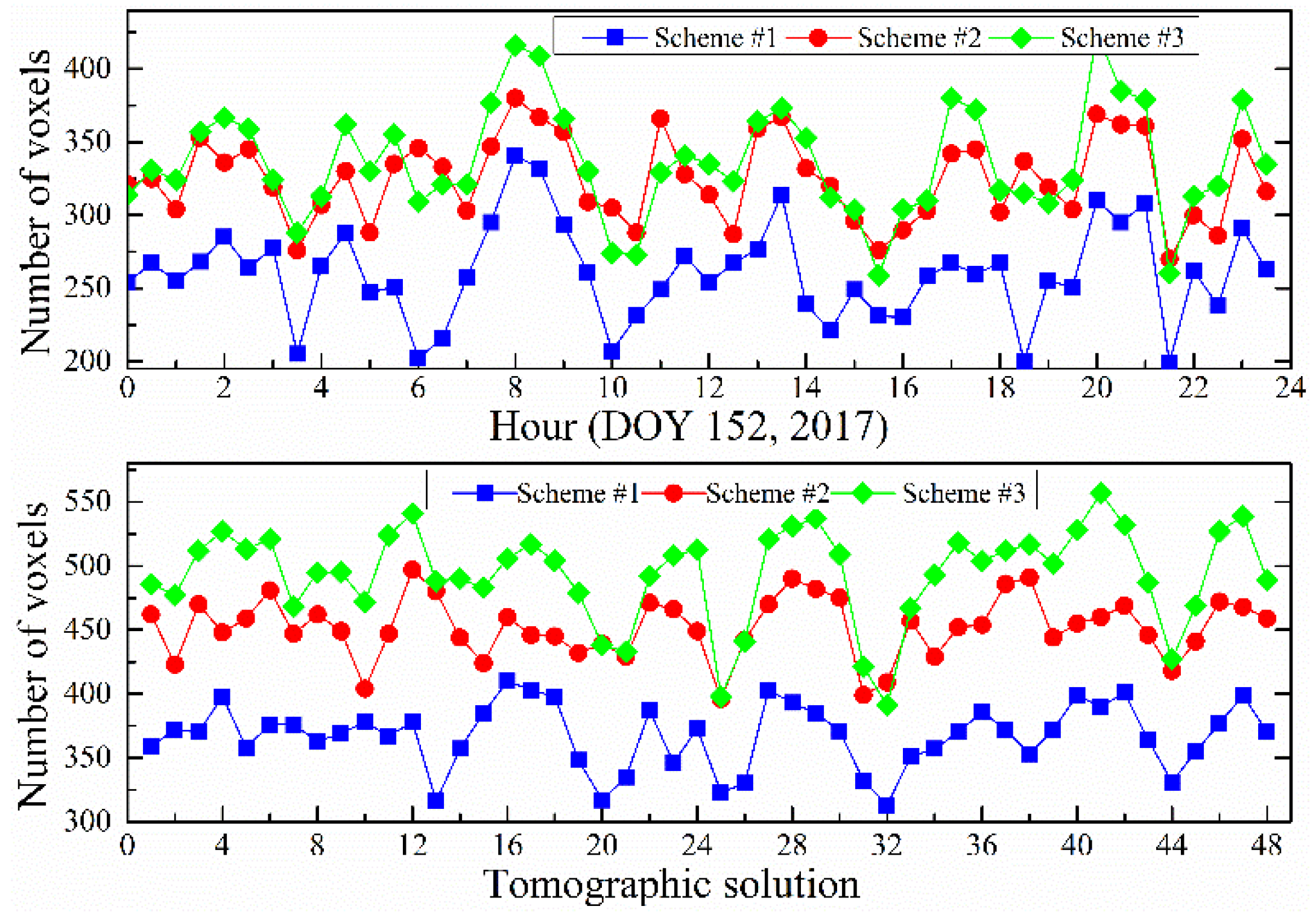
On the other hand, the number of voxels passing through by the signals is analyzed. The upper image in Figure 7 shows the number of voxels crossed by the signal rays once per 30 min between Schemes #1, #2, and #3, whereas the lower image shows the situation of every tomographic solution in that day. Evidently, the number of voxels crossed by the signal rays in Scheme #2 is more than that of Scheme #1, both for an epoch or a tomographic solution. For Scheme #3, it has the largest number of voxels crossed by signal rays in most cases, but it does not represent a good performance in penetrating voxels for Scheme #3. This is because the total number of voxels in Scheme #3 is 900, which is much larger than 560 in the other schemes. It may make more sense to focus on the percentage of the voxels crossed by signal rays.

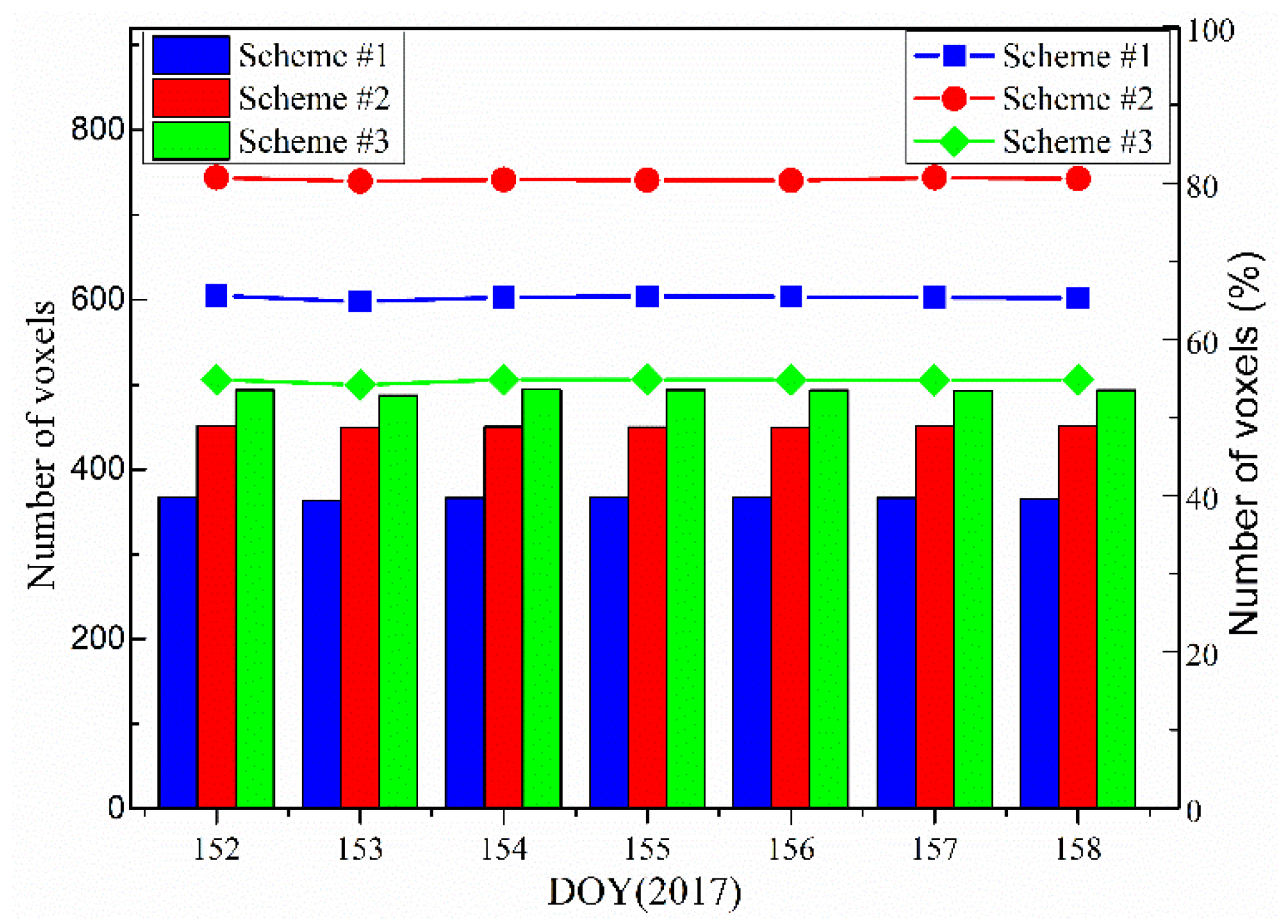
Moreover, the statistical results, which include the average number and percentage of voxels crossed by signal rays once per day in different schemes for the period of DOY 152–158, 2017, can be seen in Figure 8. The finding shows that the average number of Scheme #1 increases by 15.14% from 65.36% to 80.50% under Scheme #2. Additionally, Scheme #3 has the largest value in the average number of voxels, but its percentage (54.74%) of voxels crossed by signal rays is the smallest. For models with different total voxels, the percentage of voxels passing though by signal rays is more important than the number of that.

4.2. PWV Comparison

To assess the accuracy of the tomographic result, the PWV value for the location of the radiosonde station is calculated using the water vapor density of the voxels acquired from the three schemes and compared with PWV derived from the radiosonde data at UTC 0:00 and 12:00. In this experiment, eight tomographic solutions are selected daily to calculate PWV. As shown in Figure 9, the trends of the PWV time series are basically consistent and the results of Scheme #3 agree worst with that from the radiosonde. Compared with Scheme #1, it is clear that Scheme #2 is more consistent with the radiosonde data, indicating that the proposed method can improve the tomographic accuracy. The statistical results are listed in

Table 1. Statistical results of PWV between various schemes and radiosonde for the week of DOY 152–158, 2017 (unit: mm).

	RMS	MAE	Bias
Scheme #1	5.06	4.40	4.11
Scheme #2	4.00	3.39	2.76
Scheme #3	5.72	5.21	4.23

, which show an advantage of Scheme #2 compared with other schemes in terms of RMS, MAE, and bias.

4.3. Water Vapor Profile Comparison

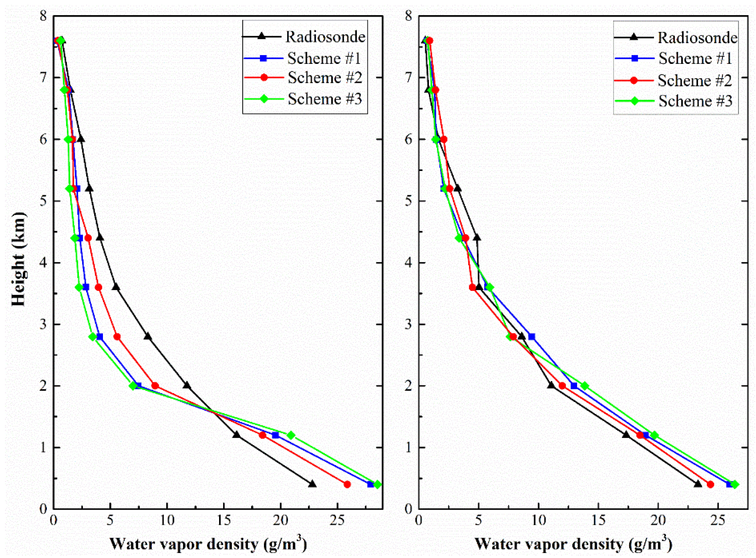
In general, if two vertical layers are exchanged arbitrarily, then the PWV remains the same, but the vertical distribution of the water vapor changes. Therefore, the PWV comparison mentioned above may not denote a correct tomographic result obtained, although the PWV derived from the different schemes are in good agreement with that from the radiosonde. To validate the accuracy of the vertical water vapor density, the water vapor profiles between the radiosonde and the two schemes are compared, as shown in Figure 10. Two dates are selected because they correspond to the maximum and minimum RMS during the week-long experimental period.

Figure 10 shows that the tomographic water vapor profiles of the three schemes agree well with those from the radiosonde data. The water vapor density profile of Scheme #2 better matches that from radiosonde than the other two schemes, especially in the low layers. Scheme #3 has the worst performance. Compared with radiosonde, the numerical results of the tomography from Scheme #2 for the two selected epochs (RMS are 1.90 and 0.78 g/m³) are superior to those of Scheme #1 (RMS are 2.98 and 1.32 g/m³) and Scheme #3 (RMS are 3.37 and 1.67 g/m³).

Table 2. Statistical results of water vapor profile comparisons between radiosonde and different schemes for the period of DOY 152 to 158, 2017 (unit: g/m³).

		Scheme #1	Scheme #2	Scheme #3
RMS	Mean	1.97	1.39	2.23
	Max	2.98	1.90	3.37
	Min	1.32	0.78	1.67
MAE	Mean	1.51	1.07	1.68
	Max	2.42	1.62	2.80
	Min	1.06	0.66	1.33
Bias	Mean	−0.33	−0.21	−0.41
	Max	0.59	0.53	0.72
	Min	−1.15	−0.87	−1.28
SD	Mean	1.87	1.30	2.11
	Max	2.89	1.82	3.30
	Min	1.17	0.76	1.56

lists the statistical results of the three schemes in all water vapor profile comparisons, including RMS, MAE, bias, and SD. The numerical results reveal that the average RMS/MAE/bias/SD values are 1.97/1.51/−0.33/1.87, 1.39/1.07/−0.21/1.30, and 2.23/1.68/–0.41/2.11 gm−3 for Schemes #1, #2, and #3, respectively. The maximum and minimum values of each statistic are shown in the table. These findings show that the proposed method is more consistent with the radiosonde data than the other two traditional methods. It should be noted that Scheme #3 does worse than Scheme #1, which indicates the total number of voxels and the selection of the entire tomographic area size are important to the tomographic result.

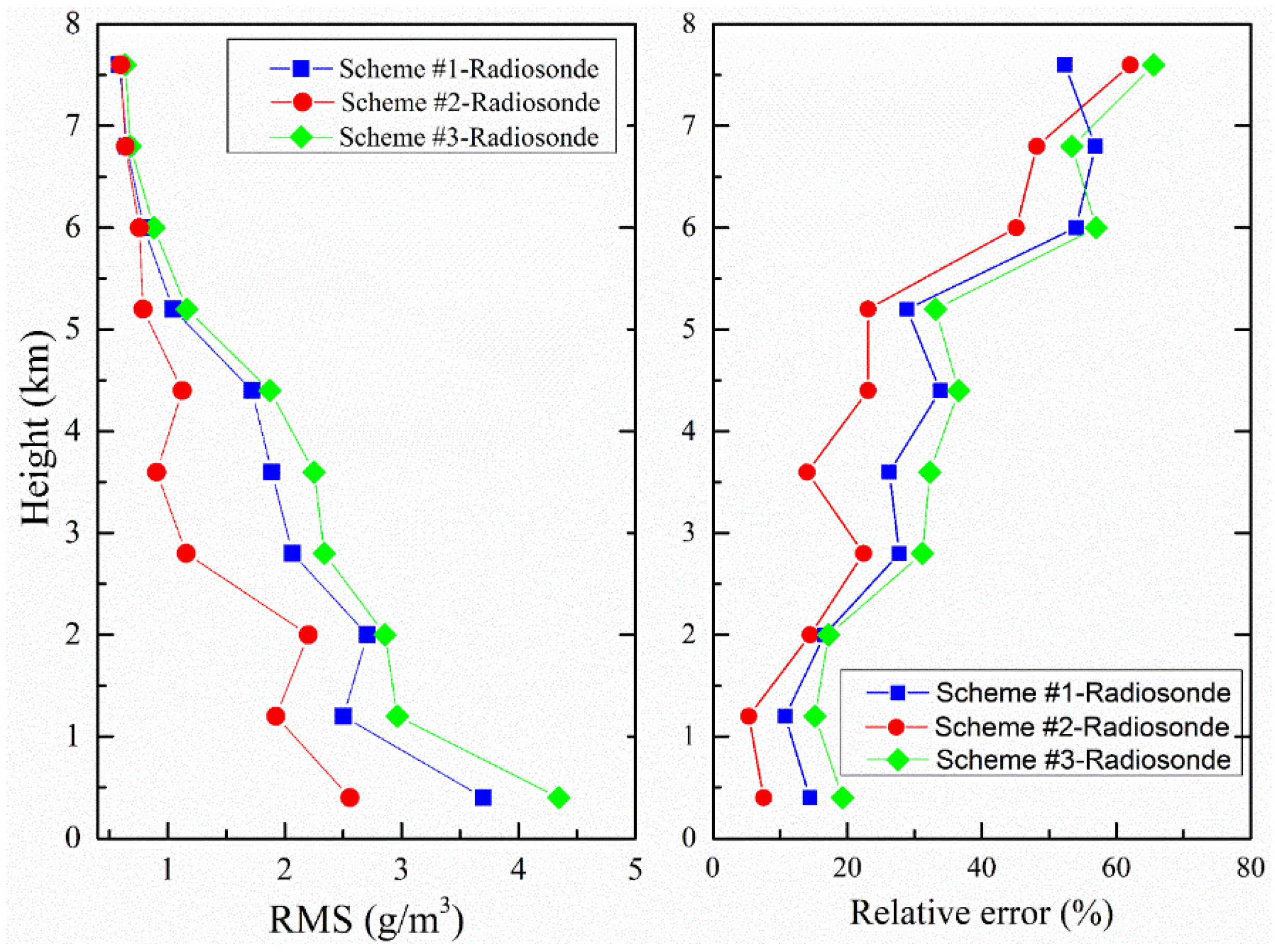
To make a further comparison of the relationship between the altitude and the errors in different schemes, the tomographic results (DOY 152–158, 2017) are analyzed. The average RMS error and relative error at different layers for the three schemes are calculated in this period to show the pattern of the vertical water vapor distribution and altitude. Figure 11 gives the RMS and relative error changes with height throughout the experimental period. It can be seen that the RMS, generally, decreases with altitude, whereas the relative error shows an opposite trend. A large relative error appears in the upper layers because the water vapor density is very low in those layers and a small discrepancy between the tomographic result and radiosonde data will result in a large value. In addition, the RMS and relative error of the proposed method (Scheme #2) are generally less than those of the traditional methods (Scheme #1 and #3) for the different layers, which validates the improved nature of the proposed method over the traditional methods.

4.4. SWV Comparison

To further evaluate the performance of the proposed method, the SWV of station HKKT is computed using the three schemes and their differences against the GAMIT-estimated SWV are identified. It should be noted that only the SWV penetrated from the top boundary in Scheme #1 were used in this comparison. To better show the results, SWV residuals are grouped into individual elevation bins of 5°, such that all residuals with an elevation angle between 15° and 20° are evaluated as a single unit. The RMS of each elevation bin are calculated and are shown in Figure 12, in which the upper and lower one represent the rainy and rainless scenario, respectively. It is clearly visible that the RMS of SWV residuals reduced as the elevation angle decreased. Colors in the figure indicate that better RMS results can be achieved by Scheme #2 in different weather conditions. Scheme #3 also is worse than Scheme #1 in this comparison. In summary, the residuals of SWV are reduced by the proposed method compared with the other two schemes.

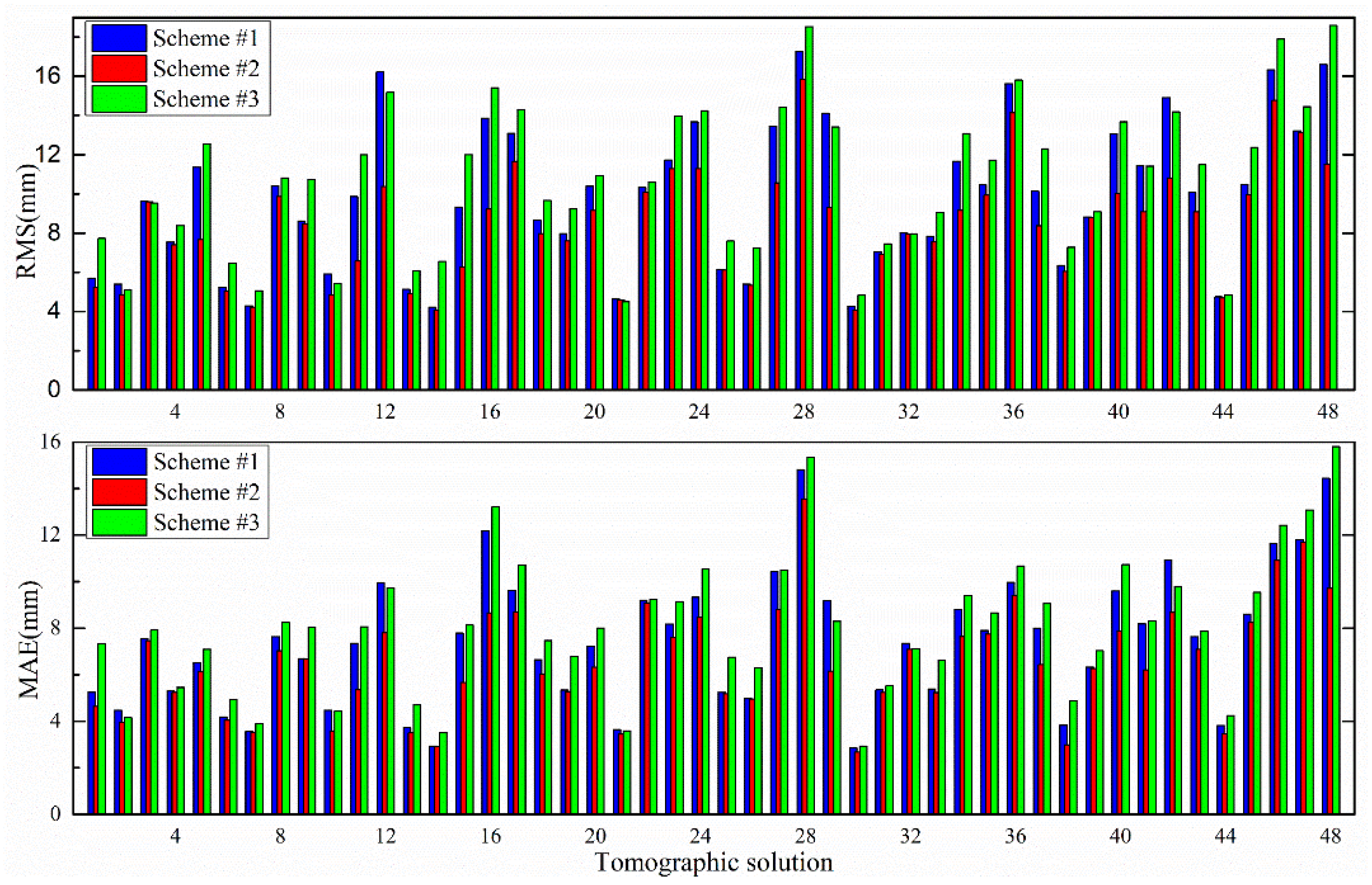
To further show the superiority of the proposed method in the SWV comparison, the RMS and MAE of every tomographic solution in DOY 152, 2017 are compared in Figure 13. The red marks acquired by Scheme #2 are smaller than the blue markers obtained by Scheme #1, and also smaller than the green markers obtained by Scheme #3 in the solutions of every period of time, which illustrates the superiority of the proposed method over the traditional methods. Moreover,

Table 3. RMS and MAE of SWV using Schemes #1 and #2 for 7 days (unit: mm).

DOY	RMS			MAE
	Scheme #1	Scheme #2	Scheme #3	Scheme #1	Scheme #2	Scheme #3
152	9.81	8.61	10.73	7.41	6.96	7.99
153	11.58	9.49	12.40	9.00	7.59	9.93
154	11.48	10.48	12.64	8.99	7.33	10.38
155	13.26	12.57	14.21	10.93	10.01	11.08
156	11.76	10.98	12.08	8.99	8.00	9.64
157	11.21	9.95	11.67	8.72	8.01	9.28
158	13.07	11.13	13.81	9.98	9.34	10.80
Average	11.74	10.46	12.51	9.15	8.17	9.87

shows the average RMS and MAE calculated from the three schemes for 7 days. A similar situation as that in Figure 13 shows that the RMS and MAE of SWV reduced by the proposed method in the experimental period from 11.74/9.15 mm (Scheme #1) and 12.51/9.87 mm (Scheme #3) to 10.46/8.17 mm, respectively. In summary, it is clear evidence that the proposed method improves the accuracy of the tomographic result.

5. Conclusions

The observation equations of GPS water vapor tomography are constructed by signal rays, and an increase in the quantity of signal rays added to the tomographic model contributes to an improved tomographic result. This paper proposed a new method that utilizes the signal rays coming from the top boundary and the side face of the tomographic area. Four outer regions were added to the tomographic equation as unknown parameters, and their boundaries were reasonably determined in the experiment. The traditional method using 8 × 7 × 10 voxels with the selected research area (Scheme #1) and another method using 10 × 9 × 10 voxels with an extended research area (Scheme #3) were utilized as comparisons.

The tropospheric parameters were estimated using GAMIT software based on the Hong Kong Satellite Positioning Reference Station Network. The tomographic experiment was subsequently conducted using the three schemes. Numerical results from DOY 152 –158, 2017 show that the proposed method increases the number of voxels crossed by signal rays (15.14% on average) and improves the utilization of the observed data (19.68% on average) in comparison with the traditional method (Scheme #1). For Scheme #3, the cost of increasing the number of signal rays and the quantity of voxels crossed by rays was to add voxels in total from 560 to 900, which makes the proportion of crossed voxels drop.

Radiosonde data were used as a reference to validate the tomographic result. In a comparison of the PWV time series, the RMS, MAE, and bias values of the proposed method were 4.00, 3.39, and 2.76 mm, respectively, which were smaller than those of the two traditional methods. A comparison of the water vapor density profiles at different altitudes showed that the profile of the proposed method matches the radiosonde data well. This finding was supported by the statistical results for RMS/MAE/bias/SD, which changed from 1.97/1.51/−0.33/1.87 gm⁻³ of Scheme #1 and 2.23/1.68/-0.41/2.11 gm⁻³ of Scheme #3 to 1.39/1.07/−0.21/1.30 gm⁻³ of Scheme #2. In addition, an SWV comparison using data from station HKKT was conducted using different schemes; the RMS and MAE values of the SWV changed from 11.74/9.15 mm of Scheme #1 to 10.46/8.17 mm of Scheme #2 and 12.51/9.87 mm of Scheme #3. In all comparisons mentioned above, the proposed method achieved the best performance, and Scheme #3 with the extended research area performed worst. This suggests that increasing the percentage of voxels crossed by rays is key to improving tomographic accuracy, rather than simply increasing the number of signal rays.

The experiments were only carried out in Hong Kong at a specific time period, in which the boundaries of the outer regions were suitable. When changes occur in the tomographic region, GPS receivers’ location, or resolution of voxels, the boundaries of outer regions should be appropriately adjusted. So, the feasibility and superiority remain to be further verified for various periods, regions, and weather conditions.

References

- Rocken, C.; Ware, R.; Hove, T.V.; Solheim, F.; Alber, C.; Johnson, J.; Bevis, M.; Businger, S. Sensing atmospheric water vapor with the global positioning system. Geophys. Res. Lett. 2013, 20, 2631–2634. [Google Scholar] [CrossRef]
- Liu, J.; Sun, Z.; Liang, H.; Xu, X.; Wu, P. Precipitable water vapor on the Tibetan Plateau estimated by GPS, water vapor radiometer, radiosonde, and numerical weather prediction analysis and its impact on the radiation budget. J. Geophys. Res. Atmos. 2005, 110, 1–12. [Google Scholar] [CrossRef]
- Emanuel, K.; Raymond, D.; Betts, A.; Bosart, L.; Bretherton, C. Report of the first prospectus development team of the U.S. Weather Research Program to NOAA and the NSF. Bull. Am. Meteorol. Soc. 1995, 76, 1194–1208. [Google Scholar]
- Weckwerth, T.; Parsons, D.; Koch, S.; Moore, J.; Demoz, B.; Flamam, C.; Geerts, B.; Wang, J.; Feltz, W. An overview of the international H2O project (IHOP_2002) and some preliminary highlights. Bull. Am. Meteorol. Soc. 2002, 85, 253–277. [Google Scholar] [CrossRef]
- Bauer, H.; Wulfmeyer, V.; Schwitalla, T.; Zus, F.; Grzeschik, M. Operational assimilation of GPS slant path delay measurements into the MM5 4DVAR system. Tellus Ser. A-Dyn. Meteorol. Oceanogr. 2011, 63, 263–282. [Google Scholar] [CrossRef]
- Chen, X. The improvement and enlightenment of rainstorm waring modern in Japan. Disaster Reduct. China 2013, 8, 26–27. [Google Scholar]
- Ducrocq, V.; Ricard, D.; Lafore, J.; Orain, F. Storm-Scale Numerical Rainfall Prediction for Five Precipitating Events over France: On the Importance of the Initial Humidity Field. Weather Forecast. 2009, 17, 1236–1256. [Google Scholar] [CrossRef]
- Philipona, R.; Dürr, B.; Ohmura, A.; Ruckstuhl, C. Anthropogenic greenhouse forcing and strong water vapor feedback increase temperature in Europe. Geophys. Res. Lett. 2005, 32, 312–321. [Google Scholar] [CrossRef]
- Perler, D.; Geiger, A.; Hurter, F. 4D GPS water vapor tomography: New parameterized approaches. J. Geod. 2011, 85, 539–550. [Google Scholar] [CrossRef]
- Perler, D.; Gradinarsky, L. Water vapor tomography using GPS phase observations: Simulation results. IEEE Trans. Geosci. Remote Sens. 2006, 44, 2927–2941. [Google Scholar]
- Rohm, W.; Bosy, J. Local tomography troposphere model over mountains area. Atmos. Res. 2009, 93, 777–783. [Google Scholar] [CrossRef]
- Rohm, W.; Zhang, K.; Bosy, L. Limited constraint, robust Kalman filtering for GPS troposphere tomography. Atoms. Meas. Tech. 2014, 6, 1475–1486. [Google Scholar] [CrossRef]
- Guo, J.; Yang, F.; Shi, J.; Xu, C. An optimal weighting method of Global Positioning System (GPS) troposphere tomography. IEEE J. Sel. Top. Appl. Earth Obs. Remote Sens. 2016, 9, 5880–5887. [Google Scholar] [CrossRef]
- Ding, N.; Zhang, S.; Wu, S.; Wang, X.; Zhang, K. Adaptive node parameterization for dynamic determination of boundaries and nodes of GNSS tomographic models. J. Geophys. Res. Atmos. 2018, 123, 1990–2003. [Google Scholar] [CrossRef]
- Braun, J.; Rocken, C.; Meetrens, C.; Ware, R. Development of a Water Vapor Tomography System Using Low Cost L1 GPS Receivers. In Proceedings of the 9th ARM Science Team Meeting, US Dep. of Energy, San Antonio, TX, USA, 22–26 March 1999. [Google Scholar]
- Flores, A.; Ruffini, G.; Rius, A. 4D tropospheric tomography using GPS slant wet delays. Ann. Geophys. 2000, 18, 223–234. [Google Scholar] [CrossRef]
- Rohm, W.; Bosy, J. The verification of GPS troposphere tomography model in a mountainous area. Adv. Space Res. 2011, 47, 1721–1730. [Google Scholar] [CrossRef]
- Hirahara, K. Local GPS tropospheric tomography. Earth Planets Space 2000, 52, 935–939. [Google Scholar] [CrossRef]
- Notarpietro, R.; Cucca, M.; Gabella, M.; Venuti, G.; Perona, G. Tomographic reconstruction of wet and total refractivity fields from GPS receiver networks. Adv. Space Res. 2011, 47, 898–912. [Google Scholar] [CrossRef]
- Chen, B.; Liu, Z. Assessing the performance of troposphere tomographic modeling using multi-source water vapor data during Hong Kong’s rainy season from May to October 2013. Atoms. Meas. Tech. 2016, 9, 1–23. [Google Scholar]
- Benevides, P.; Catalao, J.; Miranda, P. Experimental GPS tomography study in Lisbon (Portugal). Física De La Tierra 2014, 26, 65–79. [Google Scholar] [CrossRef]
- Yao, Y.; Zhao, Q.; Zhang, B. A method to improve the utilization of GPS observation for water vapor tomography. Ann. Geophys. 2016, 34, 143–152. [Google Scholar] [CrossRef]
- Zhao, Q.; Yao, Y. An improved troposphere tomographic approach considering the signals coming from the side face of the tomographic area. Ann. Geophys. 2017, 35, 143–152. [Google Scholar] [CrossRef]
- Champollion, C.; Masson, F.; Bouin, M.; Walpersdorf, A.; Doerflinger, E.; Bock, O.; Baelene, J. GPS water vapour tomography: Preliminary results from the ESCOMPTE field experiment. Atmos. Res. 2005, 74, 253–274. [Google Scholar] [CrossRef]
- Chen, B.; Liu, Z. Voxel-optimized regional water vapor tomography and comparison with radiosonde and numerical weather model. J. Geod. 2014, 88, 691–703. [Google Scholar] [CrossRef]
- Liu, Y.; Chen, Y.; Liu, J. Determination of weighted mean tropospheric temperature using ground meteorological measurement. Geo-Spat. Inf. Sci. 2001, 4, 14–18. [Google Scholar]
- Davis, J.; Herring, T.; Shapiro, I.I.; Rogers, A.; Elgered, G. Geodesy by radio interferometry: Effects of atmospheric modeling errors on estimates of baseline length. Radio Sci. 1985, 20, 1593–1607. [Google Scholar] [CrossRef]
- Bevis, M. GPS meteorology: Mapping zenith wet delays onto precipitable water. J. Appl. Meteorol. 1994, 33, 379–386. [Google Scholar] [CrossRef]
- Bender, M.; Dick, G.; Ge, M.; Deng, Z.; Wickert, J.; Kahle, H.; Raabe, A.; Tetzlaff, G. Development of a GPS water vapour tomography system using algebraic reconstruction techniques. Adv. Space Res. 2011, 47, 1704–1720. [Google Scholar] [CrossRef]
- Rius, A.; Ruffini, G.; Cucurull, L. Improving the vertical resolution of ionospheric tomography with GPS occultations. Geophys. Res. Lett. 1999, 24, 2291–2294. [Google Scholar] [CrossRef]
- Yang, F.; Guo, J.; Shi, J.; Zhou, L.; Xu, Y.; Chen, M. A method to improve the distribution of observations in GNSS water vapor tomography. Sensors 2018, 8, 2526. [Google Scholar] [CrossRef] [PubMed]
Figure 1.
Geometric illustration of global positioning system (GPS) signals crossing the tomographic voxel.
Figure 2.
Water vapor tomographic voxels in the proposed method (left for top view, right for side view).
Figure 3.
Geographic distribution of GPS and radiosonde station and the division of grids (the GPS stations in green are for tomographic modeling and the red one is for comparison).
Figure 4.
Scatter plot and polynomial fit of water vapor density with altitude (upper for 45,004, middle for 59,280, and lower for 59,316, respectively).
Figure 5.
Number of signal rays used in Schemes #1, Scheme #2, and Scheme #3 per 30 min (upper) and each solution (lower) of DOY 152, 2017 (yellow triangles for the total number of signal rays observed).
Figure 6.
Histogram for the average number of signal rays observed (yellow, the first bar in each set), used in Scheme #1 (blue, the forth bar in each set), Scheme #2 (red, the third bar in each set), and Scheme #3 (green, the second bar in each set) at DOY 152–158, 2017.
Figure 7.
Number of voxels crossed by signal rays in Schemes #1, #2, and #3 per 30 min (upper) and each solution (lower) of DOY 152, 2017.
Figure 8.
Average number (histogram) and percentage (line) of voxels crossed by signal rays for Schemes #1 (the first bar in each set), #2 (the second bar in each set), and #3 (the third bar in each set) of DOY 152–158, 2017.
Figure 9.
Comparison of PWV time series derived from radiosonde and various tomographic results for the period of DOY 152–158, 2017.
Figure 10.
Water vapor profiles derived from radiosonde and Schemes #1 and #2; left and right are the dates with maximum and minimum RMS, respectively.
Figure 11.
RMS and relative error change with the altitude of Schemes #1 and #2 compared with radiosonde for 7 days.
Figure 12.
Comparison of SWV residuals for each elevation bins, upper for the rainy scenario and lower for the rainless scenario.
Figure 13.
RMS (upper) and MAE (lower) of SWV using Schemes #1 and #2 for every tomographic solution of DOY 152, 2017.