Article

Comparison of the Point-Collocation Non-Intrusive Polynomial (NIPC) and Non-Intrusive Spectral Projection (NISP) Methods for the γ R θ Transition Model

School of Mechanical and Automotive Engineering, University of Ulsan; Ulsan 44610, Korea
*
Author to whom correspondence should be addressed.
Appl. Sci. 2019, 9(7), 1407; https://doi.org/10.3390/app9071407
Submission received: 4 January 2019 / Revised: 11 March 2019 / Accepted: 28 March 2019 / Published: 3 April 2019
(This article belongs to the Section Mechanical Engineering)

Abstract

:
In the present work, a comparative study of two major non-intrusive polynomial chaos methods, Point-Collocation Non-Intrusive Polynomial Chaos (NIPC) and Non-Intrusive Spectral Projection (NISP), was conducted for the transitional γ R θ transitional model. Three multiple model coefficients, Ca2, Ce1, and Ce2 were considered with multiple random inputs with the assumption of uniform distributions with ±10% deviation. The target transitional flows were one around a flat plate and Aerospatiale A-airfoil. Deterministic solutions were obtained by employing the open source software OpenFOAM. The results of two methods were compared to the results of Monte Carlo simulation with 500 runs. The order convergence of the mean value and the standard deviation (STD) were compared in terms of the quantities of interest, drag and lift coefficients. Further, the most effective model coefficient for each transitional flow could be found through the calculation of the Sobol index.

Graphical Abstract

1. Introduction

Nowadays, Computational Fluid Dynamics (CFD) has become an indispensable tool in the design and development of engineering products. The target is to reduce the time and cost for the new design of a prototype via computer simulations. Recently, the rapid progress of computation performance and reduction of computational cost have enabled the adoption of the Uncertainty Quantification technique (UQ) [1,2,3,4,5,6,7], which requires many simulation cases. One important part of UQ is uncertainty propagation, which is used to quantify the sensitivity and variation of the simulation results with consideration of single or multiple stochastic inputs such as the freestream velocity, model coefficients, and target geometry. A direct method for UQ is Monte Carlo simulation, but it is expensive to obtain converged solutions. Therefore, the Polynomial Chaos (PC) approach developed by Wiener [8,9] is proposed as an alternative method. Such methods can be divided into two types: intrusive and non-intrusive approaches. The intrusive methods require modification of the existing code into a Galerkin projection-based flow solver [10,11,12,13,14,15]. This extra work can be a big burden for CFD engineers. Whereas a non-intrusive method that enables the use of established code without any modification is considered as a promising approach in UQ and has been applied to various CFD fields by many researchers. Hosder and Walters [16,17] applied Point-Collocation Non-Intrusive Polynomial Chaos (NIPC) to selected CFD problems such as aerodynamic flows around the airfoil/wing or in a nozzle. They considered the uncertainty of the freestream velocity, eddy viscosity ratio, and model coefficients of the adopted turbulence models. They demonstrated that NIPC improved the accuracy of the polynomial chaos coefficient in NIPC approaches and reduced the computational expense by achieving the same level of the accuracy with a small number of sample points. Loeven [18] introduced a non-intrusive probabilistic collocation approach for efficient propagation of arbitrarily distributed parametric uncertainties. They also showed that the convergences depending on the order of approximation of the probabilistic collocation method and the Galerkin PC method are the same. In the UQ technique for turbulence model coefficients, Platteeuw et al. [19] applied the Probabilistic Collocation method to the model coefficients of the standard k-ε turbulence model. They found the necessary order for proper quantification of drag coefficients around a flat plate and NACA 0012 airfoil. Schaefer et al. [20] studied uncertainty quantification of three turbulence models: the Spalart–Allmaras model, Wilcox k-ω model, and Menter’s SST model for transonic wall-bounded flows. The significant model coefficients of three turbulence models were investigated through a sensitivity analysis.
The mechanism of transitional flow from laminar to turbulent flow is still a difficult problem in engineering and science fields. In particular, many researchers have developed various transition models based on Reynolds-Averaged Navier–Stokes (RANS) equations to apply to engineering problems to reduce the computational cost and time. Recently, Langtry and Menter [21,22,23,24] proposed a promising transition model based on local parameters of the intermittency γ and the momentum thickness Reynolds number Reθ. This transition model has been applied to various engineering problems and the results such as the transition point and skin friction variation are superior to previous transition model results. However, in any transition or turbulence model, many assumptions and simplifications are required to close model coefficients with uncertainties. This factor was the motivation of the present work. We considered the uncertainties of the model coefficient of the γ R θ transition model and applied the UQ technique to the parameters.
In the present work, two non-intrusive methods, NIPC and the non-intrusive spectral projection method, were applied to the transitional flow around a flat plate and Aerospatiale A-Airfoil. The random inputs for UQ were the closure model coefficients of Menter’s γ R θ transition model and the quantities of the interests (QoIs) were the skin friction coefficient and drag/lift coefficients.
Even though the UQ methodologies used in the present work are classic ones in the UQ fields, we tried to access the application capability of two UQ methods with somewhat transitional algorithm in the transitional flow simulation; the first one was Non-Intrusive Spectral Projection (NISP) with the sampling of the quadrature rule and the second was point-collocation NIPC with the oversampling 2.
The theory of the non-intrusive method for UQ is described briefly in Section 2. In this section, we also explain the differences between the two methods, point-collocation NIPC and NISP. Next, the numerical method and Menter’s γ R θ transition model are presented in Section 3. In Section 4, the deterministic solutions for the flat plate and Aerospatiale A-Airfoil are validated with reference data and the stochastic results of two non-intrusive methods are compared to the Monte Carlo simulation with convergence with respect to the polynomial order and distribution of the probability density function of the outputs. Finally, Section 5 summarizes the main findings of the present study.

2. Non-Intrusive Method

This section introduces the theoretical background of the non-intrusive methods employed for the approximation of an output of a model involving random data, parameterized by a finite number of random variables ξ ( θ ) defined on a probability space ( Θ , Σ , P ) , and probability density p ξ ( ξ ). We denote Ξ as the support of the density p ξ [15,25] and s represents the model output, the quantities of interest. The approximation of the mapping is obtained in terms of the basis of a random functional.
s : ξ Ξ s ξ = i s i Ψ i ξ
The non-intrusive methods rely on a set of deterministic model resolutions, corresponding to some specific values or realizations of ξ to construct the approximation s( ξ ).
The spectral modes ( α k ) of the random variable α * can be obtained by solving the linear system of equations given above. The mean ( μ α * ) and the variance ( δ α * 2 ) of the solution can be obtained, as shown below.
μ α * = α ¯ * x = Ξ α * x , ξ p ξ d ξ = α 0 x
σ α * 2 = var α * x , ξ = Ξ α * x , ξ α ¯ 0 * x 2 p ξ d ξ = i = 1 P α j 2 x Ψ j 2 ξ .  

2.1. Non-Intrusive Spectral Projection

We consider a model where both the input and output are real valued scalar random variables on a probability space ( Θ , Σ , P ) .
P ξ ( ξ ) = i = 1 N p i ξ i
Non-Intrusive Spectral Projection (NISP) [15] computes the projection coefficient of the random model output s( ξ ) on a finite dimensional stochastic subspace 𝓈 p of L2 Ξ , p ξ . The space equipped with the inner product , ,
u , v = Ξ u ( ξ ) v ( ξ ) p ξ ( ξ ) d ξ ,
is a Hilbert space. We denote (p + 1) as the dimension of 𝓈 p and let Ψ 0 ξ , , Ψ p ξ be an orthogonal basis of 𝓈 p .
Ψ i , Ψ j = Ψ i ξ Ψ j ξ p ξ ξ d ξ 1 d ξ N = Ψ i , Ψ j δ i j .
Non-Intrusive Spectral Projection provides a decomposition of (s)|| into a finite generalized Polynomial Chaos (gPC) basis Ψ 0 ξ , , Ψ p ξ . Thus, it is the truncated Polynomial Chaos Expansion (PCE) of the probability space. The spectral projection of the output is shown below.
s | | ξ = k = 0 P s k Ψ k ( ξ ) 𝓈 p
Since s | | ξ is the projection of the output onto 𝓈 p , for each index k 0 , , n , the coefficients are given by
s k = s , Ψ k Ψ k , Ψ k ,   k   =   0 ,   1 ,   ,
such that the following is satisfied.
s s | | 𝓈 p s s | | , Ψ k = 0   for   0 k P
When the generalized Polynomial Chaos (gPC) basis is selected, the values Ψ k , Ψ k are known analytically and, therefore, only the computation of the scalar product remains:
Ψ k , Ψ k s k = s , Ψ k = Ξ s ( ξ 1 , , ξ N ) Ψ k p 1 ( ξ 1 ) p N ( ξ N ) d ξ 1 d ξ N .
Here, Ξ R is the support of the probability density function p ξ of the basic random variable ξ . The multidimensional integral of a function f ( ξ ) s ( ξ ) Ψ k ( ξ ) over Ξ with a non-negative weight p ξ has a product form, which can be shortened as shown below.
γ f = Ξ f ( ξ ) p ξ ( ξ ) d ξ
When the dimensionality N of the integration is not too large, as is the case for many problems in practical engineering fields, deterministic cubature can be effectively used. A cubature is an approximation of the multidimensional integral γ f as a discrete sum:
γ f i = 1 N Q f ( ξ ( i ) ) w ( i ) ,
where ξ ( i ) Ξ and w ( i ) R , i = 1, …, NQ, are the nodes and weights of the chosen quadrature formula. Various quadrature rules can be used by means of a non-negative weight function p ξ . NQ is the number of model resolutions.
In further sections, the set ξ ( i ) i = 1 N + 1 is called a sampling of ξ due to the very definition of the integral in Equation (12) and the quadrature node can be understood as particular realizations of a basic random variable ξ .
By combining Equations (8), (10), and (12), it becomes clear how NISP relies on a set of deterministic model resolutions, corresponding to some specific realizations of ξ . Along this line, a deterministic simulation code can be used as a black-box, which associates each realization of the parameters to the corresponding model outputs.

2.2. Point-Collocation Non-Intrusive Polynomial Approach

Unlike the Non-Intrusive Spectral Projection (NISP) method discussed above, this method does not aim to determine the projection of the model output s( ξ ) on a predefined stochastic subspace, but instead relies on the interpolation based on Equation (7). Then, P + 1 vectors ξ = ξ 1 , ξ 2 , , ξ n k , k = 0 , 1 , 2 , , P are chosen in the random space for a given PC expansion with P + 1 modes and the deterministic simulation code is evaluated at this point, which has a specific probability distribution. The discrete sum is taken over the number of output modes [15],
P + 1 = ( n + p ) ! n ! p ! ,
where p and n are the order of polynomial chaos and the number of the random input dimension, respectively. The PC model obtained via Equation (13) is formed by polynomials up to a maximum degree P (also called order of the PC model): this truncation strategy is referred to as a “total order expansion”. A linear system of equations can be obtained [16,17,18,25,26,27], as shown below.
Ψ 0 ξ 0 Ψ 1 ξ 0 Ψ p ξ 0 Ψ 0 ξ 1 Ψ 1 ξ 1 Ψ p ξ 1 Ψ 0 ξ p Ψ 1 ξ p Ψ p ξ p α 0 α 1 α p = α * ξ 0 α * ξ 0 α * ξ 0
We solved the linear system of Equations (14), which requires P + 1 deterministic function evaluations. If more than P + 1 samples are chosen, then the over-determined system of equations should be solved using the Least Squares method. Hosder et al. [16] investigated the effects on the results by the number of collocation points in a systematic way through the introduction of a parameter, the oversampling rate np defined below.
n p = n u m b e r   o f   s a m p l e s P + 1
They used oversampling rates of np = 1, 2, 3, and 4 for the solution of a stochastic model problem with multiple uncertain variables to study the effect of the number of collocation points on the given accuracy of the polynomial chaos expansions. They suggested that a number of collocation points corresponding to two times the minimum number required, which means that an oversampling rate np of 2 yields a better approximation to the statistic at each polynomial degree.
The open source packages Chaospy [28] and Scilab [15,29,30] were used for UQ analysis in the present work. The Chaospy [28] software package provides various stochastic tools for UQ analysis for the point-collocation NIPC method. Scilab software [15] was developed for spectral projection based on the Gaussian quadrature.

3. Numerical Methods and Menter’s γ R θ Transition Model Formulation

In the present work, the open source code OpenFOAM V.5.0 [31] was adopted for the deterministic flow solver. The steady incompressible Navier–Stokes governing equations were discretized spatially at the second order and the SIMPLE algorithm was adopted for continuity.
Menter proposed the γ R e θ transitional model [21] based on the fully turbulent SST k- ω model. It includes two transport equations for intermittency, γ , and for the transported transition momentum thickness Reynolds number Re ~ θ t . The dimensionless intermittency and Reynolds number based on the momentum thickness are formulated as follows.
ρ D γ D t = x j μ + μ t σ t γ x j + F l e n g t h c a 1 ρ S γ F o n s e t 0.5 ( 1 c e 1 γ ) + c a 2 ρ Ω γ F t u r b ( 1 c e 2 γ )
ρ D R ~ e θ t D t = x j σ θ t ( μ + μ t ) Re θ t ~ x j + c θ t ( ρ U ) 2 500 μ ( Re θ t D R ~ e θ t ) ( 1 F θ t )
The modeled transport equations are controlled by the following functions:
F o n s e t = max ( F o n s e t 2 F o n s e t 3 , 0 ) , F t u r b = exp [ ( R T / 4 ) 4 ] ,
F o n s e t 2 = min [ max ( F o n s e t 1 , F o n s e t 1 4 ) , 2 ] , F o n s e t 1 = Re v 2.193 Re θ c ,
F o n s e t 3 = max ( 1 ( R T / 2.5 ) 3 , 0 ) ,
F θ t = min max F w a k e . exp U 2 375 Ω v R ~ e θ t 4 , 1 c e 2 γ 1 c e 2 1 2 , 1 , F w a k e = exp Re ω 10 5 2 ,
with the following parameters:
Re v = ρ S y 2 μ , R T = ρ k μ ω , Re ω = ρ ω y 2 μ , Re v = ρ S y 2 μ , R T = ρ k μ ω , Re ω = ρ ω y 2 μ
The details of the intermittency equation are presented in a previous work [21]. Both Flength and R θ c in the above equation are empirical correlations and functions of the transition momentum-thickness Reynolds number R θ t , which is also a function of the turbulence intensity T u and the streamwise pressure gradient λ θ in the free flow. The model constants are ca1 = 2.0, ce1 = 1.0, ca2 = 0.06, ce2 = 50.0, c α = 0.5, σ γ = 1.0, σ θ t = 2.0 and c θ t = 0.03.
For predicting separation induced transition, the following modification is utilized.
γ s e p = min ( 2.0 max ( 0 , Re v 3.235 R θ c 1 ) F r e a t t a c h , 2 ) F θ t
F r e a t t a c h = e R T 20 4
The effective value of γ is thus obtained as follows.
γ e f f e c t i v e = max ( γ , γ s e p )
The empirical correlation used in this model is based on the pressure gradient parameter and turbulent intensity defined as follows.
λ 0 = θ 2 v d U d s , K = v U 2 d U d s , T u = 100 ( 2 k / 3 ) 1 / 2 U , d U d s = u j x j u i u j U 2
Re θ is defined as follows.
Re θ t = ρ θ t U 0 μ
The following correlation equations were defined by Langtry [21].
Re θ t = 1173.51 589.428 T u + 0.2196 T u 2 F ( λ , T u ) ; T u 1.3 331.5 [ T u 0.5658 ] 0.671 F ( λ , T u ) ; T u > 1.3
F ( λ , T u ) = 1 + e ( 2 T u / 3 ) 1.5 ( 12.986 λ + 123.66 λ 2 + 405.689 λ 3 ) ; λ 0 1 + 0.275 e 2 T u ( 1 e ( 35 λ ) ) ; λ > 0

4. Problem Description and Results

In the γ R θ transition model, two transport equations with an extra nine model coefficients should be solved additionally based on the SST k- ω turbulent model. If a total of nine model coefficients are considered for multiple random inputs, tremendous computational time and cost are required. For example, when the order of the polynomial chaos p is 2 or 3, the required number of random inputs is 19,683 or 262,144, respectively in the Non-Intrusive Spectral Projection (NISP) method. First, the sensitivity analysis of each model coefficient was conducted with ±10% deviation for the flat plate and the three most effective model coefficients (Ca2, Ce1, and Ce2) were obtained for the multiple random inputs. The deviation and distribution of the model coefficients were set based on References [16,17,18]. Table 1 presents the results of the sensitivity analysis which show the difference with the reference value of the deterministic solution. To carry this out, each model coefficient was assumed to have a uniform distribution with the fixed constant from the original model [21] and ±10% deviation. Then, we applied the UQ technique with the single random input to the target problem. We calculated the variance depending on each random model coefficient and determined the model coefficients that show the largest variance of the quantities of interest. Considering the simulation time and cost, the three top model coefficients ca2, ce1, and ce2 were selected and applied to the NIPC and NISP methods with multiple random inputs. The following Table 2 shows the probability distributions of the three coefficients.
From the probability distributions of the three coefficients shown in Table 3, in our calculations, we used multi-dimensional Legendre polynomials, which are orthogonal in the interval for each random dimension. Stochastic solutions to the target problems were obtained using three approaches: Monte Carlo with 500 samples, NIPC, and NISP methods. For NIPC, the oversampling rate n p was set to 2, as recommended by Hosder et al. [16]. The Gaussian quadrature rule was adopted to select the sample points by the specified order, p + 1 for NISP.
The γ R θ transition model introduced by Menter [21] was applied to two target problems: transitional flow over a flat plate and flow around Aerospatiale A-airfoil [32,33,34]. These are well-known validation problems for validation of CFD algorithms and transition/turbulence models. Experimental data are presented on the site of turbulence modeling resources by NASA [34]. The deterministic solutions of two transitional flows were validated by comparison with reference data.

4.1. Transitional Flow over a Flat Plate

The first case was the transitional flow over a flat plate and the deterministic solution of this case was validated using the reference data of Langtry and Menter [21]. Figure 1 shows the computational mesh for the flat plate and the boundary conditions of the computational domain over the flat plate. The freestream turbulence intensity and eddy viscosity ratio values were set to T u = 3.3 % and μ t / μ = 10 (Savill 1996) [33], respectively. A mesh with 43,000 cells was adopted and the mesh was clustered to the wall for y + 1 in Table 4. The corresponding Reynolds number based on the free stream velocity (5.4 m/s) and length of the flat plate (0.3 m) was 1.0 × 10⁶. 
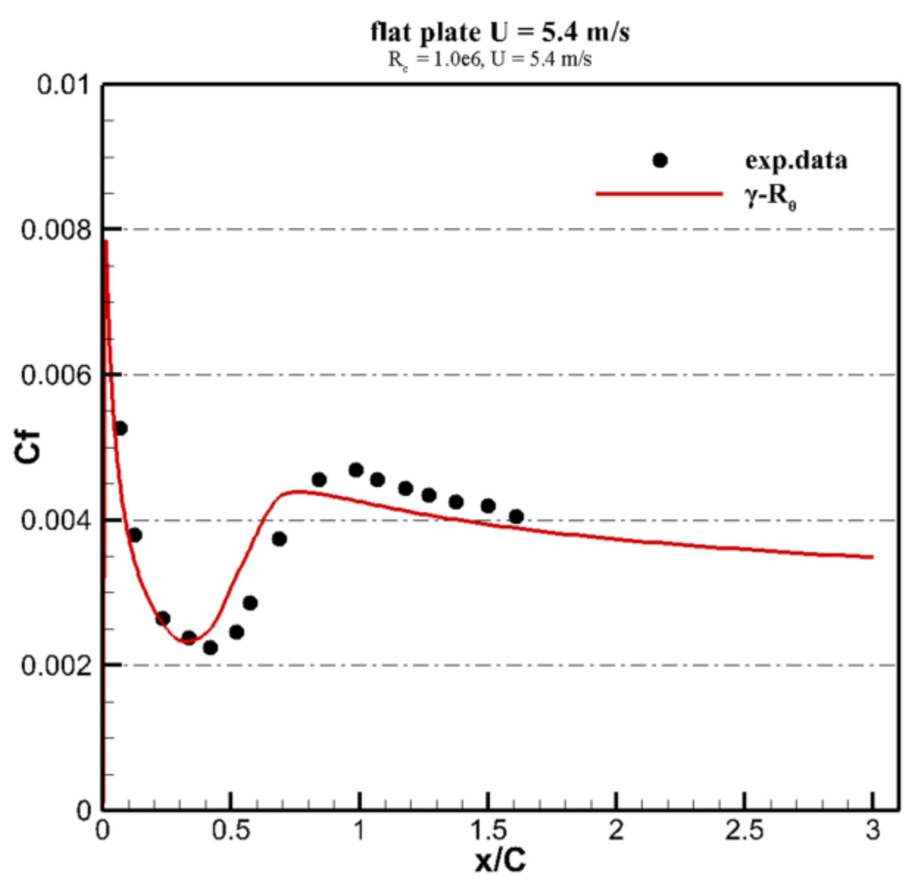
Figure 2 shows the comparison of the skin friction C f profiles predicted by the deterministic solution with the γ R θ transition model and experimental data [33,34]. The skin friction coefficient determined by the present deterministic solution could predict the transition point and developing turbulent flow well. The slight early recovery from laminar to turbulent flow and underestimation of the skin friction right after transition agreed well with previous simulation results [21].
In this study, the drag coefficient was considered as the quantity of interest of UQ. Before discussing the stochastic results of UQ, the predicted drag coefficient obtained by the deterministic solution with the originally fixed model coefficients was 0.00401.
Table 5 shows the drag coefficients predicted by the uncertainty quantification technique with the assumptions of uniform distribution of three model coefficients, ca2, ce1, and ce2, and three methods: two methods are non-intrusive polynomial chaos methods (point-collocation NIPC and non-intrusive spectral [rojection) and a Monte Carlo method with 500 simulations. The mean value and standard deviation (STD) of the drag coefficient of all three methods are presented with respect to the polynomial order.
The mean drag coefficients approached approximately 0.00413, which showed 2.9% difference compared with the deterministic solution, 0.00401. The standard deviation, which could not be predicted by the deterministic simulation, was approximately 0.00018, which was 4.4% of the mean value.
The percent errors of the mean and STD values were, respectively, 0.043% and 0.9% for point-collocation NIPC and 0.014% and 1.29% for NISP when the two methods with fifth-order were compared to those in the Monte Carlo method. 
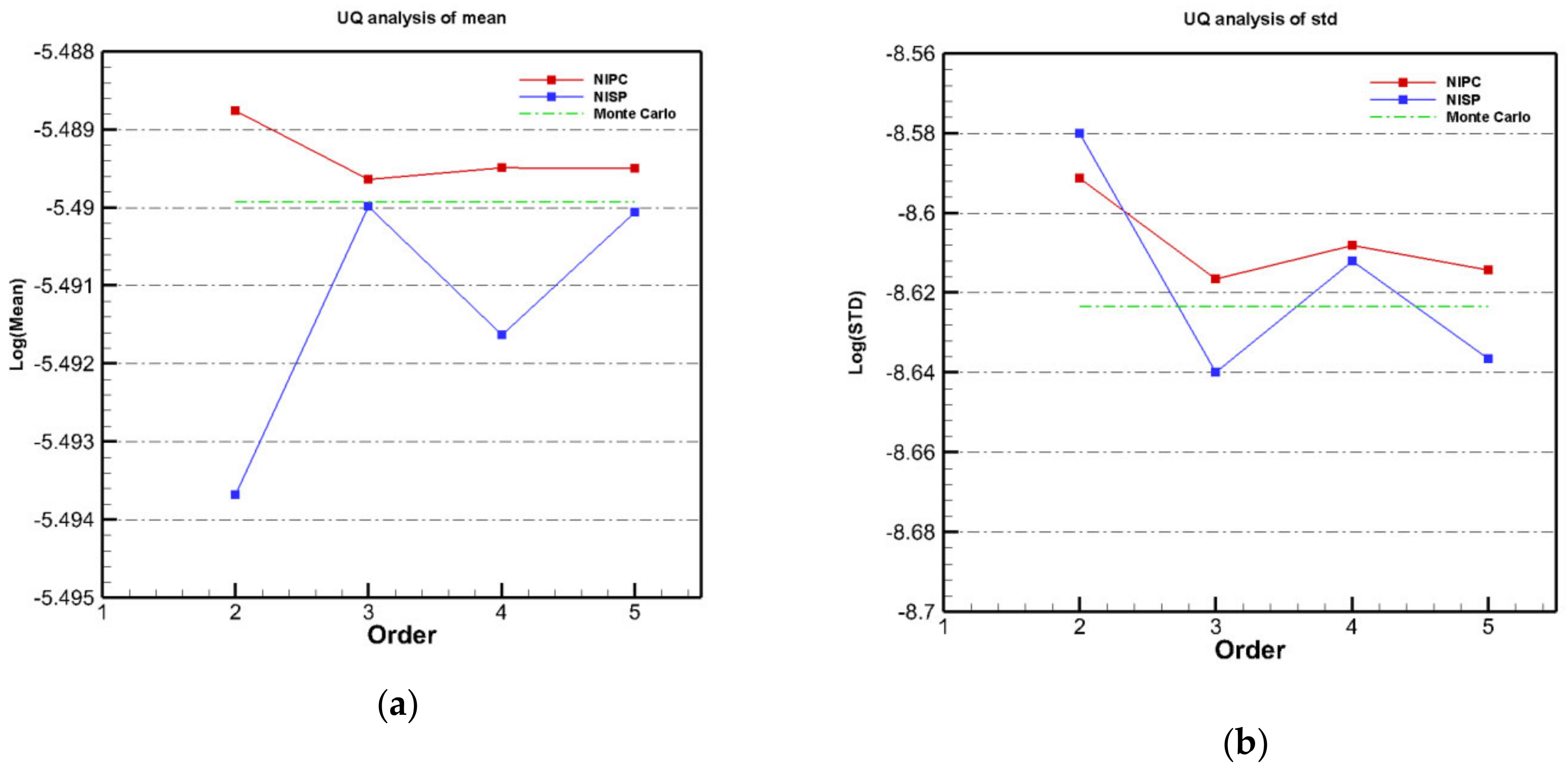
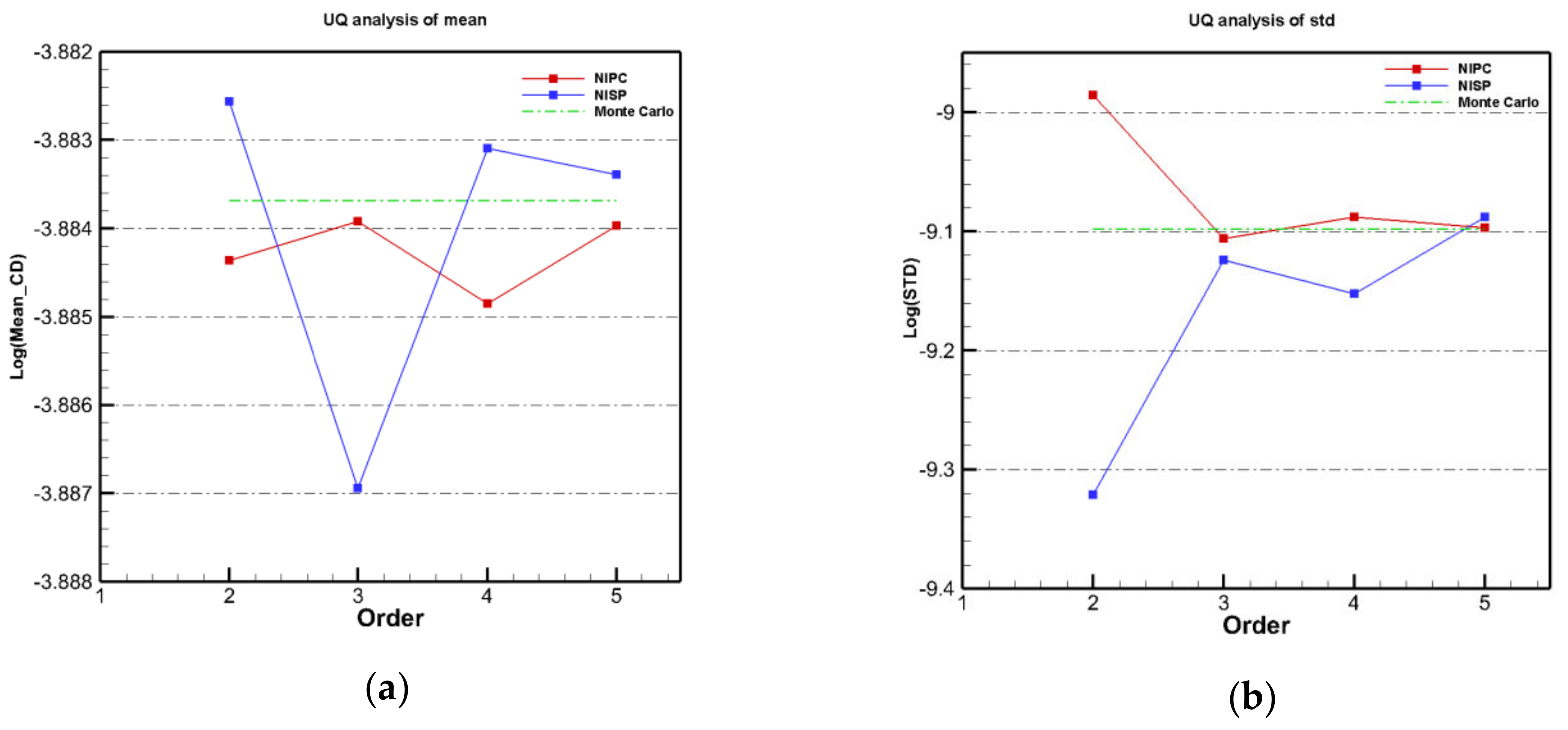
Figure 3 shows the convergence of the mean and STD of the drag coefficient according to the polynomial order of the two methods. The long dashed line is the reference value, which corresponds to the Monte Carlo results. The point-collocation NIPC showed faster convergence of the mean and STD than NISP and consistent values except for the case with second order. However, in NISP, the results of the odd number orders (third and fifth orders) are close to the Monte Carlo results and the results of the even number orders (second and fourth orders) have some discrepancies compared to the reference values.
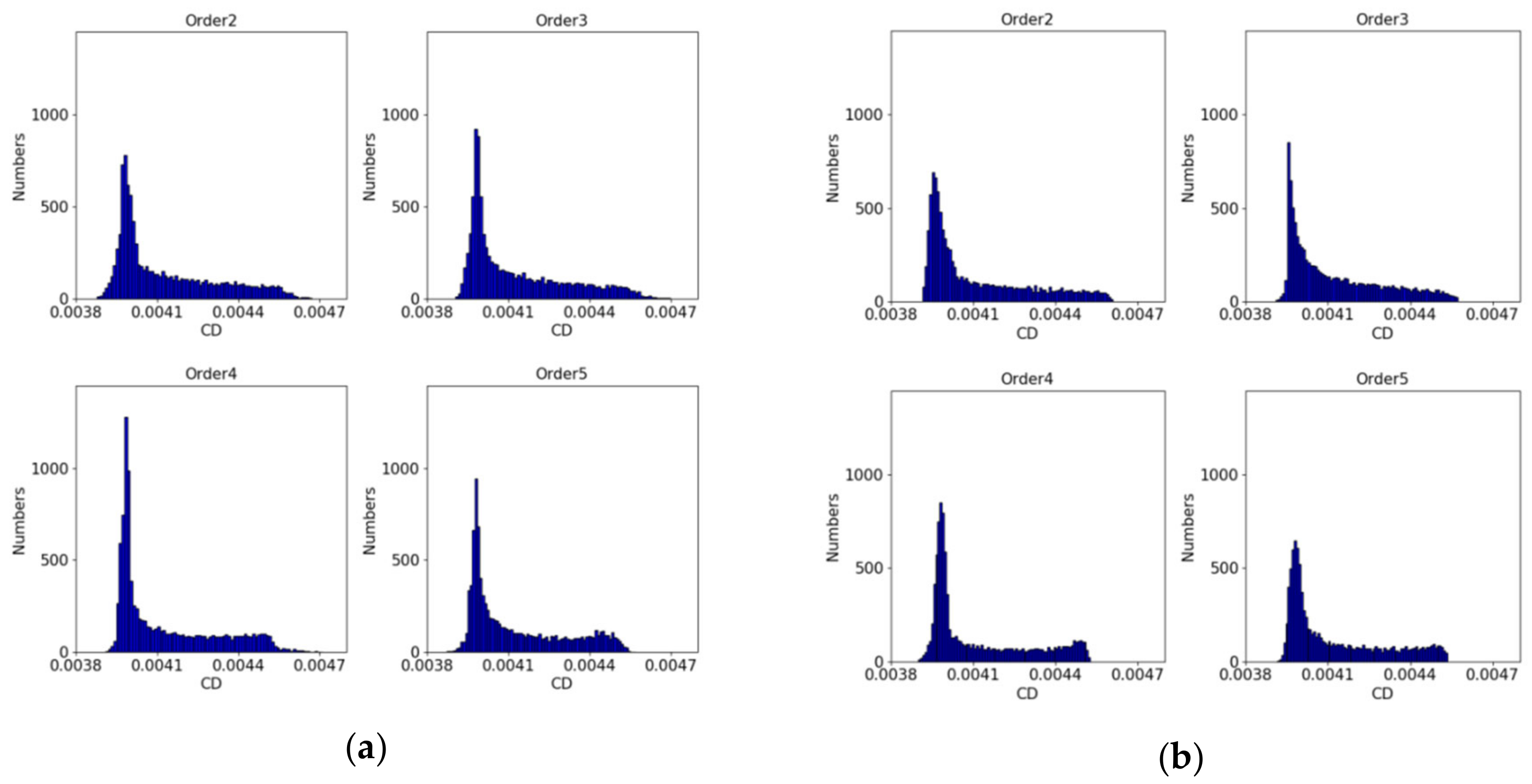
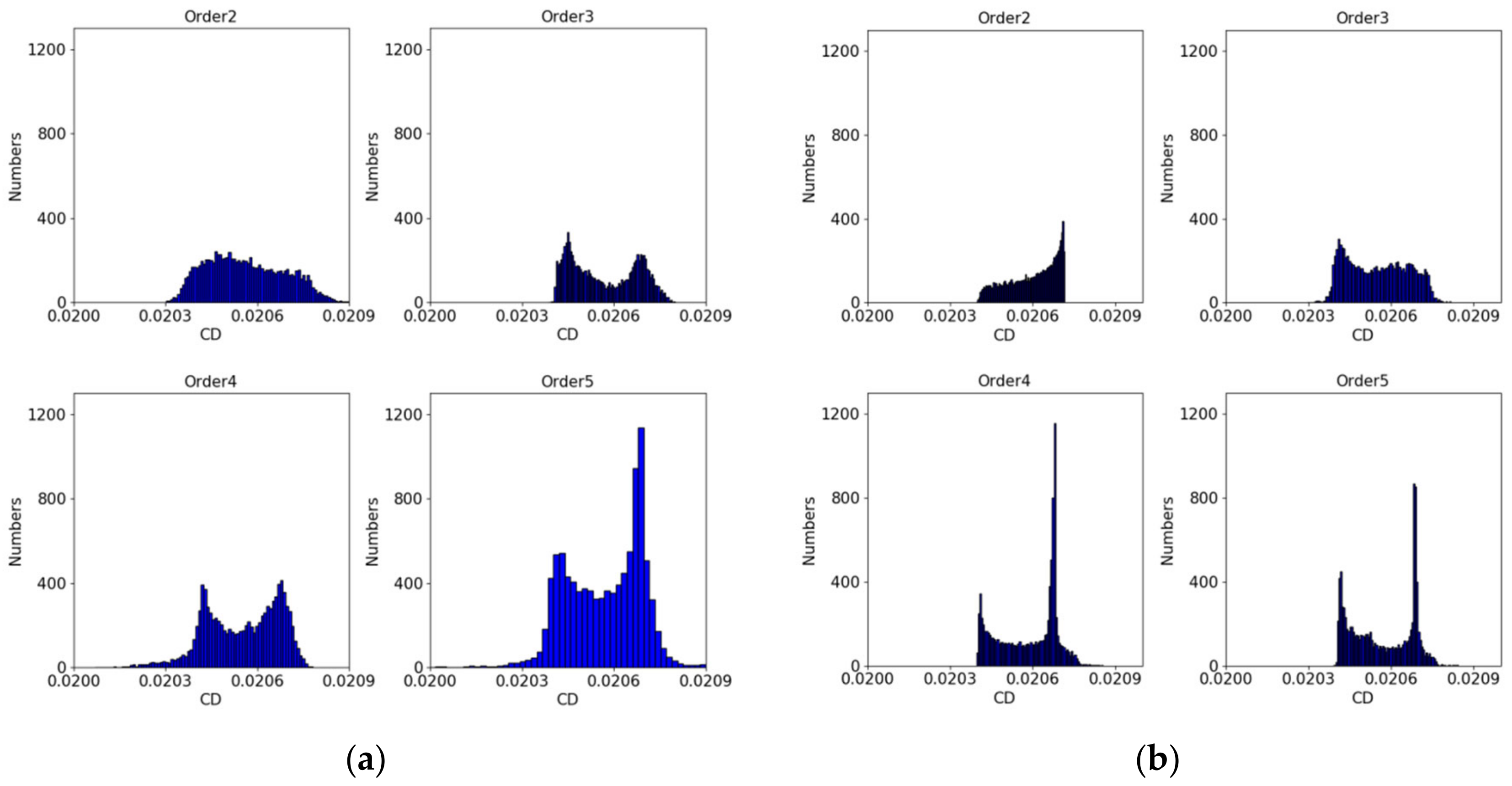
Figure 4 shows the detailed probability density function of the drag coefficient, which was generated from the calculated polynomial coefficients based on 10,000 sampling points by the Latin-Hypercube sampling method. In all cases, the peaks of the probability density function were biased toward lower values with the given interval but the value of the peak showed small differences depending on the polynomial order. As the order increased, the shape of this function had a similar pattern but there was a small difference towards higher drag coefficient values.

4.2. Transitional Flow over Aerospatiale-A Airfoil

In this section, the transitional flow around the Aerospatiale A-airfoil is presented under the conditions of the maximum lift angle of attack ( α = 13.1 ) and Re c = 2.07 × 10 6 based on the freestream velocity and chord length as shown in Figure 5. The information of the geometry and the experimental results for the Aerospatiale-A airfoil is available from the Office National d’Etudes et Recherches Ae1rospatiales F1 (ONERA F1) wind tunnel (Chaput 1997) [32]. The inflow conditions and grid system are summarized in Table 6. The turbulent intensity and eddy viscosity ratio were set to T u = 0.2 % and μ t / μ = 10 [20], respectively. The length of the upstream part and downstream part were 20c and 25c and the height of the computational domain was 30c. At the upstream and side parts, the velocity inlet boundary condition was given and, at the downstream, the Neumann boundary condition Was set for the outlet. To satisfy y + 1 for correct resolving of the turbulent boundary layer, the distance of the first mesh off the wall was 10 5 c and the growth ratio was 1.2.
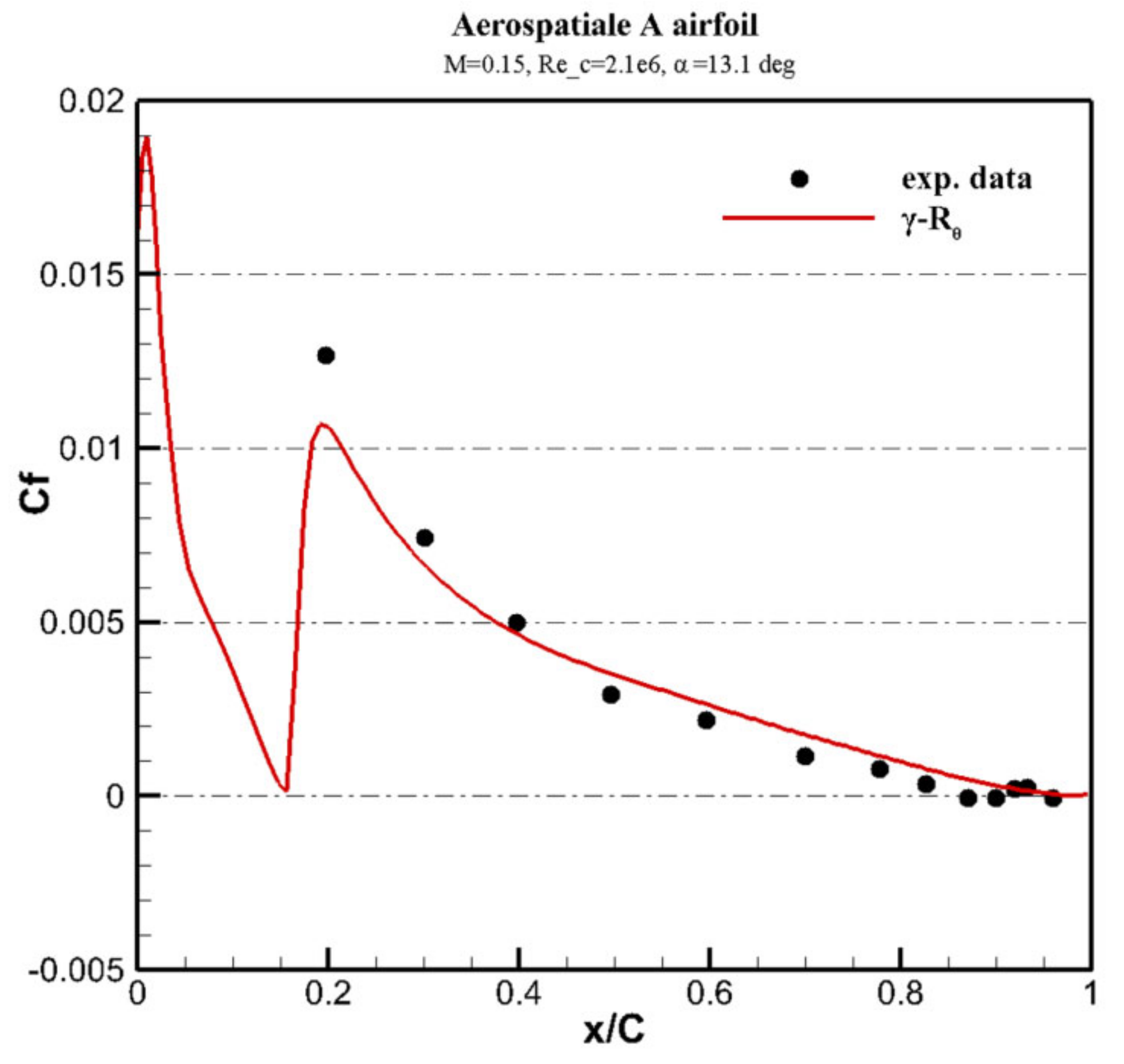
Figure 6 shows the skin friction coefficient distributions over the upper wall of the airfoil predicted by the deterministic solver with the γ R θ transition model as well as the comparison with experimental data [32]. The transition point was predicted to be between 10% and 15% of the chord length, which agreed well with other simulation results [35]. The behavior with developing turbulent flow after transition showed consistent results with experimental data.
Further, the coefficients of the drag and lift forces were calculated and compared to experimental data, F1 and F2 [32] as show in Table 7. Unfortunately, there were large discrepancies between the experimental data, F1 and F2, especially for the drag coefficient. When the measurement sensitivity of this transitional flow was considered, the present simulation showed reasonable results similar to previous simulation results [35,36]. It was confirmed that the present simulation adopts adequate methodologies and grid system.
The mean value and STD of the drag and lift coefficients of the Aerospatiale A-Airfoil were calculated using the point-collocation NIPC, NISP, and Monte Carlo methods. The number of samples of Monte Carlo was 500, which was the same as in the previous case. Table 8 shows the drag coefficient with respect to the polynomial order.
When the polynomial order is 5, the mean drag coefficient was predicted to be 0.020569 by PC-NIPC and 0.020581 by NISP. When these were compared with the deterministic solution of the original model coefficients, it was found that the drag coefficient was not as biased as in the flat plate case.
The percent errors of the mean and STD values were 0.029% and 0.09% for point-collocation NIPC and 0.03% and 0.97% for NISP when the two methods with fifth-order were compared to the Monte Carlo method. When the convergence of the drag coefficient with respect to the polynomial order was checked, the overall pattern was similar to the previous case for the drag coefficient of the flat plate flow. The mean value of the drag coefficient already converged within 0.5% (ΔCD ~ 0.0001) at the second order, whereas the STD converged after the second polynomial order as shown in Figure 7. As the polynomial order increased, the mean and STD approached the values obtained by the Monte Carlo method (long dashed line).
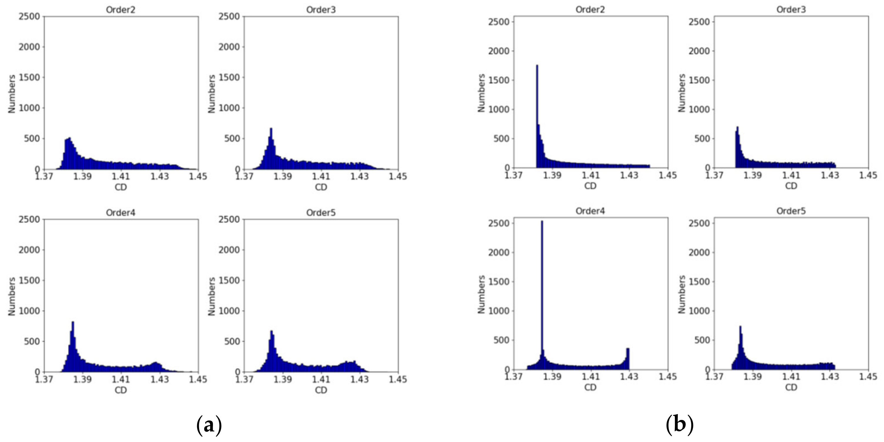
The distributions of the probability density functions of the drag coefficients are plotted with variation of the order in Figure 8. In this case, the distributions of the PDF revealed different patterns depending the adopted method and the order of the polynomial. In the case of point-collocation NIPC, the distribution of the case with second order was very different form other order cases and had similar patterns starting from the third order. NISP had a similar trend as point-collocation and the results were similar starting from the fourth-order case. Interestingly, there were two peaks in the distribution of the PDF in high-order cases for the two methods. The transitional flow simulation of Aerospatiale A-Airfoil was more sensitive to used grid, convergence criteria and the adopted scheme than the flat plate simulation. This means that the quantities of interest, such as drag and lift coefficients, were sensitive to the computational conditions (grid, convergence criteria and so on) and sampling points that were selected at the given order of polynomial. We presume that the sampling points were insufficient to resolve the exact probabilistic distribution in the lower Orders 2 and 3.
Table 9 shows the mean and STD of the lift coefficient obtained by the three methods. The mean values of all methods were predicted to be approximately 1.399, whereas the deterministic solution was 1.390.
Similar to the convergence of the drag coefficient, the mean value of the lift coefficient converged early from the second order but the STD showed a large difference when the order was 2. At the fifth order, there was a 0.85% difference in point-collocation NIPC and 0.46% in NISP as shown in Figure 9. Even though the convergence rate of point-collocation NIPC was faster than that of NISP, the accuracy at the highest order (fifth order) was higher in NISP than point-collocation NIPC. The difference between predicted and the deterministic solution value resulted because the distribution of PDF was biased toward the positive difference value, as confirmed in Figure 10.
In the lift coefficient, similar patterns of the PDF were obtained depending on the method and the order. Even though the peak of PDF was located at a lower value, the flat distributions of the lift coefficients ranged to the value of 1.43 or 1.44 in every case. This broad distribution towards a higher lift coefficient made the predicted mean lift coefficient move to a higher value than the deterministic solution.

4.3. Comparison of the Two Methods

Figure 11 describes the distribution of the PDF of point-collocation NIPC and NISP for the fifth-order polynomial and Monte Carlo method with 500 sampling points. In the case of flat plate, the peak values of the drag coefficients, 0.0041, agreed well in the three methods, NISP, PC-NIPC and Monte Carlo. This peak was located at a higher value than that (0.00401) of the deterministic solution. In the drag coefficients of Aerospatiale A-Airfoil simulation, there were two peaks in the PDF and the left peak was lower than the right one in every method. The predicted peak values in NISP and PC-NIPC methods were approximately 0.0206 with 0.03% error with that of Monte Carlo method. The pattern of the distribution of the lift coefficient in A-Airfoil simulation was similar to that of the drag coefficient in the flat plate simulation. The peak value of NISP showed smaller difference with 0.46% than that of PC-NIPC (0.86%) when compared with the Monte Carlo result. Even though the number of samplings (500) in the present work was not sufficient to get the converged solution of MC, the overall pattern distribution and the number of the peak were consistent between MC and two adopted methods. When the number of sample points for the UQ technique was considered, even though point-collocation NIPC required fewer samples than NISP (Table 3), similar accuracy and PDF as the mean and STD of the quantities of interest could be obtained. In particular, the number of random variables increased and the point-collocation NIPC was useful from a computational cost and time point of view.
Sensitivity analysis of three model coefficients, ca2, ce1, and ce2, was carried out using the Sobol index of the two methods (Table 10 and Table 11). The Sobol indices provided quantitative information regarding how much effect the corresponding random parameters had on quantities of interest. In the point-collocation NIPC and NISP methods, the most effective model coefficient was calculated as Ce1, whose Sobol index was generally over 90% in all outputs of both the flat plate and A-airfoil cases. The model coefficient Ce1 was included in the source term of the transport equation of the intermittency and was related to the Flegnth and Fonset terms. The other two variables, Ce2 and Ca2, showed similar effects on the results of less than 5% of Sobol indices. This means that more careful calibration of the model coefficient Ce1 was required compared to the other coefficients for better prediction of transitional flow.
Figure 12 displays the distribution of the skin friction coefficient from point-collocation NIPC at the fifth order. It was confirmed that the change of the model coefficients had a significant effect on the variation of the skin friction coefficient at the location of the flat plate. There was a small STD before the transition point (i.e., laminar flow region) and then a large STD after the transition (i.e., developing turbulent flow region). This means that the model closure coefficients had a large effect on the turbulent flow region of the deterministic solution.

5. Conclusions

In this study, we compared point-collocation NIPC and NISP methods for the γ Re θ transitional model [21]. Three model coefficients, Ca2, Ce1, and Ce2, were considered as multiple random inputs with the assumption of a uniform distribution with ±10% deviation. The quantities of interest were the drag and lift coefficients in transitional flow around a flat plate and Aerospatiale A-Airfoil.
The point-collocation NIPC had the advantage of having fewer samples for uncertainty quantification analysis, even though the oversampling ratio was set to 2, followed by the NISP method. It was confirmed that the point-collocation NIPC is useful when multiple random inputs are considered. Convergence with respect to the polynomial order was faster in point-collocation NIPC than NISP. In addition, the mean value of the output was obtained with a lower order than STD. This means that a higher polynomial order was necessary to obtain a converged STD. At the highest polynomial order of 5 evaluated in this study, NISP demonstrated slightly more accurate results when compared to the Monte Carlo simulation. However, the accuracy of NISP depended on whether it was an even or odd polynomial order. Through analysis of the Sobol index, the most effective model coefficient of the γ R e θ transitional model was Ce1, which is related to Flength and Foneset in the intermittency equation, by approximately over 90%.
In summary, when multiple random inputs were considered, point-collocation NIPC could provide reasonable stochastic values such as the mean and STD with fewer samples than NISP. If only one or two variables were regarded as random inputs, NISP seemed to be better at a high order.

Author Contributions

Conceptualization, T.H.N. and K.C.; Methodology, T.H.N.; Software, T.H.N.; Validation, T.H.N. and K.C.; Formal Analysis, T.H.N.; Investigation, K.C.; Resources, K.C.; Data Curation, T.H.N.; Writing-Original Draft Preparation, T.H.N.; Writing-Review & Editing, K.C.; Visualization, T.H.N. and K.C.; Supervision, K.C.; Project Administration, K.C.; Funding Acquisition, K.C.

Funding

This research was funded by the National Research Foundation of Korea Government (NRF-2016R1D1A1B03934121).

Conflicts of Interest

The authors declare no conflict of interest.

List of Symbols

c chord length (m)
Cfskin friction coefficient
M Mach number
ReReynolds number
U velocity freestream
αangle-of-attack (deg)
Tuturbulence intensity (Tu = 2 k / 3 U )
k turbulence kinetic energy (m2/s2)
μ dynamic molecular viscosity (kg.m−1.s−1)
μ t dynamic eddy viscosity (kg.m−1.s−1)
ν = μ / ρ kinematic molecular viscosity (m2/s)
ρ density (kg/m3)
εturbulence kinetic energy dissipation rate (m2/s3)
y + = y u t / ν turbulent inner layer non-dimensional coordinate

Abbreviations

CFDComputational fluid dynamics
NIPCPoint-Collocation Non-Intrusive Polynomial
NISPNon-intrusive Spectral Projection
MCMonte Carlo
PC Polynomial chaos
PDF Probability density function
UQUncertainty quantification

References

  1. Ghanem, R.; Spanos, P.D. Polynomial chaos in stochastic finite elements. J. Appl. Mech. 1990, 57, 197–202. [Google Scholar] [CrossRef]
  2. Ghanem, R. Stochastic finite elements with multiple random non-Gaussian properties. J. Eng. Mech. 1999, 26–40. [Google Scholar] [CrossRef]
  3. Ghanem, R.G. Ingredient for a general purpose stochastic finite element formulation. Comput. Meth. App. Mech. Eng. 1999, 168, 19–34. [Google Scholar] [CrossRef]
  4. Mathelin, L.; Hussaini, M.Y.; Zang, T.A.; Bataille, F. Uncertainty propagation for turbulent, compressible nozzle flow using stochastic methods. AIAA J. 2004, 42, 1669–1676. [Google Scholar] [CrossRef]
  5. Debusschere, B.J.; Naijm, H.N.; Pebay, P.P.; Knio, O.M.; Ghanem, R.G.; Maitre, O.P.L. Numerical challenges in the use of polynomial chaos representations for stochastic processes. SIAM J. Sci. Comput. 2004, 26, 698–719. [Google Scholar] [CrossRef]
  6. Reagan, M.; Najm, H.N.; Ghanem, R.G.; Knio, O.M. Uncertainty quantification in reacting flow simulations through non-intrusive spectral projection. Combust. Flame 2003, 132, 545–555. [Google Scholar] [CrossRef]
  7. Mathelin, L.; Hussaini, M.Y.; Zang, T.A. Stochastic approaches to uncertainty quantification in CFD simulations. Numer. Algorithm. 2005, 38, 209–236. [Google Scholar] [CrossRef]
  8. Wiener, N. The homogeneous chaos. Am. J. Math. 1938, 60, 897–936. [Google Scholar] [CrossRef]
  9. Wiener, N.; Wintner, A. The discrete chaos. Am. J. Math. 1943, 65, 279–298. [Google Scholar] [CrossRef]
  10. Knio, O.M.; Maitre, O.P.L. Uncertainty propagation in CFD using polynomial chaos decomposition. Fluid Dyn. Res. 2006, 38, 616–640. [Google Scholar] [CrossRef]
  11. Xiu, D.; Karniadakis, G.E. The Wiener-Askey polynomial chaos for stochastic differential equation. J. Sci. Comput. 2000, 24, 619–644. [Google Scholar]
  12. Xiu, D.; Karniadakis, G.E. Modeling uncertainty in flow simulations via generalized polynomial chaos. J. Comput. Phys. 2003, 187, 137–167. [Google Scholar] [CrossRef]
  13. Cho, J.R.; Chung, M.K. A k-ε-γ equation turbulence model. J. Fluid Mech. 1992, 237, 301–332. [Google Scholar] [CrossRef]
  14. Mayle, R.E. The role of laminar-Turbulence modeling of by-pass transition. ASME J. Turbomach. 1991, 113, 509–537. [Google Scholar] [CrossRef]
  15. Xiu, D. Numerical Methods for Stochastic Computations: A Spectral Method Approach; Princeton University Press: Princeton, NJ, USA, 2010. [Google Scholar]
  16. Hosder, S.; Walters, R.; Balch, M. Efficient Sampling for Non-Intrusive Polynomial Chaos Applications with Multiple Uncertain Input Variables. In Proceedings of the 48th AIAA/ASME/ASCE/AHS/ASC Structures, Structural Dynamics, and Materials Conference, Honolulu, HI, USA, 23–26 April 2007. AIAA 2007-1939. [Google Scholar]
  17. Hosder, S.; Walters, R.; Perez, R. A Non-Intrusive Polynomial Chaos Method for Uncertainty Propagation in CFD Simulations. In Proceedings of the 44th AIAA Aerospace Sciences Meeting and Exhibit, Reno, NV, USA, 9–12 January 2006. AIAA 2006-891. [Google Scholar]
  18. Loeven, G.J.A.; Witteveen, J.A.S.; Bijl, H. Probabilistic Collocation: An Efficient Non-Intrusive Approach for Arbitrarily Distributed Parametric Uncertainties. In Proceedings of the 45th AIAA Aerospace Sciences Meeting and Exhibit, Reno, NV, USA, 8–11 January 2007. AIAA 2007-317. [Google Scholar]
  19. Platteeuw, P.D.A.; Loeven, G.J.A.; Bijl, H. Uncertainty quantification applied to the k-epsilon model of turbulence using the probabilistic collocation model. In Proceedings of the 49th AIAA/ASME/ASCE/AHS/ASC Structures, Structural Dynamics and Materials Conference, Schaumburg, IL, USA, 7–10 April 2008. [Google Scholar]
  20. Schaefer, J.; West, T.; Hosder, S.; Rumsey, C.; Carlson, J.; Kleb, W. Uncertainty quantification of turbulence model coefficients for transonic wall-bounded flow. AIAA J. 2017, 55, 195–213. [Google Scholar] [CrossRef]
  21. Langtry, R.B.; Menter, F.R. Correlation-based transition modeling for unstructured parallelized computational fluid dynamics Codes. AIAA J. 2009, 47, 2894–2906. [Google Scholar] [CrossRef]
  22. Menter, F.R. Two-equation eddy-viscosity turbulence models for engineering application. AIAA J. 1994, 32, 1598–1605. [Google Scholar] [CrossRef]
  23. Drela, M.; Giles, M.B. Viscous-inviscid analysis of transonic and low Reynolds number airfoils. AIAA J. 1987, 25, 1347–1355. [Google Scholar] [CrossRef]
  24. Rumsey, C.L.; Gatski, T.B.; Ying, S.X.; Bertelru, A. Prediction of high-lift flows using turbulent closure models. AIAA J. 1998, 36, 765–774. [Google Scholar] [CrossRef]
  25. Sullivan, T.J. Introduction to Uncertainty Quantification; Springer: Cham, Switzerland, 2015; Volume 63. [Google Scholar]
  26. Bijl, H.; Lucor, D.; Mishra, S.; Schwab, C. Implementation of Intrusive Polynomial Chaos in CFD Codes and Application to 3D Navier-Stokes. In Uncertainty Quantification in Computational Fluid Dynamics; Springer: Cham, Switzerland, 2013. [Google Scholar]
  27. Perez, R.; Walters, R. An Implicit Compact Polynomial Chaos Formulation for the Euler Equations. In Proceedings of the 43rd AIAA Aerospace Sciences Meeting and Exhibit, Reno, NV, USA, 10–13 January 2005. AIAA 2005-1406. [Google Scholar]
  28. Feinberg, J.; Langtangen, H.P. Chaospy: An open source tool for designing methods of uncertainty quantification. J. Comput. Sci. 2015, 11, 46–57. [Google Scholar] [CrossRef]
  29. NISP Details. Available online: http://atoms.scilab.org/toolboxes/NISP/2.1 (accessed on 29 September 2009).
  30. Fu, S.; Wang, L. Progress in turbulence/transition modeling. Adv. Mech. 2007, 37, 409–416. [Google Scholar]
  31. Zarmehri, A. CFD with OpenSource Software: γ − Rθ Transitional Turbulence Model Tutorial; Chalmers University of Technology: Gothenburg, Sweden, 19 November 2012; pp. 1–24. [Google Scholar]
  32. Schmidt, S.; Thiele, F. Detached eddy simulation of flow around A-airfoil. Flow Turbul. Combust. 2003, 71, 261–278. [Google Scholar] [CrossRef]
  33. Savill, A.M. One-Point Closures Applied to Transition. In Turbulence and Transition Modeling; Hallback, M., Ed.; Kluwer: Dordrecht, The Netherlands, 1996; pp. 233–268. [Google Scholar]
  34. Rumsey, C.L. Turbulence Modeling Resource. Available online: http://turbmodels.larc.nasa.gov/ (accessed on 13 February 2009).
  35. Ke, J.; Edwards, J.R. Numerical simulations of turbulent flow over airfoils near and during static stall. J. Aircr. 2017, 54, 1960–1978. [Google Scholar] [CrossRef]
  36. Goldberg, U.C.; Batten, P.; Peroomian, O.; Chakravathy, S. The R-γ transition prediction model. Int. J. Comput. Flud Dyn. 2015, 29, 26–39. [Google Scholar] [CrossRef]
Figure 1. Computational mesh for the flat plate.
Applsci 09 01407 g001
Figure 2. Skin friction coefficient distribution with the original formulation over the flat plate.
Applsci 09 01407 g002
Figure 3. The mean and standard deviations of the drag coefficient of the three methods for Orders 2–5: (a) mean value; and (b) standard deviation.
Applsci 09 01407 g003
Figure 4. PDF analysis of the drag coefficient: (a) point-collocation non-intrusive polynomial chaos; and (b) non-intrusive spectral projection.
Applsci 09 01407 g004
Figure 5. Computational mesh for Aerospatiale A-airfoil.
Applsci 09 01407 g005
Figure 6. Skin friction coefficient distribution for the original formulation over Aerospatiale A-airfoil.
Applsci 09 01407 g006
Figure 7. The mean and standard deviations of the drag coefficient of the three methods for Orders 2–5: (a) mean value; and (b) standard deviation.
Applsci 09 01407 g007
Figure 8. PDF analysis of the drag coefficient (CD): (a) point-collocation non-intrusive polynomial; and (b) non-intrusive spectral projection.
Applsci 09 01407 g008
Figure 9. The mean and standard deviations of the lift coefficient of the three methods for Orders 2–5: (a) mean value; and (b) standard deviation.
Applsci 09 01407 g009
Figure 10. PDF analysis of the lift coefficient (CL): (a) point-collocation non-intrusive polynomial; and (b) non-intrusive spectral projection.
Applsci 09 01407 g010
Figure 11. The distributions of the PDF at the fifth order of NIPC, NISP, and Monte Carlo (CL): (a) CD of flat plate; and (b) CD of A-airfoil, and (c) CL of A-airfoil.
Applsci 09 01407 g011
Figure 12. Variation of the skin friction coefficient of the upper surface of the A-airfoil for the point-collocation NIPC method.
Applsci 09 01407 g012
Table 1. The sensitivity analysis of each model coefficient.
CoefficientCD of Lower Boundary (−10%)CD of Upper Boundary (10%)Difference Percent (%)
Ca20.003910.004104.60
Ce10.003730.0042111.4
Ce20.003970.004062.22
Ca10.003950.004021.74
Cα0.004010.004050.99
δ γ 0.003990.004010.49
σ θ t 0.003890.003920.76
C θ t 0.004020.003981.0
Table 2. The uniform distributions of the three model coefficients ±10% deviation.
CoefficientOriginal ValueLower Boundary (−10%)Upper Boundary (10%)
Ca20.060.0540.066
Ce11.00.91.1
Ce250.045.055.0
Table 3. The total numbers of selected points for Monte Carlo, NIPC, and NISP for three chosen points (n is the dimension and p is the order of stochastic computation).
n = 3Monte Carlo
MC
Point-Collocation NIPCSpectral Project
NISP
Order- 2 ( n + p ) ! n ! p ! ( p + 1 ) n
2 2027
35004064
4 70125
5 112216
Table 4. Information regarding the inflow conditions and grid system for flow over a flat plate.
Inflow Condition U 5.4 m/s
T u 3.3%
μ t / μ 10.0
Grid System(Lx,Ly)(3.2c,1.0c)
(Nx,Ny)(230,100)
Re L 1 × 10⁶
(L = 0.3 m)
Table 5. The mean and standard deviation of the drag coefficient values for flat plate.
OrderMean_NIPCSTD_NIPCMean_NISPSTD_NISPMean_MCSTD_MC
20.004132980.00018570.004112690.00018780.0041281390.00017982
30.004129330.00018110.004127910.0001769
40.004129970.00018260.004121130.0001819
50.004129920.00018150.004127580.0001775
Table 6. Information about the inflow conditions and grid system for flow over Aerospatiale A-airfoil.
Inflow Condition U 32.8 m/s
T u 0.2%
μ t / μ 10.0
α 13.1
Grid System(Lx,Ly)(45c,30c)
(Nx,Ny)(350,120)
Re c 2.07 × 10 6
Table 7. Lift and drag at α = 13.1
Model C L C D
γ R θ 1.3900.0206
F1 exp1.5620.0208
F2 exp1.5150.0308
Table 8. The mean and standard deviation of the drag coefficient (CD) values for A-airfoil.
OrderMean_NIPCSTD_NIPCMean_NISPSTD_NISPMean_MCSTD_MC
20.0205610.00012520.0205980.00008950.020574890.0001119
30.0205700.0001110.0205080.0001090
40.0205510.0001130.0205870.0001060
50.0205690.0001120.0205810.0001130
Table 9. The mean and standard deviation values of the lift coefficient (CL) for A-airfoil.
OrderMean_NIPCSTD_NIPCMean_NISPSTD_NISPMean_MCSTD_MC
21.399990.0177301.3975220.0173211.3991550.016661
31.399550.0168211.3998020.016343
41.399490.0169691.3985510.017026
51.399670.0168041.3995070.016583
Table 10. Sobol index of three model coefficients for point-collocation NIPC.
Sobol IndexCa2Ce1Ce2
CD Flat plate0.019340.9830.01955
CD A-airfoil0.322560.89630.15859
CL A-airfoil0.053470.97930.03839
Table 11. Sobol index of three model coefficients for NISP.
Sobol IndexCa2Ce1Ce2
CD Flat plate0.00340.99450.0022
CD A-airfoil0.02870.95540.0281
CL A-airfoil0.000240.99990.000234

