Vibration-Induced Pressures on a Cylindrical Structure Surface in Compressible Fluid

Featured Application

This study established a new approach for calculating the effect of vibration-induced pressures on cylindrical thin-walled structures. Such a method will benefit the design of cylindrical thin-walled structures subjected to wind loads, earthquakes, etc. Structural designers can use the approach to evaluate the structural effects of vibrating air or fluid.

Abstract

This paper unprecedentedly addresses the effect of vibrations of a cylindrical structure on dynamic pressures in a compressible and incompressible fluid situation. To obtain analytical solutions, the density of the fluid is simplified as a constant, but the rates of the density with respect to time and to space are considered as a dynamic and time-dependent function. In addition, the low velocity of the vibration is taken into account so the lower order terms are negligible. According to the assumption that the vibration at the boundary of the structure behaves as a harmonic function, some interesting and new analytical solutions can be established. Both analytical solutions in the cases of the compressible and incompressible fluid are rigorously verified by the calibrated numerical simulations. New findings reveal that, in the case of the incompressible fluid, dynamic pressure at the surface of the cylindrical shell is proportional to the acceleration of the vibration, which acts like an added mass. In the case of the compressible fluid, the pressure at the surface of the cylindrical structure is proportional to the velocity of the vibration, which acts as a damping. In addition, the proportional ratio is derived as $\rho c$.

1. Introduction

In recent years, owing to the large demand for civilian buildings, ocean engineering, military structures, and membrane structures [1,2], many large-span structures have been widely designed for public uses [3,4,5]. It is well known that those structures are generally light and flexible so they are sensitive to dynamic loads, such as wind loads, seismic loads, etc. [6]. There are several examples [7,8,9] in which fluid pressure induced by the vibration of light and flexible structures has a significant effect on the mechanical system. However, the prediction of the fluid pressure induced by the vibration is very difficult; and there are very few pertinent investigations in the open literature. Due to the lack of understanding in this field, it is necessary to embark on studies, including experimental, theoretical, and numerical simulation studies [10,11,12].

Based on the potential flow theory [13,14] and the hypothesis that the vibration mode of a structure can be a sinusoidal function shape, Minami [15] deduced a significant result that the added mass of a planar membrane in a rectangle is 0.68 divided by the mass ratio, $m/\rho l$. Actually, his conclusion only fulfilled the 1-D condition. Kubenko, Dzyuba [16] proposed a new method to investigate the behavior of an elastic shell submerged in an unbounded fluid. In his paper, the fluid was assumed to be an elastic medium, and some analytical solutions written as a Fourier series were proposed. Several publications exist that investigated VIV (vortex-induced vibration) problems. Sorokin et al. [17] studied flow-induced vibration of a cylindrical shell conveying a compressible fluid. Chung [18] addressed a new approach to estimate the pressure of a circular shell beneath a free surface.

Mancinellli and Brocchini [14] carried out an experimental investigation of wave-induced flow around a cylinder in different conditions with several Keulegan-Carpenter ratios and Reynolds numbers. In Kaiser Calautit’s work [19], numerical analysis of several wind towers located on the same building was conducted following the verification of a benchmark model against the wind tunnel data. Some new findings were produced via experiments, but those findings did not include discussion via theoretical analysis.

Unfortunately, in the papers presented above, the incompressible fluid hypothesis was mostly taken into account [20,21], which can simplify the mathematical difficulty in the analytical solution, but also changes the physical rules of the FSI problems [22,23,24,25]. In addition, very few studies were devoted to vibrations of a cylindrical shell.

Based on the reasons above, this paper is the first to consider a cylindrical structure vibrating in the radius direction in both compressible and incompressible fluid [26,27,28]. Additionally, some analytical solutions were obtained. In addition, a new mathematical model about the damping ratio of the cylindrical shell vibrating in the fluid was derived and validated. This study enables a novel analytical prediction that can be practically utilized in the design and analysis of cylindrical shell structures interacting with wind loads, earthquakes, blast loading, and so on. This new mathematical technique can be extended to the other research fields. The rest of this study is organized as follows: The governing equations are presented in Section 2. In Section 3, the numerical verifications are investigated and discussed, and finally a summary and conclusions are presented in Section 4.

2. Governing Equations

Based on the inviscid fluid consideration, there is an assumption of $p=c^2\rho$, where $p$, $c$, and $\rho$ denotes the static pressure, the sound speed, and the density of the fluid, respectively. The fluid–structure interaction equation can be employed below [29], relying on the assumption that the amplitude of the cylindrical structure vibrating in the radius direction is relatively small compared to its radius. The geometry model is shown in Figure 1. Considering the rotationally symmetric deformation of this structure [30,31,32], the dynamic pressure on the boundary of the fluid affects the structure simultaneously. The governing equations include both the structure dynamics equation as Equation (1) [33,34] and the fluid dynamic equation as Equation (2) [35,36,37], namely:

$$m\frac{{\partial }^{2}U}{{\partial }^{2}t}+k\cdot {\nabla }^{4}U+\Delta p=0$$

(1)

$$\{\begin{array}{l}\frac{\partial \rho }{\partial t}+\frac{\partial \rho u}{\partial r}+\frac{\rho u}{r}=0\\ \frac{\partial u}{\partial t}+u\frac{\partial u}{\partial r}+\frac{c^2}{\rho }\frac{\partial \rho }{\partial r}=0\end{array}$$

(2)

Equation (1) is the typical structural dynamic mechanical equation, where $m$ is the areal density of the structure, $U$ is the displacement, $k$ is the bending stiffness, and $\Delta p$ is the pressure of the flow field boundary acting upon the structure. The initial conditions can be written as follows:

$${U|}_{t=0}=0,{\frac{\partial U}{\partial t}|}_{t=0}=u_s(0)$$

(3)

Equation (2) is the fluid control equation, which is also called the Naiver-stokes equation. The first equation of Equation (2) is the mass conservation equation and the second one is the conservation of momentum equation. In Equation (2), $\rho$ is the fluid density, $p$ the static pressure in the fluid field, $c$ is the sound speed, and $u$ is the fluid velocity generated by the vibration of the boundary. On introducing the symbol:

$$\frac{\partial U}{\partial t}=u_s(t)=u$$

(4)

The boundary conditions can be written as follows:

$${u|}_{r=r_s}=u_s(t),{p|}_{r=R}=p_0{,u|}_{r=R}=0$$

(5)

where $r_s$ expresses the boundary of the fluid and is a function of the time, thus:

$$r_s=r_s(0)+U$$

(6)

On the assumption that the amplitude is very small compared to the radius, $r_s$, $r_s$ can be considered as a constant value. The initial conditions can be written as shown below (Equation (7)):

$${u|}_{t=0}=0,{\rho |}_{t=0}={\rho }_0,{p|}_{t=0}=p_0$$

(7)

2.1. Solution of the Compressive Fluid

It can be assumed that the velocity can be a harmonic function with a frequency of $\omega$, so it can be written as:

$$\frac{{\partial }^{2}u}{\partial t^2}=-{\omega }^{2}u$$

(8)

Meanwhile, based on the physical property of the fluid, the density change is very small, but the rate of the density with respect to time or respect to space may not be small. As a matter of fact, the smaller the change of the density, the larger the change of the pressure according to the state equation of fluid. Therefore, in this paper, the density is assumed to be a constant value, ${\rho }_o$, and the rate of the density with respect to time or to space are variables. From the second term of Equation (2), it can be transformed to Equation (9):

$$\Delta \rho =\rho -{\rho }_0=-\frac{{\rho }_o}{c^2}{\displaystyle {\int }_r^{\infty }\frac{\partial u}{\partial t}}dr+\frac{{\rho }_o}{2}\frac{u^2}{c^2}$$

(9)

From Equation (3), it can be seen that the changes in density or pressure come from two sources: The change of the velocity with respect to time or to space. By neglecting the second term of Equation (3) and substituting another term into the continuous equation, the following equation can be obtained (Equation (10)):

$$-\frac{{\rho }_o}{c^2}{\displaystyle {\int }_r^{\infty }\frac{{\partial }^{2}u}{\partial t^2}}dr+{\rho }_o\frac{\partial u}{\partial r}+\frac{{\rho }_{o}u}{r}=0$$

(10)

Afterwards, Equation (3) can be transformed after being divided by the density, ${\rho }_o$:

$$-\frac{{\omega }^2}{c^2}{\displaystyle {\int }_r^{\infty }u}dr+\frac{\partial u}{\partial r}+\frac{u}{r}=0$$

(11)

Furthermore, the equation can be simplified by taking the derivative on both sides of Equation (11):

$$\frac{{\partial }^{2}u}{\partial r^2}+\frac{1}{r}\frac{\partial u}{\partial r}+(\frac{{\omega }^2}{c^2}-\frac{1}{r^2})u=0$$

(12)

By letting $s=\omega \cdot r/c$, the above equation can be simplified as Equation (13), finally:

$$s^2\frac{{\partial }^{2}u}{\partial s^2}+s\frac{\partial u}{\partial s}+(s^2-1)u=0$$

(13)

Equation (13) is the classical Bessel function [38,39]; the general solution can be derived as:

$$u=A\cdot J_1(s)+B\cdot Y_1(s)$$

(14)

where $A$, $B$ is an arbitrary function with respect to time. $J_1(s)$, $Y_1(s)$ is the first and second order Bessel function, respectively. The coefficient of $A$, $B$ can be confirmed via the boundary condition:

$$\{\begin{array}{l}{u_s(t)|}_{r=r_s}=A\cdot J_1(s_{r_s})+B\cdot Y_1(s_{r_s})\\ 0=A\cdot J_1(s_R)+B\cdot Y_1(s_R)\end{array}$$

(15)

If the radius of the boundary is $R\to \infty$, the second boundary condition will be satisfied naturally as $J_1(s_R)$, $Y_1(s_R)$ tends to 0. In this case, it is reasonable to assume $u$ as a harmonic function with a frequency of $\omega$ as well, so that:

$$A=C\cdot \cos (\omega t+\phi ),B=C\cdot \sin (\omega t+\phi )$$

(16)

where, $C$, $\phi$ are the coefficients which express the amplitude and phase angle, respectively. By considering the velocity as a harmonic function, $u_s(t)=D\cdot \sin (\omega t)$ can be obtained, where $D$ is the amplitude of the vibration. Additionally, the boundary condition can be written as Equation (17) below by submitting Equation (16) to Equation (15). The coefficients of $C$ and $\phi$ can thus be confirmed:

$$C\cdot (\cos (\omega t+\phi )J_1(s_r)+\sin (\omega t+\phi ))Y_1(s_r)=D\cdot \sin (\omega t)$$

(17)

2.2. Analyses of the Velocity

The solution of Equation (17) can be simplified as follows via trigonometric function theory:

$$C\sqrt{J_1^2(s_r)+Y_1^2(s_r)}\sin (\omega t+\phi +\varphi )=D\cdot \sin (\omega t)$$

(18)

where $s_r=\frac{\omega }{c}{r}_r$, $\tan (\varphi )=\frac{J_1(s_r)}{Y_1(s_r)}$. So, it can be concluded that by solving Equation (18) above:

$$C=\frac{D}{\sqrt{J_1^2(s_r)+Y_1^2(s_r)}},\phi =-\varphi =-\arctan (\frac{J_1(s_r)}{Y_1(s_r)})$$

(19)

Moreover, the Bessel functions have the following asymptotic forms for large arguments, $s$:

$$\{\begin{array}{l}{J}_1(s)=\sqrt{\frac{2}{\pi }}\frac{\cos (s-\frac{3}{4}\pi )}{\sqrt{s}}\\ Y_1(s)=\sqrt{\frac{2}{\pi }}\frac{\sin (s-\frac{3}{4}\pi )}{\sqrt{s}}\end{array}$$

(20)

At last, the analytical solution of the velocity can be concluded using the previous relationship:

$$u=\frac{D}{\sqrt{J_1^2(s_r)+Y_1^2(s_r)}}\sqrt{\frac{c}{\omega }\frac{2}{\pi }}\frac{\cos (\omega (t-\frac{r}{c})+\phi +\frac{3}{4}\pi )}{\sqrt{r}}$$

(21)

According to Equation (21), the vibration of the boundary at time $t_0$ will be propagated to the location, $r=ct$, over time $t$ and the amplitude will decrease by the decreasing rate of $\raisebox{1ex}{$1$}\!\left/ \!\raisebox{-1ex}{$\sqrt{r}$}\right.$.

2.3. Analyses of the Pressure

As for the pressure analysis, it is known from Equation (9) that the pressure contributed by acceleration with respect to time is:

$$\Delta P=-{\rho }_o{\displaystyle {\int }_r^{\infty }\frac{\partial u}{\partial t}}dr$$

(22)

The Bessel function has the following asymptotic forms for large arguments, $s$:

$${\displaystyle \int J_1(r)}dr=-J_0(r),{\displaystyle \int Y_1(r)}dr=-Y_0(r),\underset{r\to \infty }{\lim }{J}_1(r)=0,\underset{r\to \infty }{\lim }{Y}_1(r)=0,$$

(23)

Therefore:

$$\Delta P={\rho }_{o}c\frac{D}{\sqrt{J_1^2(s_r)+Y_1^2(s_r)}}[\cos (\omega t+\phi +\frac{\pi }{2})J_0(s)+\sin (\omega t+\phi +\frac{\pi }{2})Y_0(s)]$$

(24)

where the value of $s$, $\phi$ is the same as in Section 2.2 above. If $s$ is large, the following statement will be true:

$$\{\begin{array}{l}{J}_1(s)=\sqrt{\frac{2}{\pi }}\frac{\cos (s-\frac{1}{4}\pi )}{\sqrt{s}}\\ Y_1(s)=\sqrt{\frac{2}{\pi }}\frac{\sin (s-\frac{1}{4}\pi )}{\sqrt{s}}\end{array}$$

so, the simplest solution may be got, finally,

$$\Delta P={\rho }_{o}c\frac{D}{\sqrt{J_1^2(s_r)+Y_1^2(s_r)}}\sqrt{\frac{c}{\omega }\frac{2}{\pi }}\frac{\cos (\omega (t-\frac{r}{c})+\phi +\frac{3\pi }{4})}{\sqrt{r}}={\rho }_{o}c\cdot u.$$

(25)

It can be derived from Equation (25) that the pressure is proportional to the velocity of the vibration and the proportion is a product of the density and sound speed. In addition, it is a large value compared to the pressure contributed from migration acceleration, $\raisebox{1ex}{$1$}\!\left/ \!\raisebox{-1ex}{$2$}\right.{\rho }_o{u}^2$. That is the mean, neglecting migration acceleration as done in the solution of Section 2.2, is reasonable.

2.4. Incompressible Fluid Solution

For comparison, it is necessary to consider the case of vibration in the incompressible fluid situation. The control equation can be listed as follows:

$$\{\begin{array}{l}m\frac{{\partial }^{2}U}{{\partial }^{2}t}+k\cdot U+\Delta p=0\\ \frac{\partial u}{\partial r}+\frac{u}{r}=0\\ \frac{\partial u}{\partial t}+u\frac{\partial u}{\partial r}+\frac{1}{{\rho }_o}\frac{\partial p}{\partial r}=0\end{array}.$$

(26)

where the symbols are the same as in Section 2.1. The boundary condition in the structural equation in this case is the same as Section 2.1, while the boundary condition in the fluid aspect is:

$$\{\begin{array}{l}{u|}_{r=r_s}=u_s(t)\\ {p|}_{r=R}=p_0\end{array}$$

(27)

The following solution can be concluded according to the continued equation of Equation (26) combined with the boundary condition of ${u|}_{r=r_s}=u_s(t)$:

$$u(r,t)=\frac{r_s}{r}{u}_s(t)$$

(28)

Also, the general solution of pressure can be obtained below from the momentous equation of Equation (26) by substituting Equation (28) into it:

$$p(r)=-{\rho }_0\frac{\partial u_s}{\partial t}\ln (R/r)-\frac{1}{2}\frac{u_s^2}{r^2}+C$$

(29)

At last, the specific solution of this case may be deduced as follows combined with the boundary condition of ${p|}_{r=R}=p_0$:

$$\Delta p=p-p_0={\rho }_0{r}_s\frac{\partial u_s}{\partial t}\cdot \ln (\frac{R}{r})+\frac{1}{2}{\rho }_0{u}_s^2\frac{r_s^2}{r^2}$$

(30)

Generally speaking, $R$ is a large value and the vibration acceleration, $\partial u_s/\partial t$, may be of the same order with a magnitude of $u_s$. Therefore, the second term in the specific solution of Equation (30) can be neglected and the approximate result can be derived as the following statement:

$$\Delta p={\rho }_0{r}_s\frac{\partial u_s}{\partial t}\cdot \ln (\frac{R}{r})$$

(31)

2.5. Discussion

There are some significant differences between the solution of Equations (25) and (31). As for the case of an incompressible fluid, the pressure is proportional to the boundary acceleration and it has a logarithmic relationship with the length of the flow field, which implies that the radius of the boundary has a significant effect on the pressure result. In addition, after substituting Equation (31) into Equation (1), it was found that the effect of pressure is equivalent to the effect of added mass. It is remarkable that if the radius of the boundary becomes extremely large (mostly it will be in the CFD solution), the pressure on the boundary surface becomes very large as well. This characteristic can result in unsolvable difficulties in fluid–structure interaction problems using CFD methods.

As for the case of the compressible fluid case, according to the solution, $\Delta p={\rho }_{o}c\cdot u$, it can be concluded that the pressure is proportional to the velocity of the boundary, and the proportional ratio is the product of the sound speed and the density. In this case, the effect of the pressure is equivalent to the viscous damping, and the damping coefficient is a constant value.

From the point of view of a physical sense, over time, $\Delta t$, the amount of fluid affected by the structure is $\pi [{(r_s+u_s\Delta t)}^2-r_s^2)]$, whilst, the region it can reach is $\pi [{(r_s+c\Delta t)}^2-r_s^2]$. Thus when $\Delta t\to 0$, the air compression ratio is:

$$\underset{\Delta t\to 0}{\lim }\frac{\pi [{(r_s+u_s\Delta t)}^2-r_s^2)]}{\pi [{(r_s+c\Delta t)}^2-r_s^2]}=\frac{u_s}{c}$$

(32)

Plus, the air compression modulus [40] is ${\rho }_o{c}^2$, and the pressure of compression air can be calculated as follows according to Hoke’s law:

$$p=c^2\cdot \frac{u_s}{c}={\rho }_{o}c\cdot u_s$$

(33)

which is identical to Equation (25).

3. Numerical Verification

Based on the preceding analysis, two simulations with a semi-circular shell submerged in unbounded fluid were calculated by CFD analysis using commercial computer code, ANSYS (release 18.0). The CFD model has an identical shell geometry, boundary conditions, and material properties as those used in the theoretical analysis.

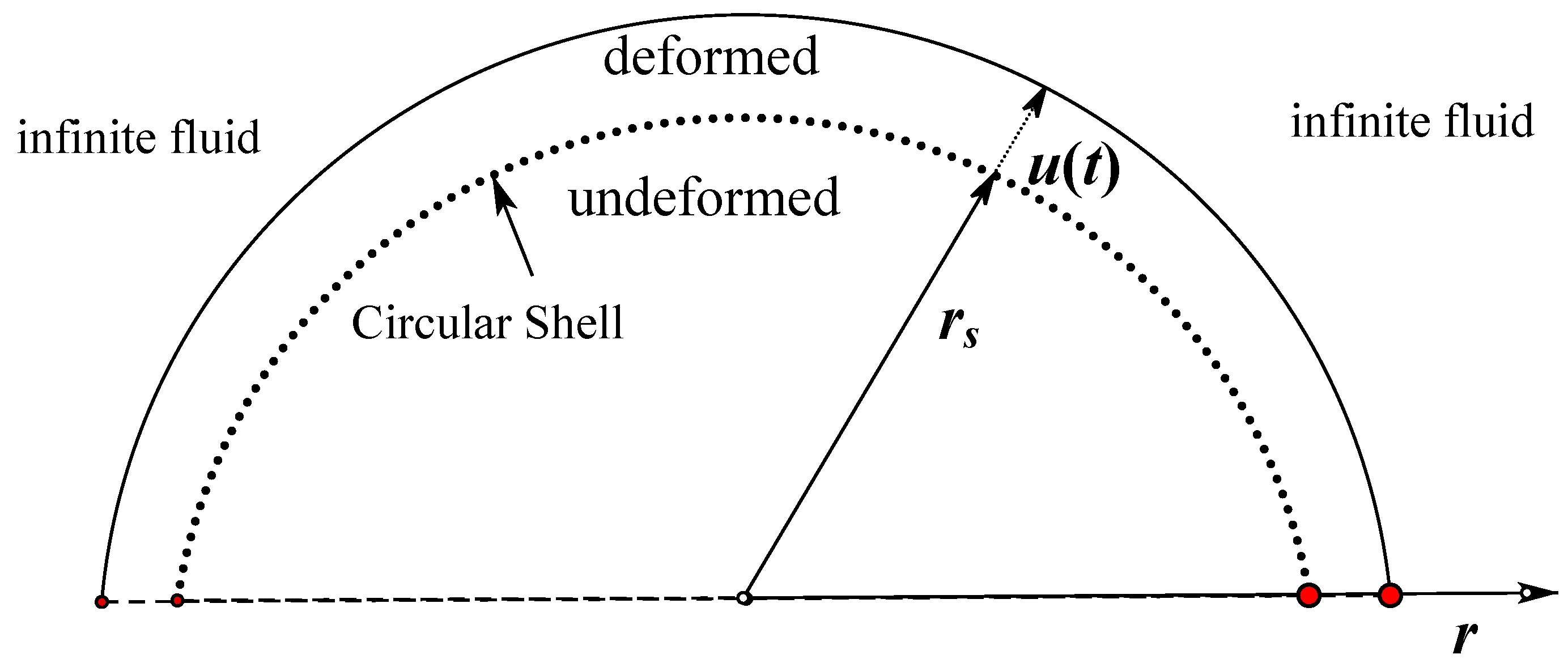
3.1. Case 1: A Cylindrical Shell

3.1.1. Model Details

The radius of the semi-circular shell is 10 m and the unbounded fluid was simulated as a far field boundary whose radius was 500 m (shown Figure 2a). The material properties of the fluid were set up as follows: Density = 1.225 kg/m³; sound velocity, c = 340 m/s. The viscosity is so small that it can be neglected in both the theoretical analysis and CFD calculation. The purpose of this paper is to investigate the principle of pressure under vibrations of a structure. The movement of a semi-circular shell was set as a uniform vibration in the radius direction. As for the calculation parameters, the far field boundary was set to be the far field pressure, the reference pressure value was zero, boundary movement (it is the same as the shell vibration) was set as U(t) = sin(10t), which is shown in Figure 2b, the calculating time was set to 1.0 s, and the delta-time to 0.001 s. A simple scheme second order method was accepted in the CFD simulation and the initial condition in fluid was set to a stationary condition. For comparison, two cases of a compressible and an incompressible fluid were carried out, respectively.

In order to present the effect of the discretization, numerical solutions with different meshing sizes are displayed.

Table 1. The total energy with different densities of mesh.

Density of Shell Mesh (cm)	2.0	1.0	0.8	0.5	0.3	0.2	0.1
Total energy (104 J)	4.52	4.21	3.93	3.90	3.89	3.88	3.88

shows the comparison of the total energy in the fluid, including kinetic energy and pressure potential energy, at t = 0.2 s. As the results in the case of a size of 0.2 m and 0.1 m are the same, the size of 0.2 m was thus adopted in this paper. Afterward, there were a total of 24,885 structural hexahedron elements in the numerical model.

3.1.2. Velocity Analyses

Figure 3 shows the relationship of the velocity vs. radius when t = 1.0 s. The continuous red line and green dot line show the value of the numerical result and the analytical solution in the case of the incompressible fluid and the compressible fluid, respectively. In the model described above, it is known that $s_r=0.294$, $J_1(s_r)=0.146$, $Y_1(s_r)=-2.334$, and $D=1$, therefore, the parameters can be derived as $C=0.425$, $\phi =-0.063$. For the case of the compressible fluid, the analytical solution is $u=-1.98\cos (10-r/34+2.3)/\sqrt{r}$, while for the case of the incompressible fluid, the analytical solution is $u=-5.44/r$. The correlation coefficients of the two figures are 0.982 and 0.937, respectively, which show that the analytical solutions and the numerical results are in good agreement. It can be concluded from the analytical solutions that the boundary motion is transmitted to the whole fluid instantly. Additionally, among the field of $r>ct$, all the fluid field remains in the initial situation. To show the whole shape of the analytical solution, the theoretical result was not cut off beyond the range of $r>ct$. That is why in Figure 3b, the data ranges from $r<350$ fits very well and some discrepancy exists between the numerical value and analytical solution in the range from $r>350$.

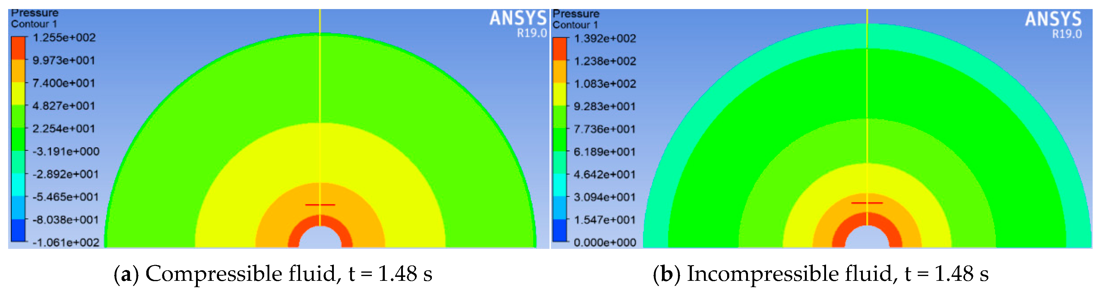
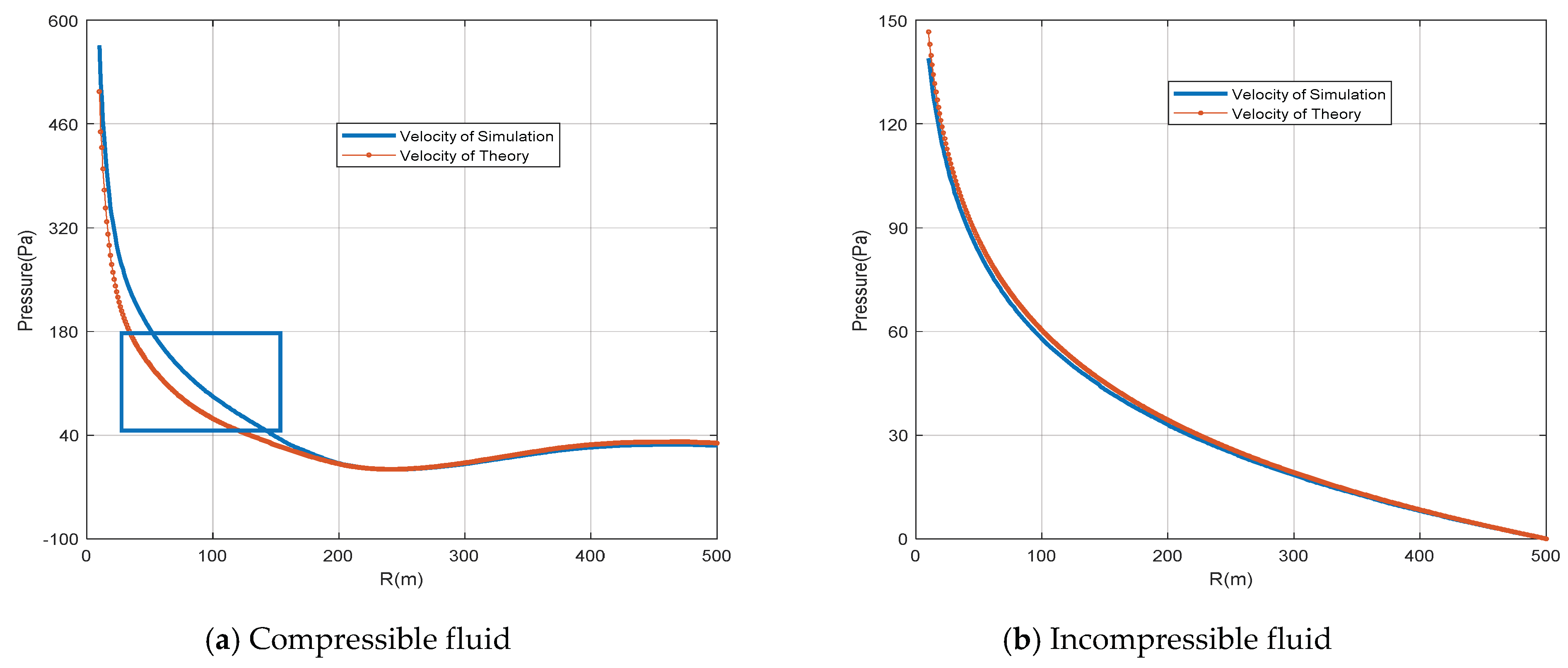
3.1.3. Pressure Analyses

Figure 4 shows the curve of pressure vs. radius at the condition of t = 1.0 s. The continuous line and dotted line of Figure 4a show the value of the numerical and theoretical result in the case of an incompressible fluid, while Figure 4b shows the result in the case of a compressible fluid. The correlation coefficients of the two figures are 0.973 and 0.928, respectively. It can be seen that the theoretical results fit the numerical results very well.

3.1.4. Pressure vs. Velocity

Figure 5 shows the relationship between the velocity and pressure under the assumption of a compressible fluid. The data of the blue circle expresses the numerical results and the red line expresses the linear line of the fitting curve via the least squares method. The results show that the numerical results are approximate to the linear relationship and the fitting coefficient is 418. The theoretical prediction is close to ${\rho }_{o}c$ = 417, which fits the result very well.

3.2. Case 2: Trigonal Velocity

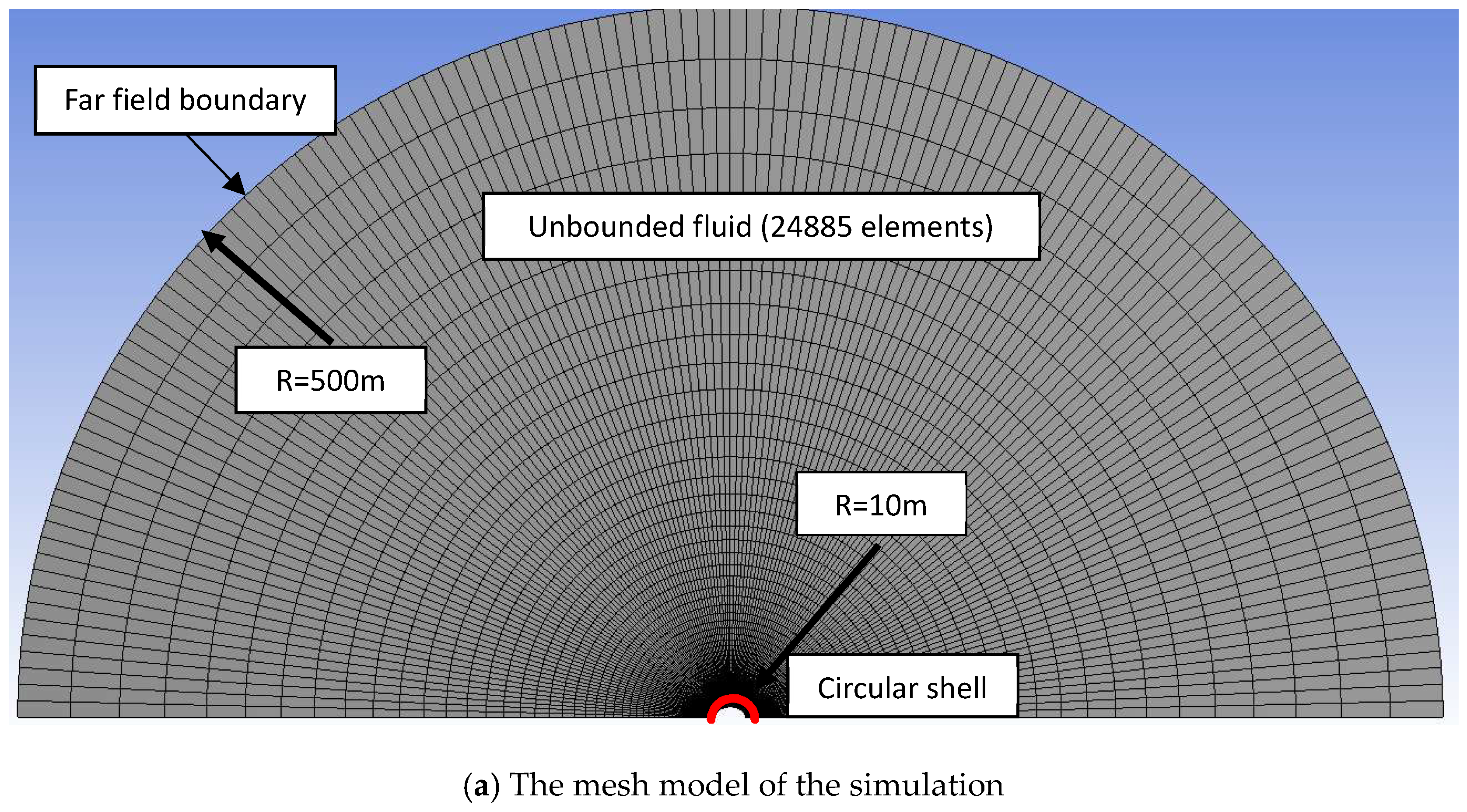
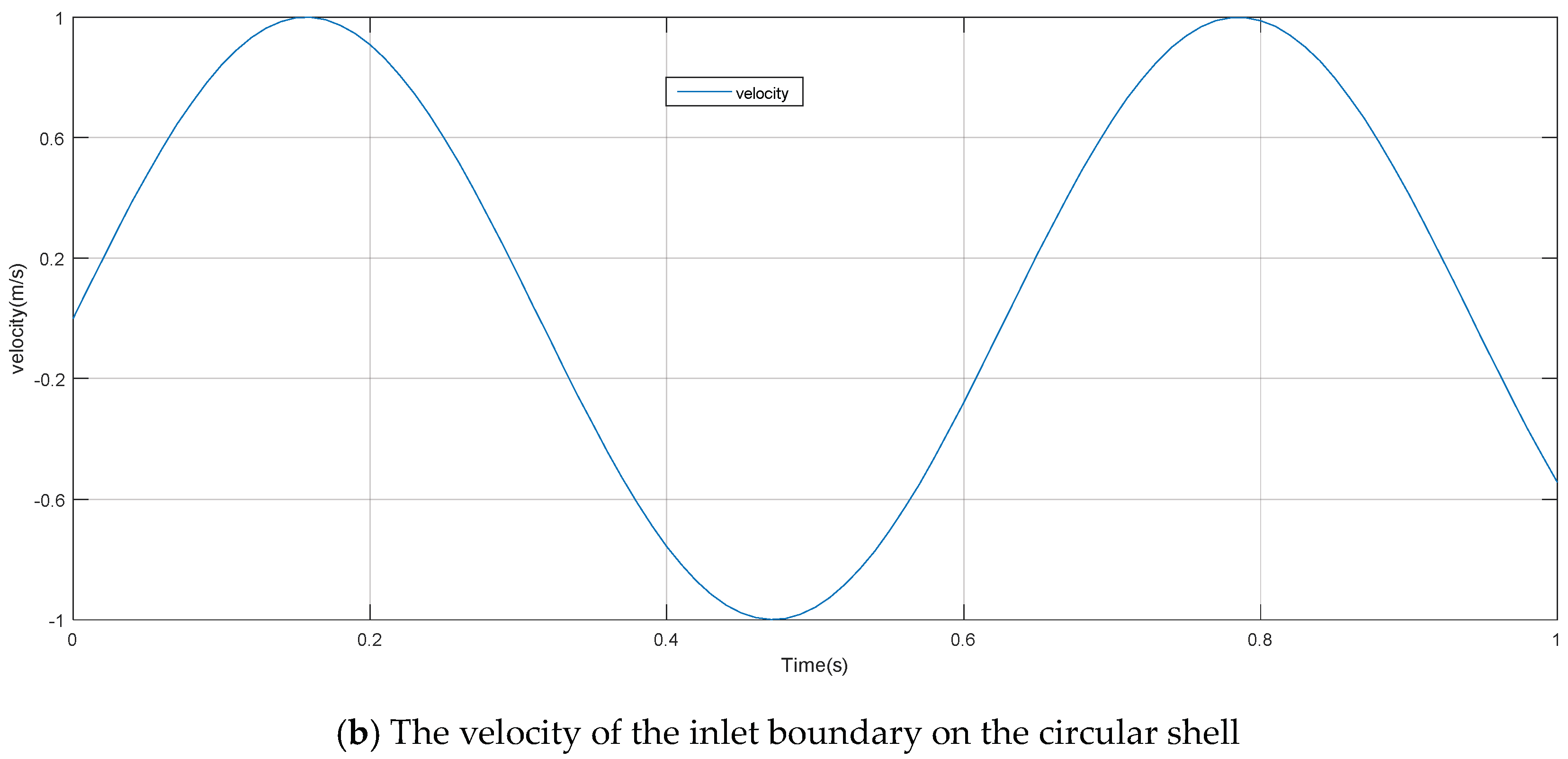
3.2.1. Simulation Model

To verify that this paper’s conclusion can be applied to the other velocity model, the simulation of trigonal velocity, which is written as Equation (34), was implemented, which is illustrated in Figure 6, and the other parameters were identical to case 1. In Equation (34), the function of round(t) returns a number rounded to a given digit:

$$v(t)=\{\begin{array}{l}3\cdot s,\\ 3-3\cdot s,\end{array},s=round(t)$$

(34)

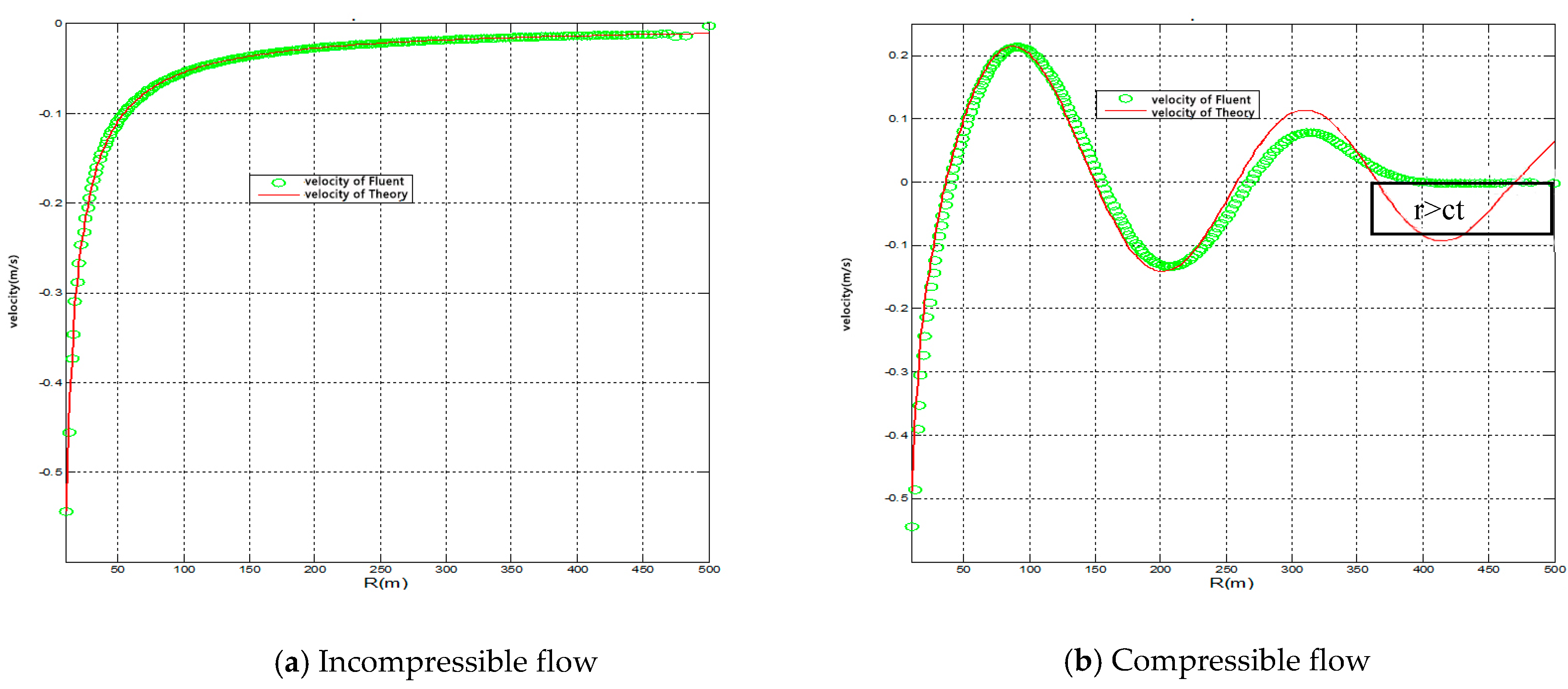
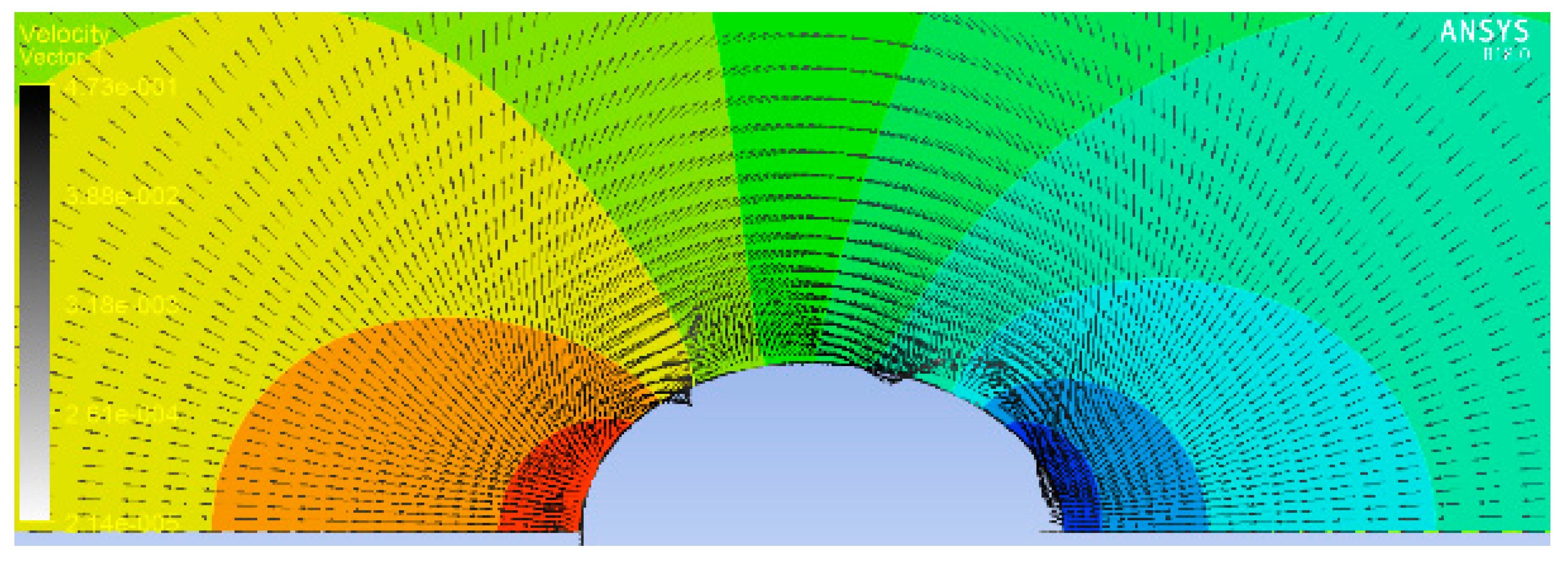
3.2.2. Velocity Analyses

As the velocity was a non-harmonica function, the velocity in case 2 could not be strictly evaluated by the conclusion above. In this section, Equation (21) is extended to be applied to the non-harmonica velocity. Figure 7a shows the velocity on the line [X = 0, Y = (10,500)], which is shown in Figure 8a. It presents that in the case of a compressible fluid, the result does fit not well, especially in the area marked by the blue rectangle, and there is a large discrepancy. However, in the case of an incompressible fluid, the result of the simulation fits with the theoretical result very well. This is because Equation (21) is based on the velocity being a harmonic function, which was described in Section 2.1. Additionally, it can be seen that there is no dominant frequency for the function of Equation (34) by the Fourier series, so the velocity of the inlet in case 2 does not agree with the harmonic function assumption, strictly. Figure 7b agrees with the theory very well as Equation (28) is true without the limitation of the harmonica function, which is described in Section 2.4.

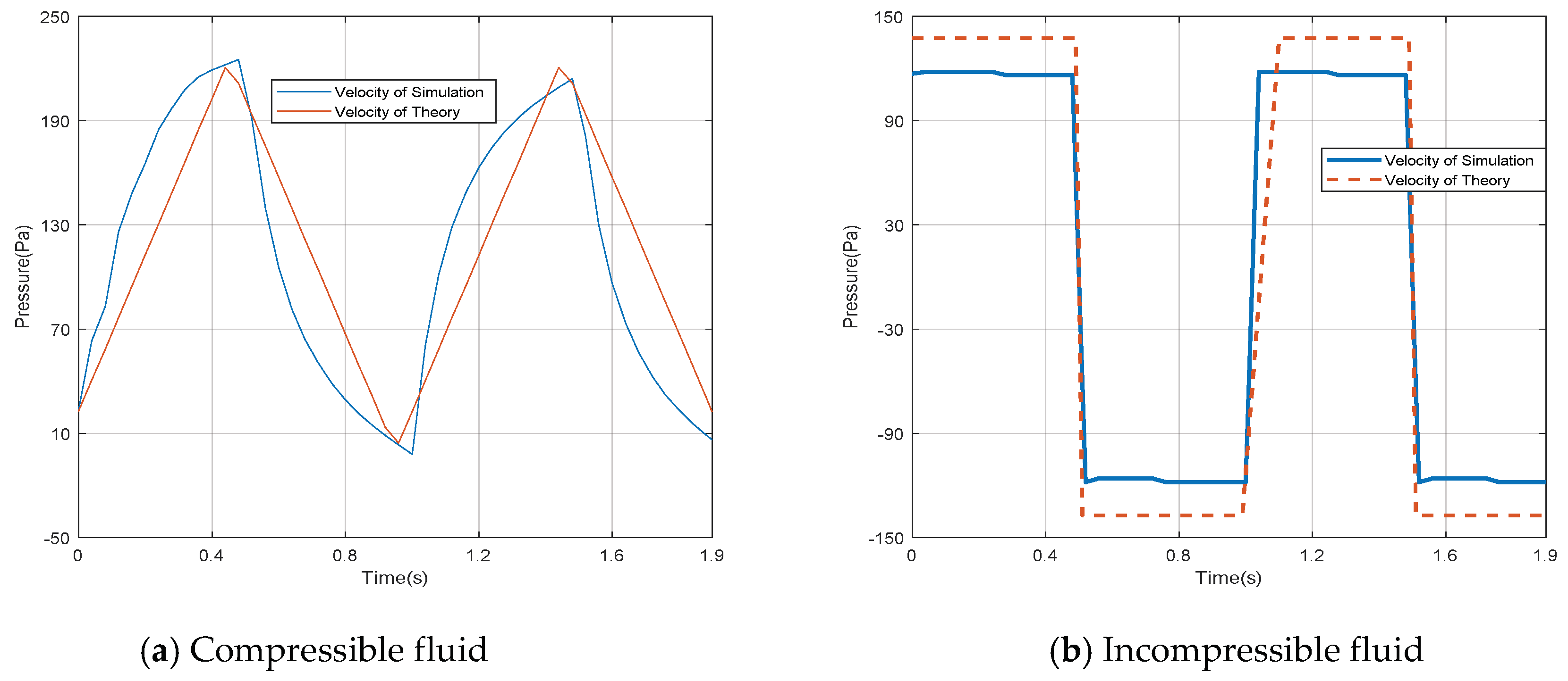
3.2.3. Pressure Analyses

In applications, the designer mostly cares more about pressure rather than the distribution of the velocity. Although the velocity is not the harmonica function, the pressure can be estimated by Equations (16) and (22). Figure 8 shows a contour map of the pressure when the time is 1.48 s.

Figure 9 illustrates the curve of pressure on the line of X = 0, Y = (10,500), which is shown in Figure 8. It is shown in Figure 9a that the result marked with the blue rectangle has some discrepancy compared with the other results that agree very well with the theory. Additionally, in the case of the incompressible fluid, the simulation results fit very well with the prediction of the theory.

3.2.4. Pressure vs. Velocity

As predicted in Equations (16) and (22), the pressure in the case of compressible fluid is proportional to the fluid velocity. The simulation and the theoretical result are shown in Figure 10a. There is some discrepancy nevertheless, but it can also be evaluated by the theoretical prediction. As for the incompressible fluid case, there is a very interesting result in that the pressure is the periodic step function, which the simulation agrees with very well. The error between the simulation and theory is about 17/143 = 12%, which may be caused by the numerical calculation and the simplification of the solution.

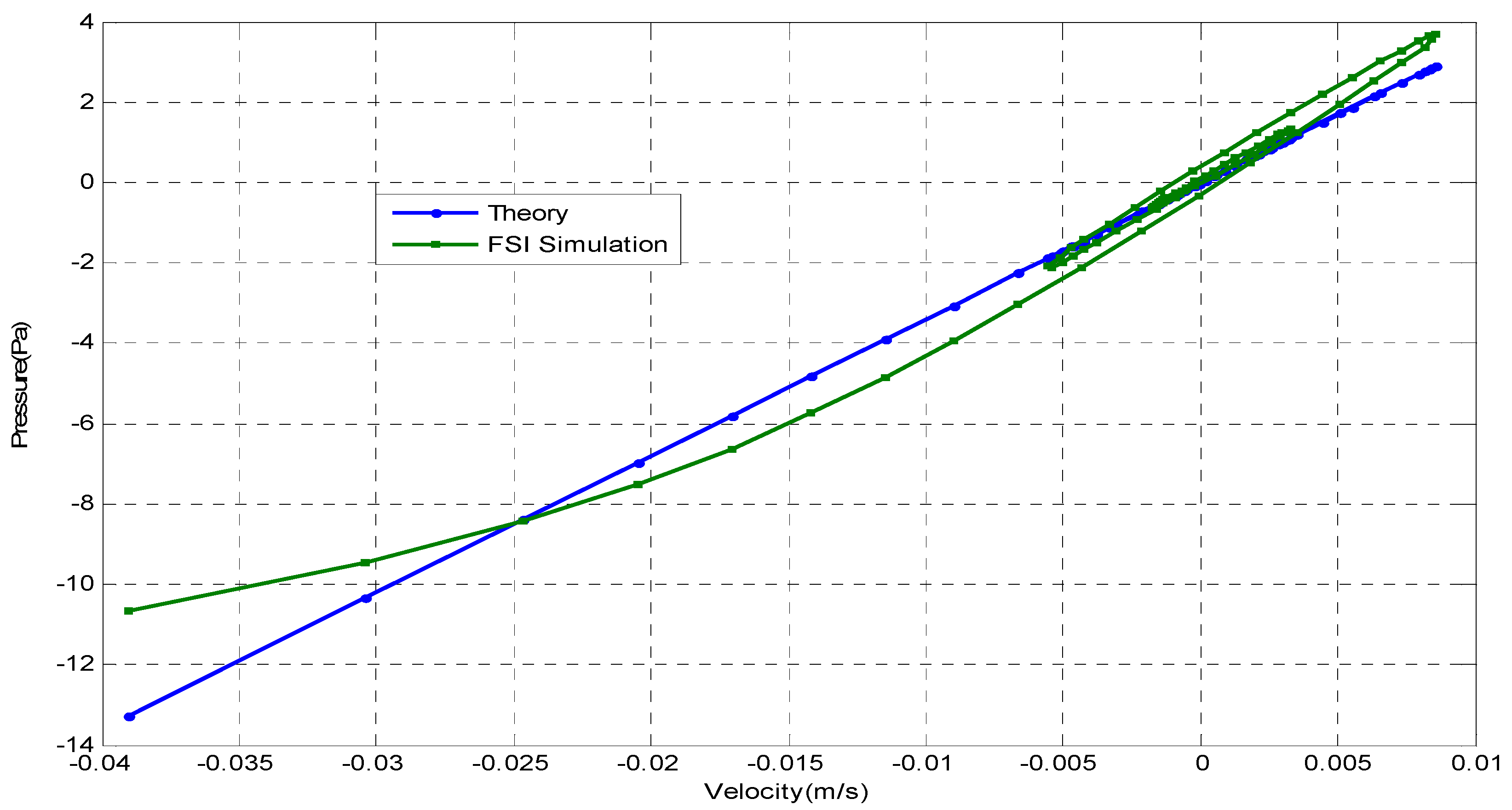
3.3 Case 3: FSI Model of the Elliptical Shell

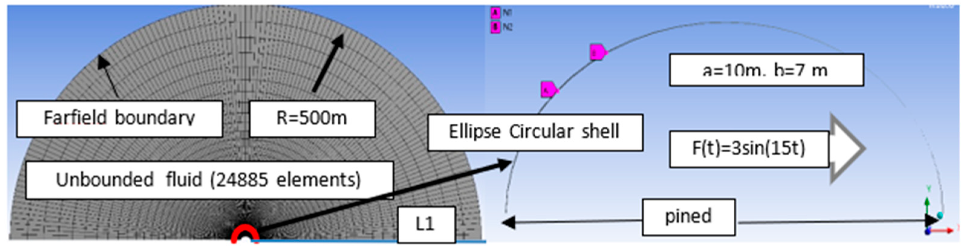
3.3.1. Model

An FSI simulation was completed to verify the validity of the theoretical conclusion via the module of the system coupling connecting the fluid solution and a transit solution. The simulation shown in Figure 11 was carried out by the loose coupled method. From the point of view of the fluid solution, all the parameters were identical to the model of case 1 except for the boundary, which was coupled to the structure analysis. From the point of view of the structure solution, the circular shell was set to an ellipse shape, and all the parameters are listed in

Table 2. Parameters of the FSI analysis.

Semi major axles (a)	10 m	Acceleration load	3 sin(15 t)	Yang’s module	210 GPa
Semi minor axles (b)	7 m	Boundary	pined	Poisson’s ratio	0.3
Thickness of shell	0.01 m	Total time	10 s	Delta time	0.01 s

. For comparison, the solo transit analysis via the theoretical pressure and Bernoulli method [41,42] were calculated. The results of point N1 and N2 marked in Figure 6 were discussed to verify the displacement result while the result on line L-1 was to verify the pressure solution.

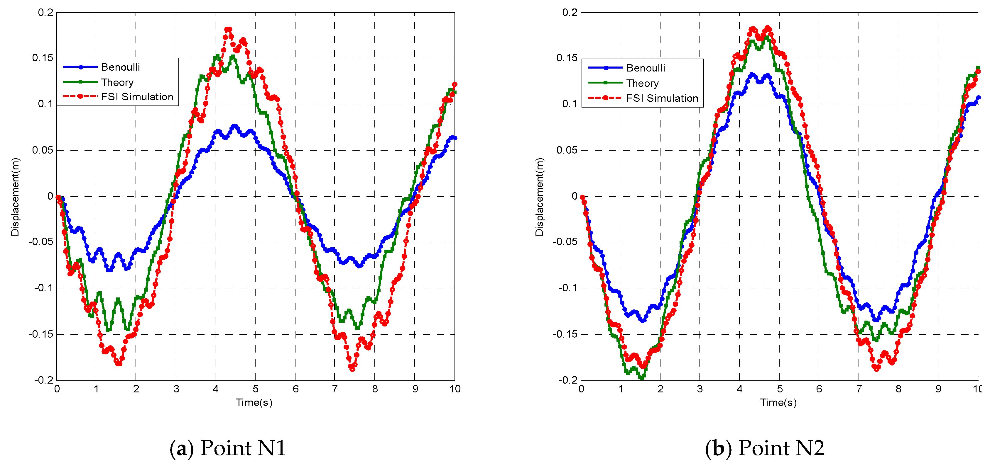
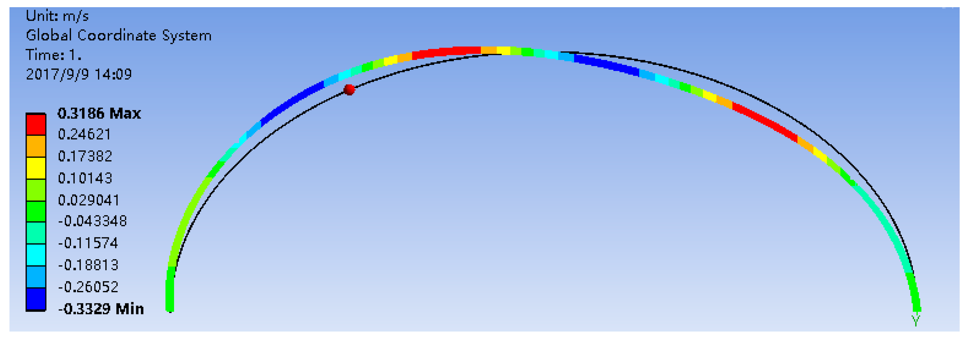
3.3.2. Displacement Results

Figure 12 presents the time history of the x-direction displacement in point N1 and point N2 of a circular shell vibrating under a sine wave load. Both plots show that the results calculated from theory are in good agreement with the results calculated from the FSI simulation. In contrast, the result from Bernoulli has a large gap from the FSI result.

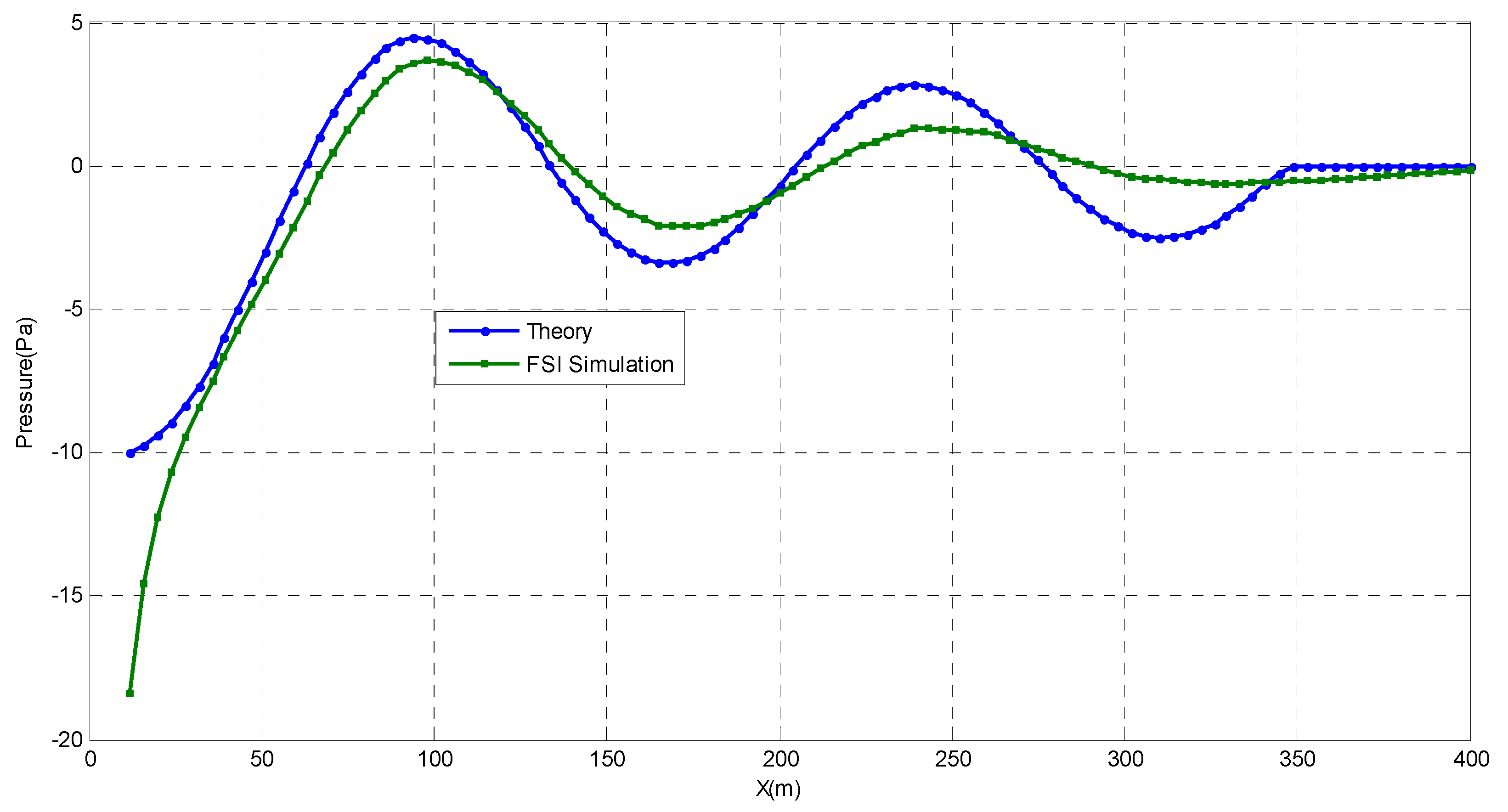
3.3.3. Pressure Results

Figure 13 shows the instantaneous pressure contour of fluid when t = 1.0 s and Figure 9 illustrates the velocity contour of a circular shell at the same time. According to Section 2 above, it is known that the circular shell is the boundary of the fluid; that is, the mean of the velocity of the boundary of the fluid is identical to the circular structure, which is verified by Figure 12 and Figure 13.

In addition, the streamline is shown in Figure 13. The streamlines generated from the boundary extend outside. It should be noticed that some part of the circular shell, seen as a red color in Figure 14, may vibrate back from the balance position, while some other part, seen as a blue color in Figure 14, may vibrate out from the balance position. The streamlines only come from the position of vibrating out to the position of vibrating back.

Figure 15 presents the relationship between the pressure on the line, L-1, and its x coordinate value. The theoretical results are in good agreement with the FSI simulation results. The plot of the pressure vs. velocity at the position, L-1, at t = 1.0 s is shown in Figure 16. The pressure is almost proportional to the velocity, which was predicted by the analytical solution.

4. Conclusions

Through the theoretical analysis of the vibration in the fluid of a circular shell structure, analytical solutions in both the incompressible fluid and compressible fluid were obtained. Compared with the numerical simulation results, the following conclusions can be made.

In the case of the incompressible fluid condition, the pressure of the structure is proportional to the boundary acceleration and it has a logarithmic relationship with the length of the flow field, which may result in unsolvable difficulties in the CFD solution. While under the condition of the compressible fluid, the boundary pressure is proportional to the velocity of the boundary and has nothing to do with the length of the flow field. Under the assumption of incompressible fluid, the effect of the pressure acting on the structure is equivalent to the added mass while in the case of compressible fluid, the pressure effect is equivalent to the viscous damping, and the damping ratio is ${\rho }_{o}c$, exactly. Under the incompressible fluid condition, the structural vibration is transmitted to the far field instantly while in the case of a compressible fluid, the vibration will be transmitted to the far field in a certain degree of time.

Via the new findings reported in this study, the dynamic pressure under the surface of a structure vibrated by an earthquake, boom blast, wind load, etc. can be accurately evaluated. The novel computational technique can also be applied to predict the effect of a fluid acting under the dynamic motion of a structure.

References

1. Liu, P.; Kaewunruen, S.; Zhou, D.; Wang, S.; Zhao, D.C.; Shang, S.W. Investigation of the Dynamic Buckling of Spherical Shell Structures Due to Subsea Collisions. Appl. Sci. 2018, 8, 1148. [Google Scholar] [CrossRef]
2. Liu, P.; Kaewunruen, S.; Tang, B. Dynamic Pressure Analysis of Hemispherical Shell Vibrating in Unbounded Compressible Fluid. Appl. Sci. 2018, 8, 1938. [Google Scholar] [CrossRef]
3. Zhang, J.; Zhang, M.; Cui, W.; Tang, W.; Wang, F.; Pan, B. Elastic-plastic buckling of deep sea spherical pressure hulls. Mar. Struct. 2018, 57, 38–51. [Google Scholar] [CrossRef]
4. Zhang, J.; Wang, M.; Cui, W.; Wang, F.; Hua, Z.; Tang, W. Effect of thickness on the buckling strength of egg- shaped pressure hulls. Ships Offshore Struct. 2018, 13, 375–384. [Google Scholar] [CrossRef]
5. Zhang, M.; Tang, W.; Wang, F.; Zhang, J.; Cui, W.; Chen, Y. Buckling of bi-segment spherical shells under hydrostatic external pressure. Thin-Walled Struct. 2017, 120, 1–8. [Google Scholar] [CrossRef]
6. Chakrabarti, K.; Frampton, R.E. Review of riser analysis techniques. Appl. Ocean Res. 1982, 4, 80–90. [Google Scholar] [CrossRef]
7. Pang, S.; Gao, Y.; Choi, S. Flexible and stretchable microbial fuel cells with modified conductive and hydrophilic textile. Biosens. Bioelectron. 2018, 100, 504–511. [Google Scholar] [CrossRef]
8. Zhou, X.; Gosling, P.D. Influence of stochastic variations in manufacturing defects on the mechanical performance of textile composites. Compos. Struct. 2018, 194, 226–239. [Google Scholar] [CrossRef]
9. Kariou, F.A.; Triantafyllou, S.P.; Bournas, D.A.; Koutas, L.N. Out-of-plane response of masonry walls strengthened using textile-mortar system. Constr. Build. Mater. 2018, 165, 769–781. [Google Scholar] [CrossRef]
10. Da Silva Monteiro, L.L.; Netto, T.A.; Da Camara Monteiro, P.C., Jr. On the Dynamic Collapse of Cylindrical Shells Under Impulsive Pressure Loadings. J. Offshore Mech. Arct. 2016, 138, 041101. [Google Scholar] [CrossRef]
11. Wu, X.; Ge, F.; Hong, Y. A review of recent studies on vortex-induced vibrations of long slender cylinders. J. Fluid Struct. 2012, 28, 292–308. [Google Scholar] [CrossRef]
12. Trivedi, C. A review on fluid structure interaction in hydraulic turbines: A focus on hydrodynamic damping. J. Fluid Dyn. 2016, 35, 333–349. [Google Scholar] [CrossRef]
13. Suarez, L.E.; Gaviria, C.A. Equivalent Frequencies and Damping Ratios of Buildings with Viscous Fluid Dampers: A Closed Form Formulation; Earthquake Engineering Research Institute: Anchorage, AK, USA, 2014. [Google Scholar]
14. Mattioli, M.; Mancinelli, A.; Brocchini, M. Experimental investigation of the wave-induced flow around a surface-touching cylinder. J. Fluid Struct. 2013, 37, 62–87. [Google Scholar] [CrossRef]
15. Minami, H. Added mass of a membrane vibrating at finite amplitude. J. Fluid Struct. 1998, 12, 919–932. [Google Scholar] [CrossRef]
16. Kubenko, V.D.; Dzyuba, V.V. Resonance phenomena in cylindrical shell with a spherical inclusion in the presence of an internal compressible liquid and an external elastic medium. J. Fluid Struct. 2006, 22, 577–594. [Google Scholar] [CrossRef]
17. Sorokin, S.V.; Terentiev, A.V. Flow-induced vibrations of an elastic cylindrical shell conveying a compressible fluid. J. Sound Vib. 2006, 296, 777–796. [Google Scholar] [CrossRef]
18. Chung, M.H. Hydrodynamics of flow over a transversely oscillating circular cylinder beneath a free surface. J. Fluid Struct. 2015, 54, 27–73. [Google Scholar] [CrossRef]
19. Calautit, J.K.; O’Connor, D.; Hughes, B.R. Determining the optimum spacing and arrangement for commercial wind towers for ventilation performance. Build. Environ. 2014, 82, 274–287. [Google Scholar] [CrossRef] [Green Version]
20. Liberge, E.; Hamdouni, A. Reduced order modelling method via proper orthogonal decomposition (POD) for flow around an oscillating cylinder. J. Fluid Struct. 2010, 26, 292–311. [Google Scholar] [CrossRef]
21. Munch, C.; Ausoni, P.; Braun, O.; Farhat, M.; Avellan, F. Fluid-structure coupling for an oscillating hydrofoil. J. Fluid Struct. 2010, 26, 1018–1033. [Google Scholar] [CrossRef]
22. Rojratsirikul, P.; Wang, Z.; Gursul, I. Effect of pre-strain and excess length on unsteady fluid-structure interactions of membrane airfoils. J. Fluid Struct. 2010, 26, 359–376. [Google Scholar] [CrossRef]
23. Karagiozis, K.; Kamakoti, R.; Cirak, F.; Pantano, C. A computational study of supersonic disk-gap-band parachutes using Large-Eddy Simulation coupled to a structural membrane. J. Fluid Struct. 2011, 27, 175–192. [Google Scholar] [CrossRef]
24. Al-Gahtani, H.; Khathlan, A.; Sunar, M.; Naffaa, M. Local Hydrostatic Pressure Test for Cylindrical Vessels. J. Press. Vess.-Technol. ASME 2017, 139, 011601. [Google Scholar] [CrossRef]
25. Li, T.Y.; Wang, P.; Zhu, X.; Yang, J.; Ye, W.B. Prediction of Far-Field Sound Pressure of a Semi-submerged Cylindrical Shell with Low-Frequency Excitation. J. Vib Acoust. 2017, 139, 041002. [Google Scholar] [CrossRef]
26. Lawrence, V.; Ngamkhanong, C.; Kaewunruen, S. An Investigation to Optimize the Layout of Protective Blast Barriers Using Finite Element Modelling. Mater. Sci. Eng. 2017, 280, 375–383. [Google Scholar] [CrossRef]
27. Saadin, B.; Leena, S.; Sakdirat, K.; David, J. Operational Readiness for Climate Change of Malaysia High-Speed Rail; University of Birmingham: Birmingham, UK, 2016. [Google Scholar]
28. Kaewunruen, S. Underpinning systems thinking in railway engineering education. Australas. J. Eng. Educ. 2017, 22, 107–114. [Google Scholar] [CrossRef]
29. Cholcz, T.P.S.; van Zuijlen, A.H.; Bijl, H. Space-mapping in fluid-structure interaction problems. Comput. Method Appl. Mech. Eng. 2014, 281, 162–183. [Google Scholar] [CrossRef]
30. Motiei, P.; Yaghoubi, M.; GoshtashbiRad, E.; Vadiee, A. Two-dimensional unsteady state performance analysis of a hybrid photovoltaic-thermoelectric generator. Renew. Energ. 2018, 2018, 551–565. [Google Scholar] [CrossRef]
31. Naccache, G.; Paraschivoiu, M. Parametric study of the dual vertical axis wind turbine using CFD. J. Wind Eng. Ind. Aerodyn. 2018, 2018, 244–255. [Google Scholar] [CrossRef]
32. Wua, G.; Qin, Z.; Zhang, L.; Yang, K. Strain response analysis of adhesively bonded extended composite wind turbine blade suffering unsteady aerodynamic loads. Eng. Fail Anal. 2018, 2018, 36–49. [Google Scholar] [CrossRef]
33. Wang, S.; Chen, Y.; Liu, Y.Z. Measurement of unsteady flow structures in a low speed wind tunnel using continuous wave laser-based TR-PIV: Near wake behind a circular cylinder. J. Visous 2018, 2018, 73–93. [Google Scholar] [CrossRef]
34. Tang, J.; Hu, Y.; Song, B.; Yang, H. An unsteady free wake model for aerodynamic performance of cycloidal propellers. J. Aerosp. Eng. 2018, 223, 290–307. [Google Scholar] [CrossRef]
35. Jiang, L.; Li, J.; Li, C. Comparative Study on Non-Gaussian Characteristics of Wind Pressure for Rigid and Flexible Structures. Shock Vib. 2018, 2018, 1–26. [Google Scholar] [CrossRef] [Green Version]
36. Basnet, K.; Constantinescu, G. The structure of turbulent flow around vertical plates containing holes and attached to a channel bed. Phys. Fluids 2017, 2017, 1147–1156. [Google Scholar] [CrossRef]
37. Li, Q.; Maeda, T.; Kamada, Y.; Hiromori, Y.; Nakai, A.; Kasuya, T. Study on stall behavior of a straight-bladed vertical axis wind turbine with numerical and experimental investigations. J. Wind Eng. Ind. Aerod. 2017, 164, 1–12. [Google Scholar] [CrossRef]
38. Mattheij, R.M.M.; Rienstra, S.W.; Boonkkamp, J.H.M.T. Partial Differential Equations: Modeling, Analysis, Computation; Siam: Philadelphia, PA, USA, 2005. [Google Scholar]
39. Evans, L.C. Partial Differential Equations, 1st ed.; American Mathematical Society: Providence, RI, USA, 1998. [Google Scholar]
40. Ya, L.; Hong, Y.J. The interaction between membrane structure and wind based on the discontinuous boundary element. Sci. China Technol. Sci. 2010, 53, 486–501. [Google Scholar]
41. Si, X.H.; Lu, W.X.; Chu, F.L. Modal analysis of circular plates with radial side cracks and in contact with water on one side based on the Rayleigh–Ritz method. J. Sound Vib. 2012, 331, 231–251. [Google Scholar] [CrossRef]
42. Kaewunruen, S.; Sussman, J.M.; Matsumoto, A. Grand challenges in transportation and transit systems. Front. Built Environ. 2016, 2, 4. [Google Scholar] [CrossRef]
Figure 1. The schematic states of the vibration of the cylindrical shell.
Applsci 09 01403 g001
Figure 2. The circular symmetry model of a semi-circular shell vibrating in unbounded velocity.
Applsci 09 01403 g002aApplsci 09 01403 g002b
Figure 3. Validation of the velocity vs. radius when t = 1.0 s.
Applsci 09 01403 g003
Figure 4. Validation of pressure vs. radius when t = 1.0 s.
Applsci 09 01403 g004
Figure 5. The relationship of velocity and pressure in compressible fluid.
Applsci 09 01403 g005
Figure 6. The velocity of the trigonal case.
Applsci 09 01403 g006
Figure 7. The plot of the velocity on the line X = 0, Y = (10,500) in case 2.
Applsci 09 01403 g007
Figure 8. The plot of the pressure of case 2 with compressible fluid and incompressible fluid.
Applsci 09 01403 g008
Figure 9. The pressure of case 2 on the line X = 0, Y = (10,500).
Applsci 09 01403 g009
Figure 10. The pressure of case 2 on the line X = 0.
Applsci 09 01403 g010
Figure 11. Schematic diagram of the FSI mode.
Applsci 09 01403 g011
Figure 12. The time history of the X-direction displacement at the point of N1 and N2.
Applsci 09 01403 g012
Figure 13. The instantaneous contours of velocity when t = 1.0 s.
Applsci 09 01403 g013
Figure 14. The velocity response in the y-direction of the circular shell when t = 1.0 s.
Applsci 09 01403 g014
Figure 15. Pressure at the position, L-1, when t = 1.0 s.
Applsci 09 01403 g015
Figure 16. The relationship of pressure vs. velocity.
Applsci 09 01403 g016