Abstract
At present, digital maps can estimate the travel time of each trip’s route but cannot offer a fuel consumption estimation at the same time. In this paper, we develop a fuel consumption model based on the Vehicle Specific Power (VSP) distribution, which can connect the traffic condition prediction with the fuel consumption model to predict fuel consumption. First, the traffic condition forecasting and the trip time of each route can be obtained through the digital map Application Programming Interface (API). Secondly, the users need to provide the engine displacement of their vehicles to match the fuel consumption model. Then, the fuel consumption prediction application based on Android is developed to forecast the fuel consumption by using traffic prediction data. Finally, the fuel consumption provided by the On-Board Diagnostic (OBD) data is used to verify the proposed application, and the forecasting error is less than 20%.
1. Introduction
With the development of digital maps and mobile internet, drivers rely increasingly on route guidance services, which can tell drivers the predicted trip time of each route. However, currently, there is no fuel consumption prediction to help drivers select the most fuel-efficient route. The aim of this study is to develop a fuel consumption prediction model by combining digital maps with traditional fuel consumption models.
The traditional fuel consumption models can be divided into two types: statistical fuel consumption models and theoretical fuel consumption models. The statistical fuel consumption model focuses on the statistical properties of fuel consumption data and vehicle activity data (speed and acceleration), whereas the theoretical fuel consumption model pays more attention to the characteristics of the vehicle’s operation, such as the engine parameters and vehicle output power [1,2,3]. The theoretical model requires complex and difficult model input which has closed physical relationships with the vehicle fuel consumption. Therefore, the theoretical model shows higher accuracy and lower applicability. According to the parameters which are used in fuel consumption models, the model can be classified as a fuel consumption model based on speed-acceleration statistics [4], a fuel consumption model based on operating mode decomposition [5,6] or a power demand model [7,8,9]. In general, the statistical model based on speed-acceleration is the most simple and intuitive, but the disadvantage is that it does not differentiate the vehicle operating mode, which leads to a larger error in the fuel consumption calculation. The operating mode decomposition model has a satisfactory result in calculating the fuel consumption of a long trip, but it has poor performance in gaining accurate fuel consumption for a short trip whose distance is shorter than 4 km [10]. In recent years, a power demand parameter, Vehicle Specific Power (VSP), based on vehicle speed and acceleration, has been developed and can be used to describe the power of the vehicle during the actual driving process. It has a strong correlation with the vehicle fuel consumption and emissions [11]. The distribution of VSP can better reflect the different vehicle operating modes; thus, this model based on power demand is widely used [12,13,14].
On the other hand, the traditional fuel consumption model is used to calculate the fuel consumption when the trip data are already known [15,16]; it cannot forecast the fuel consumption before the trip. Xiang et al. [17] took the trip time and intersection distance as research parameters, constructing a macroscopic model of fuel consumption and provide a basic prediction method.
Most the smartphone research on transportation is based on the diversity and breadth of the smartphone data. This includes some calculation of instantaneous fuel consumption [18], keeping the equilibrium of road traffic flow by using the information shared by smartphone [19] and testing the accuracy of the certified fuel consumption level [20].
In this paper, the traffic condition prediction and fuel consumption models are important elements of realizing fuel consumption prediction. Furthermore, the VSP distribution is the key to connecting these two elements. The final representation form is a smartphone application.
2. Data Collection and Processing
2.1. Data Source
In this paper, the On-Board Diagnostic (OBD) collector we used is Y-BOX300, as shown in Figure 1. It is plugged into the tested vehicles’ OBD socket to collect vehicle trip data and trajectory data. The trip data include the average speed, distance, time, and fuel consumption of each trip, and the location data, i.e., the trip origin and destination. The vehicle trajectory data involves second-by-second fuel consumption data, instantaneous speed data and GPS data. The two types of data are shown in Table 1 and Table 2.
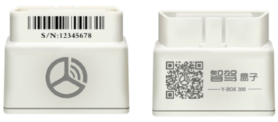
Figure 1.
The Y-BOX300.

Table 1.
The sample of the trajectory data.
Table 3 indicates the time, location and size of data.
Table 3.
The general information about the data.
Among these, each of the 143 vehicles has more than one trip record. In this study, all the tested vehicles are light-duty vehicles in Beijing; we only used gasoline vehicles because light-duty diesel vehicles are forbidden in Beijing.
2.2. Data Quality Control
The following data process is applied to clean the abnormal data:
- Eliminating the data with a fuel consumption greater than 100 mL per second according to the fuel consumption information of track data because the proportion of data on vehicles whose fuel consumption is more than 100 mL per second is less than 0.1%.
- Eliminating the data with a speed greater than 40 m per second based on the distance stamp information of the track data because the proportion of data on vehicles whose speed is more than 40 m per second is less than 0.1%.
3. Methodology
3.1. Division Speed Interval
The fuel consumption prediction model is based on the traffic condition predictions of the digital map. Given that the digital map can only predict a vehicle’s operating mode over a time span, not on a second-by-second basis, all the vehicle trajectory data and fuel consumption data will be divided into many segments, which contain 60 s of continuous data. Then the average speed of each segment can be calculated by Equation (1).
where is the average trip speed in the unit of , is the trip distance in the unit of , is the driving time in the unit of , and is the speed of the i-th second in the unit of .
The traffic condition prediction is captured through the Application Programming Interface (API) of a digital map, which divides the traffic conditions into four types. Hence, the data segments are divided into four groups to match the traffic condition predictions according to the average speed of each segment. Table 4 shows the correspondences.
Table 4.
The correspondences between the speed interval and traffic conditions prediction.
3.2. Calculation of VSP and Determination of VSP Bin
Created by Song and Yu [21], the formula for calculating the VSP in urban roads appears in Equation (2). In this formula, we do not consider the gradient of the slope on the road because the data collection was done in Beijing in the North China Plain:
where is the vehicle specific power in the unit of , v is the instantaneous speed in the unit of m/s, and a is the acceleration in the unit of .
Based on the equation, the instantaneous speed v and the instantaneous acceleration a are used to calculate the instantaneous VSP; v and a can be obtained from the vehicle trajectory data.
To analyze the relationship between VSP and fuel consumption, cluster analysis is applied in VSP, by dividing VSP into several intervals called VSP bin. The time ratio of a vehicle under each VSP bin within a certain time is called VSP distribution.
The existing research of VSP puts forward a variety of VSP interval partition methods to simplify the computation [22,23]. In this study, VSP distribution can be obtained (Figure 2) after the calculations of VSP are implemented in Equation (2). Previous studies [20,21] showed that the distribution of VSP value is concentrated at –2019 . To avoid any bias being incorporated into the VSP binning, an interval of 1 kW/ton is used. The binning method is written in Equation (3):
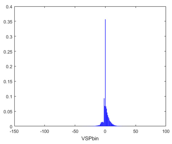
Figure 2.
The Vehicle Specific Power (VSP) distribution.
3.3. VSP Distribution at Different Speed Intervals
According to Song and Yu’s research [21], when the average trip speed is larger than 20 km/h, the distribution of the VSP fits well with the normal distribution. The probability density function is
where is the mean of distribution and is the standard deviation of the distribution. Both and can be calculated according to the average speed in each speed interval.
The trajectory data in different speed intervals are used to calculate the VSP distribution and the results are shown in Figure 3.
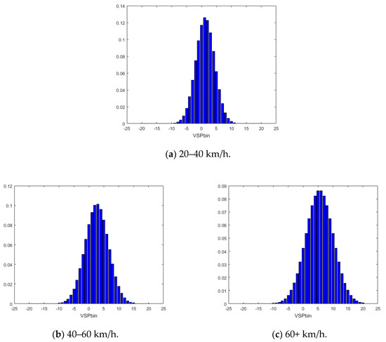
Figure 3.
The Vehicle Specific Power distribution at different speed intervals.
When the average trip speed is less than 20 km/h, the ratio of VSP = 0 is larger than that of other regions, which does not conform to the normal distribution. Thus, according to historical On-Board Diagnostic (OBD) data, we obtained the distribution shown in Figure 4.
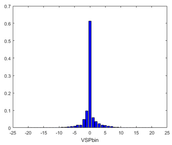
Figure 4.
The Vehicle Specific Power distribution in the speed interval under 20 km/h.
3.4. The Model of VSP-Fuel Consumption in Different Speed Intervals
It was proven that VSP has a strong correlation with fuel consumption. Figure 5 presents a scatter diagram of VSP-fuel consumption rate and it can be seen that there is an obvious change trend when VSP equals 0. Thus, the unified regression model of all VSP data cannot well reflect the relationship between VSP and fuel consumption. In this paper, the data in different speed intervals are divided into two parts according to VSP (greater than zero or less than zero), and the VSP and fuel consumption rate are analyzed by regression analysis. In addition, to reduce the scatter of fuel consumption rate in each VSP bin, the average fuel consumption rate corresponding to each VSP bin is calculated. Because the data processing methods in these two conditions (VSP > 0 and VSP < 0) are the same, only the regression analysis results when VSP > 0 are shown in Figure 6. Further, the correlation coefficients are above 0.9.
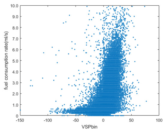
Figure 5.
The VSP-fuel consumption scatter plot.
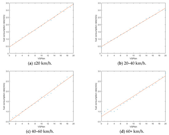
Figure 6.
The regression results after the cluster analysis of the VSP bin.
For Figure 6, linear regression was a good method to solve the consumption model. The fuel consumption model is described concretely from Equation (7):
is the fuel consumption rate in different VSP regions, and and are the regression coefficients. It is known that the fuel consumption rates of different vehicle types are significantly different, even under the same traffic conditions and operating mode. Many factors, such as the vehicle weight, engine displacement, and model year, affect the level of fuel consumption. Considering the limitations of the OBD data dimension in this paper, engine displacement is applied to differentiate the vehicle types. Then the OBD data are divided according to the interval of engine displacement in Table 5.
Table 5.
The intervals of engine displacement.
If the vehicle has turbocharged engines, it would be put in the higher interval. For example, the vehicle with a 2.0-L turbocharged engine will belong to interval 3.
After data partitioning, the coefficient and of Equation (7) can be obtained through the calculation of different engine displacement intervals and different speed intervals, as shown in Table 6.
Table 6.
The model parameters.
3.5. Fuel Consumption Rate in Different Speed Intervals and Engine Displacement Intervals
After the construction of VSP distribution and fuel consumption model at different speed intervals, the fuel consumption rate in each speed interval is calculated according to Equation (8).
where is the rate of fuel consumption in the speed interval of k in the unit of mL/s, is the rate of fuel consumption in the VSP interval of in the unit of mL/s, and is the distribution of i-th VSP interval in the kth speed interval.
After calculation, the fuel consumption rates in each speed interval and engine displacement intervals are recorded, as shown in Table 7.
Table 7.
The fuel consumption rates in each speed interval and engine displacement interval.
4. Development and Verification of Application
4.1. Fuel Consumption Prediction Application Interface and Functions
In order to realize the fuel consumption model proposed above, a smartphone application based on Android was developed. The application is used to gain specific trip information and offer the fuel consumption prediction of each route.
The users need to enter the details of their engine displacement, and the origin and destination, then the trip time in different speed intervals of each route can be obtained through the API of the Baidu Map (a digital map in China), and the fuel consumption prediction can be served by the proposed model. The flow chart of the fuel consumption prediction is shown in Figure 7. It includes three parts, the mobile phone program, the server and the network communication between them. Mobile phone programs are used to interact with users, such as by obtaining the trip paths selected by users and displaying the fuel consumption prediction. The server is used to calculate fuel consumption. The transmission contents between mobile phones and the server are trip paths selected by users and the fuel consumption prediction. Figure 8 shows the interface of the application: the selection of the origin and destination, the selection of trip paths, and the corresponding fuel consumption prediction.
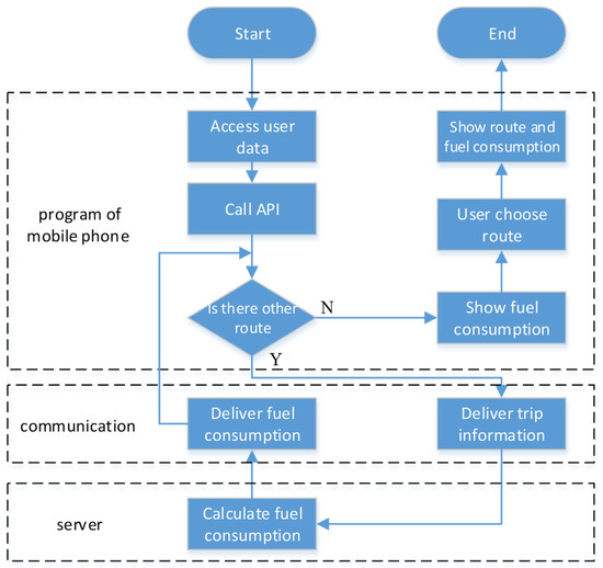
Figure 7.
The specific flow chart of the fuel consumption predictions.
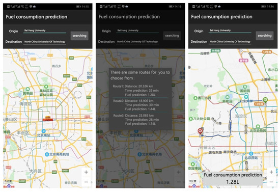
Figure 8.
The application interface.
4.2. Error Analysis
According to some existing research, the difference between the fuel consumption data calculated from the OBD data and the measured fuel consumption data is acceptable [24,25]. Thus, in order to verify the accuracy of the model, three trips are selected randomly in each interval of engine displacement from OBD data. There is a total of 12 trips’ fuel consumption data used to verify the proposed application. Table 8 shows the results.
Overall, it can be seen that the average error of the VSP distributed fuel consumption model can be controlled at 20%. The trips with an error higher than 15% are analyzed concretely and results are shown in Table 9. It can be seen that the time proportion of the low-speed intervals is large on these trips. Considering the irregularity of the VSP distribution in the low-speed interval, it is difficult to distinguish the idle state from the low-speed driving state in the prediction, which leads to a large error.
Table 9.
The comparison of time proportion.
5. Conclusions
According to error analysis, the error of fuel consumption prediction is high when the time proportion of the low-speed interval is large. This phenomenon proves the irregular form of the VSP distribution when the average trip speed is lower than 20 km/h. Overall, the error of the proposed model is less than 20%.
As a fuel consumption prediction model, an error of 20% is larger than that in the traditional fuel consumption model. However, it can match all kinds of vehicle operating modes defined by the digital map because the input of the model is only the driving time of each speed interval. According to the time information provided by the digital map, the fuel consumption can be predicted.
The model year of the vehicle also has a great influence on fuel consumption, which is not taken into account in the proposed model. In future research, the data dimension can be enriched and the parameter and year of the vehicle can be used as correction factors to improve the accuracy of the fuel consumption prediction. Additionally, in the field of automotive engineering, there is a significant difference in the running mechanism of the engine between cold and hot starts so that the impact on the fuel consumption is also worth paying attention to. In addition, the OBD data is treated as real in the error analysis although some research has proven that the difference between the fuel consumption data calculated from the OBD data and the measured fuel consumption data is acceptable. Nonetheless, it is still the main limitation of this research. Therefore, if the data sources are more abundant in the future, the error of the fuel consumption prediction model can be further explored. The real fuel consumption could also be used as the correction factor to improve the prediction accuracy.
Author Contributions
In this study, the research idea and methodology are put forward by Q.Z., data curation and manuscript editing are accomplished by Q.C., and L.W. was responsible for manuscript review.
Funding
This research was supported by grants from the North China University of Technology Startup Fund and the Great Wall Scholar Program (CIT&TCD20190304).
Acknowledgments
The authors acknowledge the supports of this paper by Beijing Jiaotong University and also thank the employees of Zhijia Travel Technology Co., Ltd. for providing the OBD data used in this study.
Conflicts of Interest
The authors declare there is no conflict of interest regarding the publication of this paper.
References
- Silva, C.M.; Gonçalves, G.A.; Farias, T.L.; Mendes-Lopes, J.M.C. A tank-to-wheel analysis tool for energy and emissions studies in road vehicles. Sci. Total Environ. 2006, 367, 441. [Google Scholar] [CrossRef] [PubMed]
- Barth, M. The Comprehensive Modal Emission Model (CMEM) for Predicting Light-Duty Vehicle Emissions. In Transportation Planning and Air Quality IV: Persistent Problems and Promising Solutions; ASCE: Reston, VA, USA, 2010; pp. 126–137. [Google Scholar]
- Ben-Chaim, M.; Shmerling, E.; Kuperman, A. Analytic Modeling of Vehicle Fuel Consumption. Engergies 2013, 6, 117–127. [Google Scholar] [CrossRef]
- Rakha, H.; Ahn, K.; Trani, A. Development of VT-Micro model for estimating hot stabilized light duty vehicle and truck emissions. Transp. Res. Part D 2004, 9, 49–74. [Google Scholar] [CrossRef]
- Ahn, K.; Rakha, H.; Trani, A.; Van Aerde, M. Estimating Vehicle Fuel Consumption and Emissions based on Instantaneous Speed and Acceleration Levels. J. Transp. Eng. 2002, 128, 182–190. [Google Scholar] [CrossRef]
- Cappiello, A.; Chabini, I.; Nam, E.K.; Lue, A.; Zeid, M.A. A statistical model of vehicle emissions and fuel consumption. In Proceedings of the IEEE 5th International Conference on Intelligent Transportation Systems, Singapore, 3–6 September 2002; pp. 801–809. [Google Scholar]
- Post, K.; Kent, J.H.; Tomlin, J.; Carruthers, N. Fuel consumption and emission modelling by power demand and a comparison with other models. Transp. Res. Part A 1984, 18, 191–213. [Google Scholar] [CrossRef]
- Song, G.H. Summary of microscopic Measurement Model of fuel consumption and Emission in Road Traffic. Energy Conserv. Environ. Prot. Transp. 2010, 01, 28–31. [Google Scholar]
- Frey, H.C.; Rouphail, N.M.; Zhai, H.; Farias, T.L.; Gonçalves, G.A. Comparing real-world fuel consumption for diesel- and hydrogen-fueled transit buses and implication for emissions. Transp. Res. Part D 2007, 12, 281–291. [Google Scholar] [CrossRef]
- Barth, M.; An, F.; Younglove, T.; Scora, G.; Levine, C.; Ross, M.; Wenzel, T. Comprehensive Modal Emissions Model (CMEM), Version 2.0, User’s Guide; University of California: Riverside, CA, USA, 2000. [Google Scholar]
- Younglove, T.; Scora, G.; Barth, M. Designing On-Road Vehicle Test Programs for the Development of Effective Vehicle Emission Models. Transp. Res. Rec. 2005, 1941, 51–59. [Google Scholar] [CrossRef]
- Wang, H.; Fu, L.; Zhou, Y.; Li, H. Modelling of the fuel consumption for passenger cars regarding driving characteristics. Transp. Res. Part D 2008, 13, 479–482. [Google Scholar] [CrossRef]
- U.S. Environmental Protection Agency. Motor Vehicle Emission Simulator (MOVES) 2010 User Guide; EPA-420-B-09-041; U.S. Environmental Protection Agency: Washington, DC, USA, 2009; pp. 1–41.
- Zhou, X.X.; Song, G.H.; Yu, L. Distribution characteristics and model of low-speed vehicle specific power for emission quantification. Acta Scientiae Circumstantiae 2014, 34, 336–344. [Google Scholar]
- Pang, R.; Jian, X.C.; Meng, X.; Jin, D. Comprehensive Fuel Consumption Model of Light Vehicle Specific Power Based on Typical Mountainous City. Sci. Technol. Eng. 2018, 18, 156–161. [Google Scholar]
- Che, X.; Yu, Q.; Ren, G.; Liang, R. Average Fuel Consumption Calculation Model of Touring Coach Based on OBD Data- A Case Study in City X. In Proceedings of the International Conference on Civil, Transportation and Environment, Guangzhou, China, 30–31 January 2016. [Google Scholar]
- Xiang, Q.J.; Wang, W.; Lu, J. A Methodology to Develop MaCro-Fuel Consumption Models for the Urban Transportation System. China Civ. Eng. J. 2004, 37, 104–107. [Google Scholar]
- Stratis, K.; Jino, M.; Michael, E.F. Instantaneous vehicle fuel consumption estimation using smartphones and recurrent neural networks. Expert Syst. Appl. 2019, 120, 436–447. [Google Scholar]
- Koshizen, T. A smartphone-based Intelligent Vehicle System to Minimize the Possibility of Traffic Congestion Occurrence. IFAC Proc. Vol. 2013, 46, 643–644. [Google Scholar] [CrossRef]
- Dror, M.B.; Qin, L.; An, F. The gap between certified and real-world passenger vehicle fuel consumption in China measured using a mobile phone application data. Energy Policy 2019, 128, 8–16. [Google Scholar] [CrossRef]
- Song, G.H.; Yu, L. Distribution Characteristics and Models of Vehicle Specific Power on Urban Expressways. J. Transp. Syst. Eng. Inf. Technol. 2010, 10, 133–140. [Google Scholar]
- Zhao, Q.; Yu, L.; Song, G.H. Characteristics of VSP Distributions of Light-duty and Heavy-duty Vehicles on Freeway. J. Transp. Syst. Eng. Inf. Technol. 2015, 15, 196–203. [Google Scholar]
- Xu, Y.F.; Yu, L.; Song, G.H.; Hao, Y.Z. VSP-Bin division for light-duty vehicles oriented to carbon dioxide. Acta Sci. Circumst. 2010, 30, 1358–1365. [Google Scholar]
- Lu, S.; Wu, Y.; Zhang, S.J.; Yang, L.H.Z.; Wu, X.M.; Fu, L.X. Characterizing real-world fuel consumption for light-duty passenger vehicles by using on-board diagnostic (OBD) systems. Acta Sci. Circumst. 2018, 38, 1783–1790. [Google Scholar]
- Yang, D.G.; Li, M.; Ban, X.G. Real-time on-board monitoring method of gasoline vehicle fuel consumption based on OBD system. J. Automot. Saf. Energy 2016, 7, 108–114. [Google Scholar]
© 2019 by the authors. Licensee MDPI, Basel, Switzerland. This article is an open access article distributed under the terms and conditions of the Creative Commons Attribution (CC BY) license (http://creativecommons.org/licenses/by/4.0/).