Transient-Flow Modeling of Vertical Fractured Wells with Multiple Hydraulic Fractures in Stress-Sensitive Gas Reservoirs

Abstract
:1. Introduction
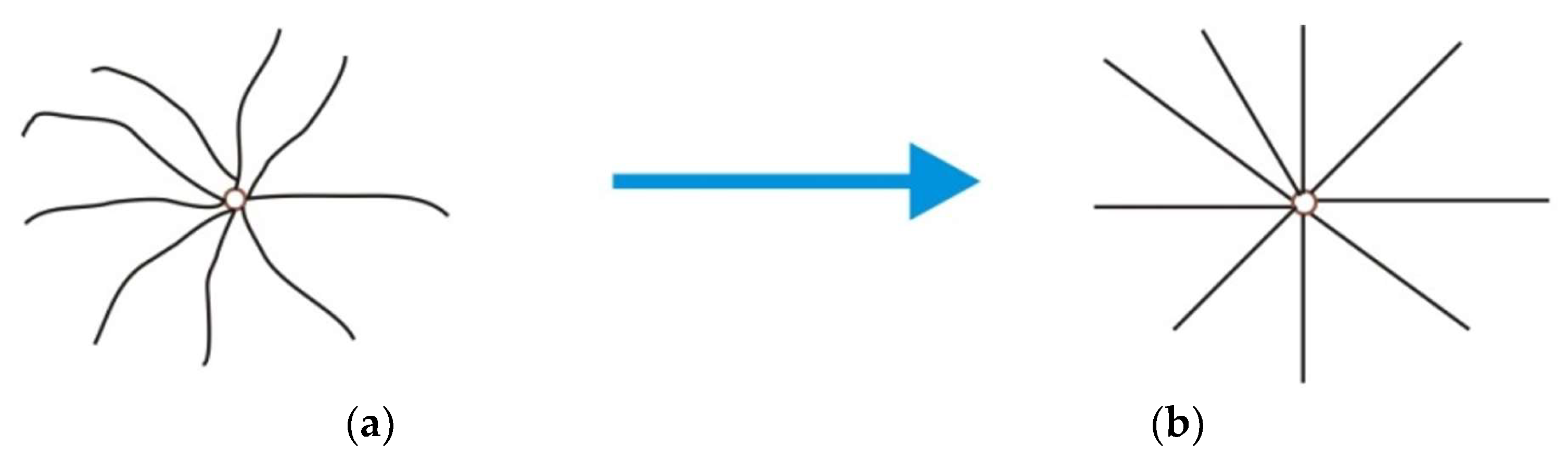
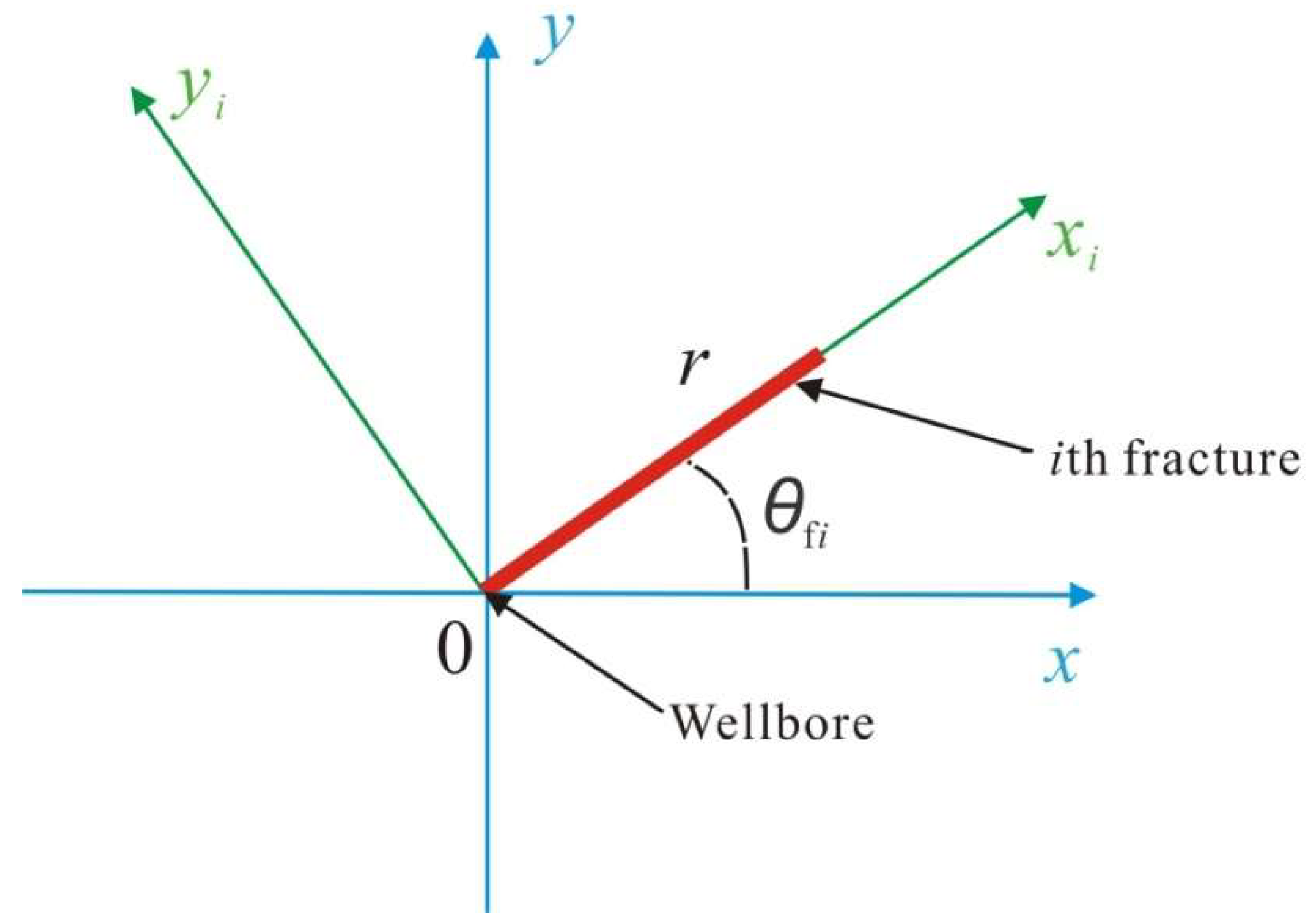
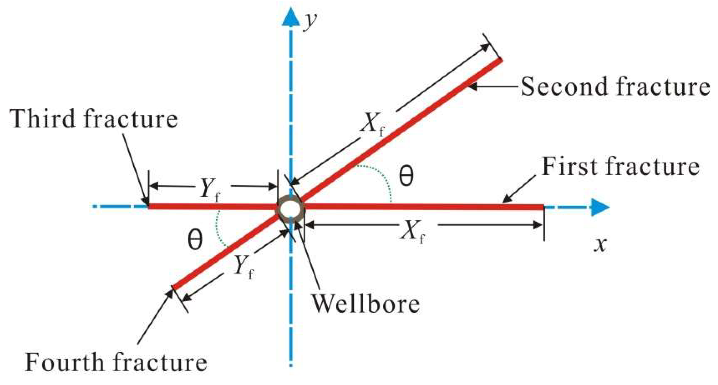
2. Physical Model
3. Mathematical Model
3.1. Flow Model for Stress-Sensitive Gas Reservoirs
3.2. Flow Model for Stress-Sensitive Hydraulic Fractures
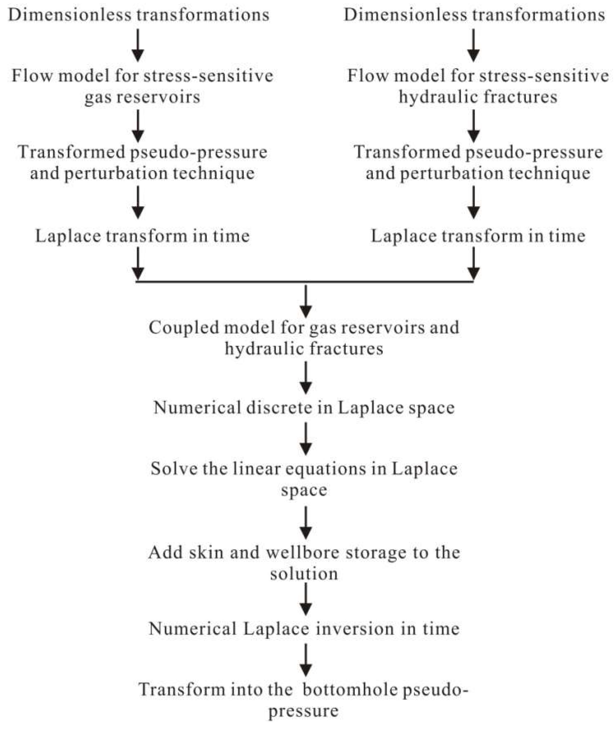
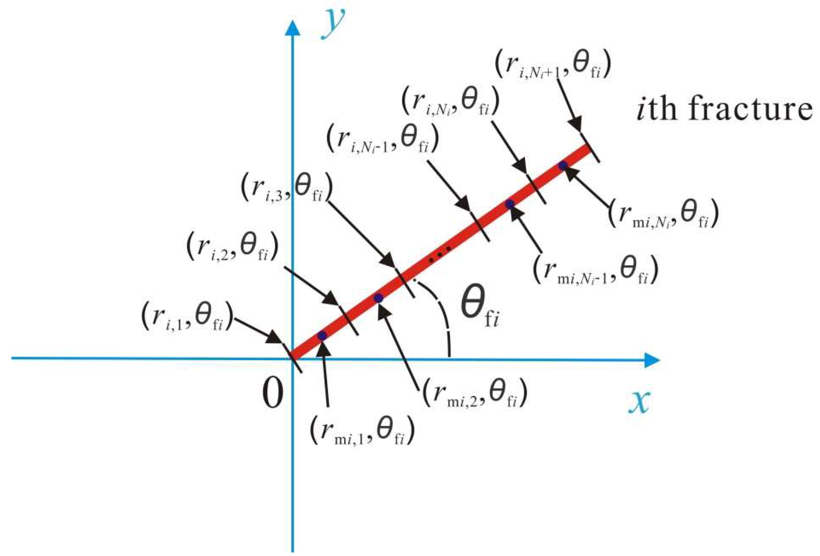
3.3. Coupled Discrete Model
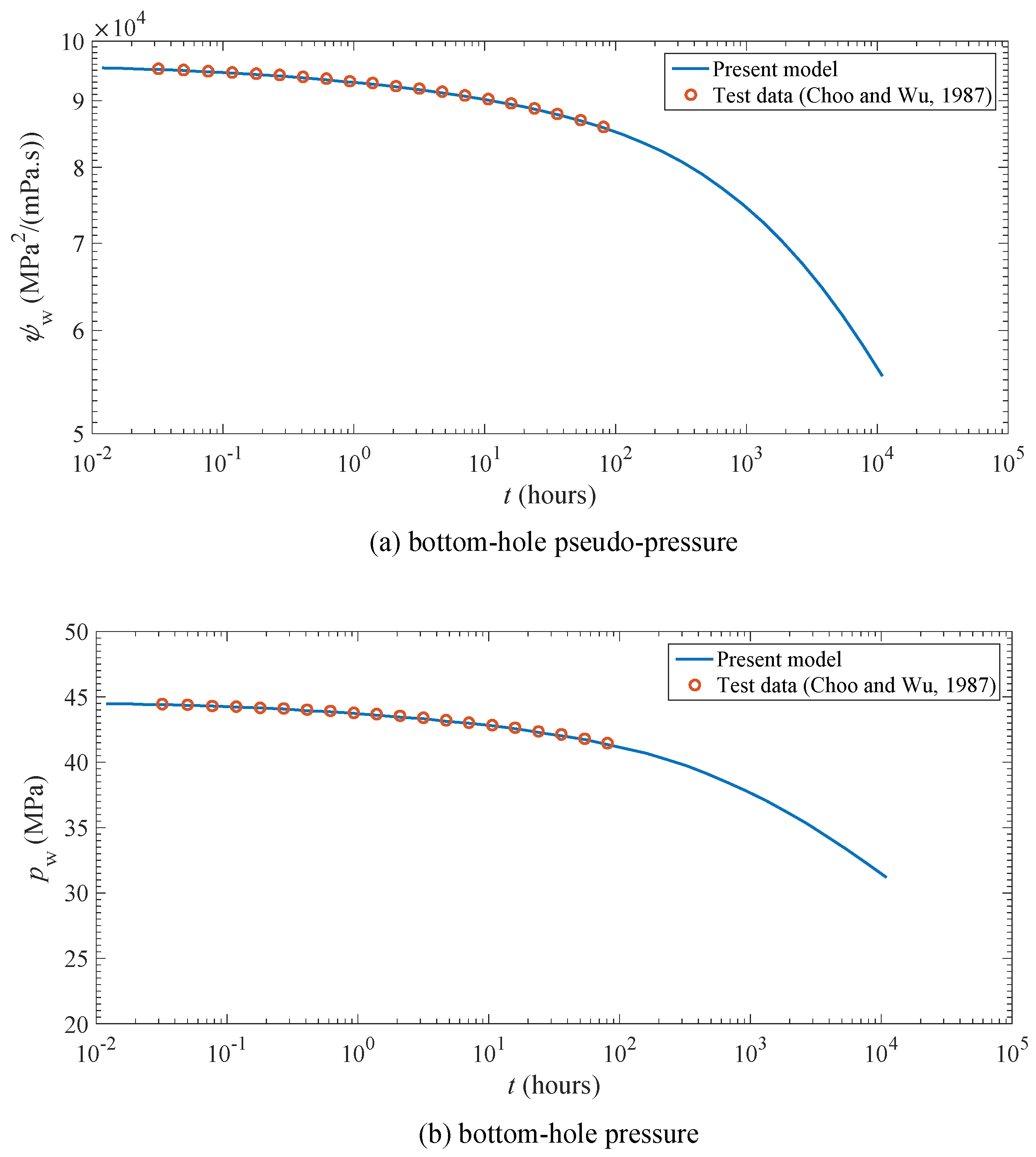
4. Model Validation and Application
5. Results and Analysis
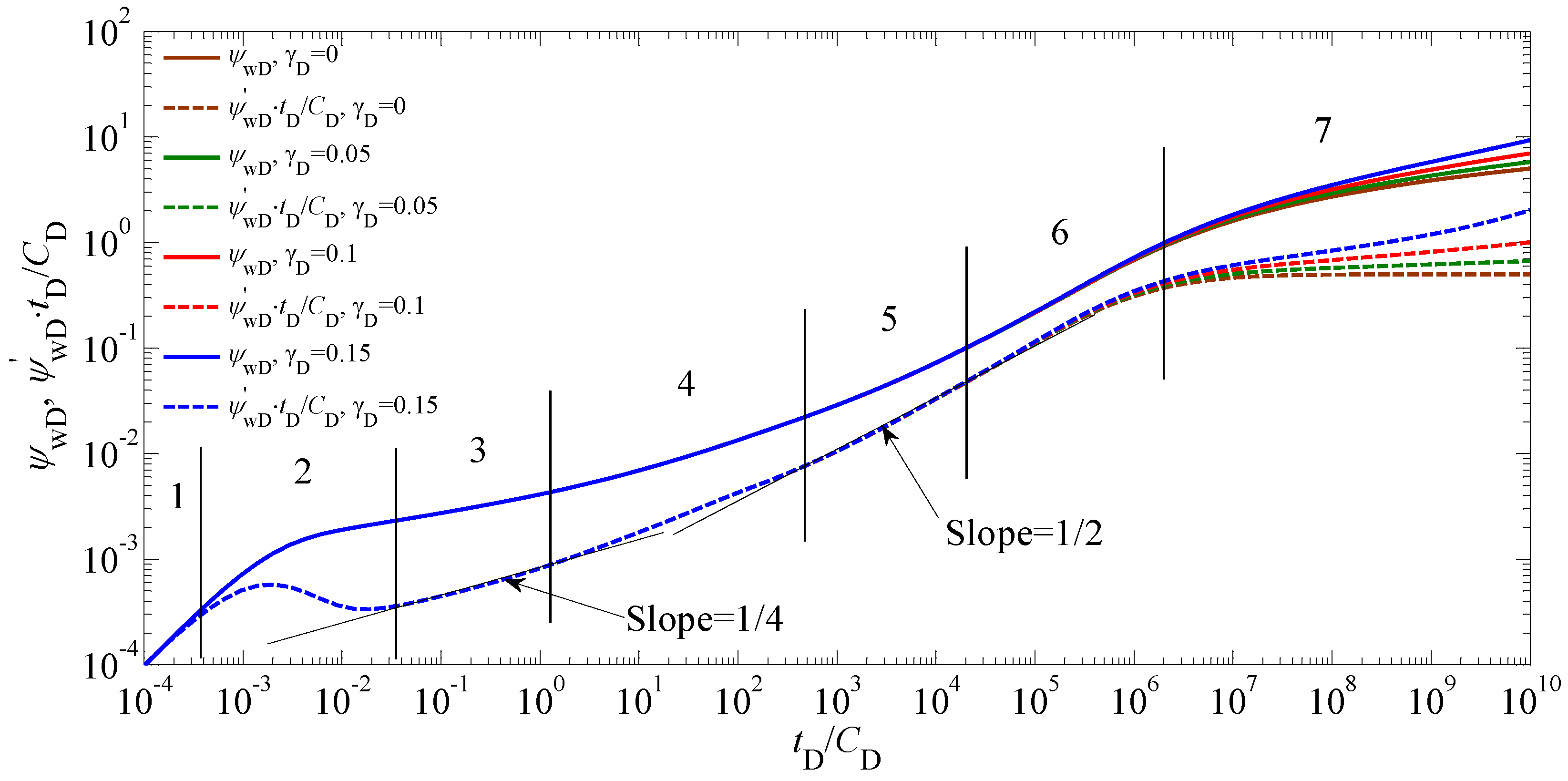
5.1. Type Curves and Flow Regimes
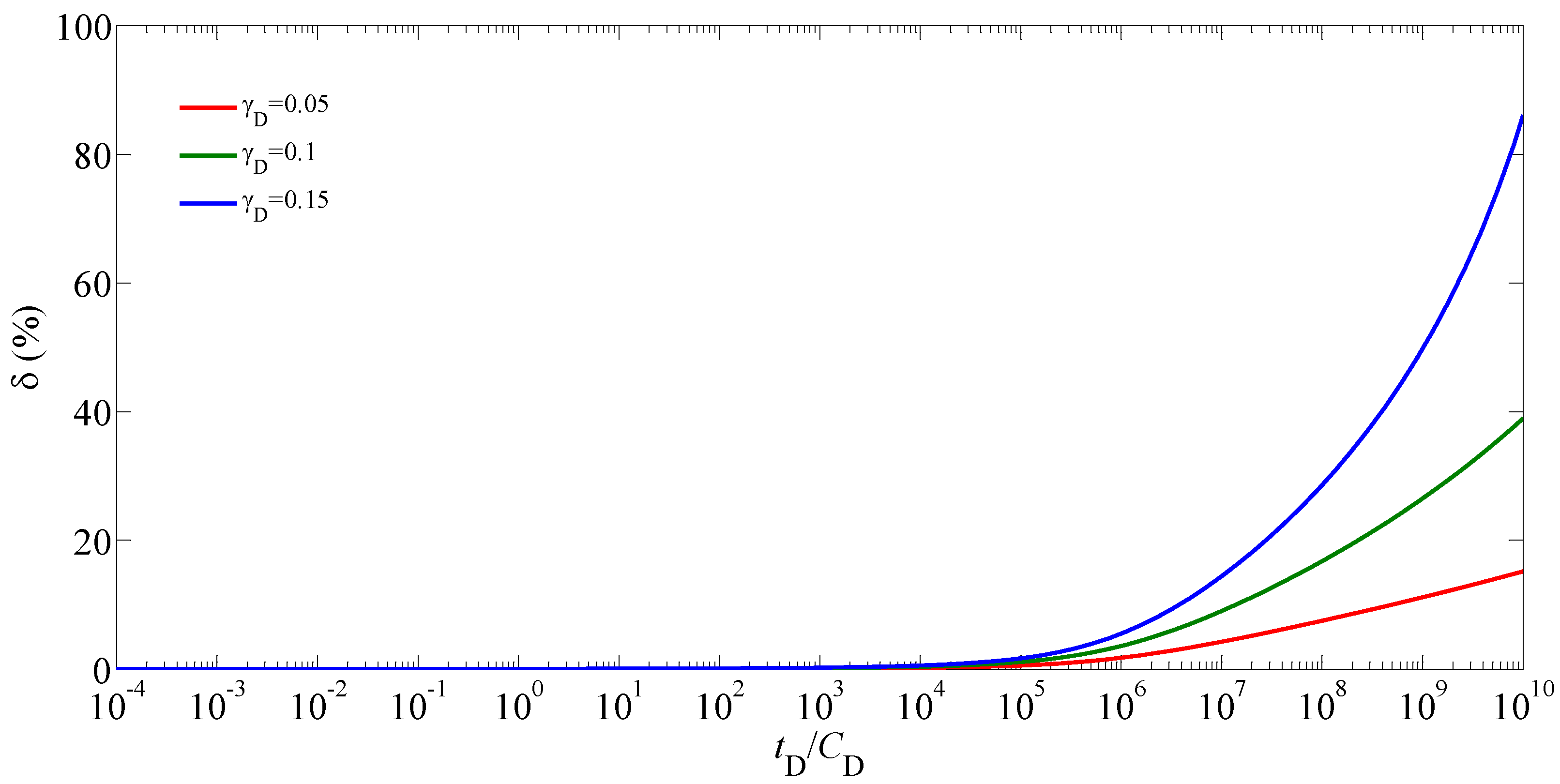
5.2. Sensitivity Analysis
6. Conclusions
Author Contributions
Funding
Conflicts of Interest
Appendix A. Symbol Description
| Nomenclature | |
| wellbore storage coefficient, | |
| fracture conductivity coefficient | |
| total compressibility of hydraulic fracture, | |
| total compressibility of gas reservoir, | |
| reservoir thickness, | |
| reservoir permeability, | |
| initial fracture permeability, | |
| initial reservoir permeability, | |
| length of the th hydraulic fracture, | |
| hydraulic-fracture number | |
| reservoir pressure, | |
| fracture pressure, | |
| initial reservoir pressure, | |
| pressure at standard condition, | |
| flow rate of point source, | |
| flow-rate density, | |
| production rate of the th hydraulic fracture, | |
| well production rate, | |
| radial distance, , | |
| wellbore radius, | |
| Laplace transform variable | |
| skin factor | |
| time, | |
| reservoir temperature, | |
| temperature at standard condition, | |
| fracture width, | |
| - and -coordinates, | |
| Z-factor of gas | |
| gas viscosity, | |
| permeability modulus, | |
| reservoir pseudo-pressure, | |
| fracture pseudo-pressure, | |
| initial reservoir pseudo-pressure, | |
| bottom-hole pseudo-pressure, | |
| dimensionless transformed reservoir pseudo-pressure | |
| dimensionless transformed fracture pseudo-pressure | |
| dimensionless transformed bottom-hole pseudo-pressure with wellbore storage and skin | |
| dimensionless transformed bottom-hole pseudo-pressure without wellbore storage and skin | |
| reservoir porosity | |
| fracture porosity | |
| polar angle, degree | |
| polar angle of the th hydraulic fracture, degree | |
| length of discrete segment of the th hydraulic fracture, | |
| Subscript | |
| dimensionless | |
| the jth discrete segment in the ith hydraulic fracture | |
| Superscript | |
| Laplace space | |
Appendix B. Pressure Distribution in a Gas Reservoir with a Vertical Fractured Well with Multiple Hydraulic Fractures Producing at a Constant Rate
Appendix C. Derivation of Dimensionless Model for Gas Flow within Stress-Sensitive Hydraulic Fractures
References
- Wang, Y.; Zhang, C.; Chen, T.; Ma, X. Modeling the Nonlinear Flow for a Multiple-fractured Horizontal Well with Multiple Finite-conductivity Fractures in Triple Media Carbonate Reservoir. J. Porous Media 2018, 21, 1283–1305. [Google Scholar] [CrossRef]
- Wang, Y.; Yi, X. Flow Modeling of Well Test Analysis for A Multiple-fractured Horizontal Well in Triple Media Carbonate Reservoir. Int. J. Nonlinear Sci. Numer. Simul. 2018, 19, 439–457. [Google Scholar] [CrossRef]
- Wang, Y.; Yi, X. Transient Pressure Behavior of a Fractured Vertical Well with A Finite-conductivity Fracture in Triple Media Carbonate Reservoir. J. Porous Media 2017, 20, 707–722. [Google Scholar] [CrossRef]
- Ren, J.; Guo, P. A Novel Semi-analytical Model for Finite-conductivity Multiple Fractured Horizontal Wells in Shale Gas Reservoirs. J. Nat. Gas Sci. Eng. 2015, 24, 35–51. [Google Scholar] [CrossRef]
- Ren, J.; Guo, P. Anomalous Diffusion Performance of Multiple Fractured Horizontal Wells in Shale Gas Reservoirs. J. Nat. Gas Sci. Eng. 2015, 26, 642–651. [Google Scholar] [CrossRef]
- Ren, J.; Guo, P. Nonlinear Seepage Model for Multiple Fractured Horizontal Wells with the Effect of the Quadratic Gradient Term. J. Porous Media 2018, 21, 223–239. [Google Scholar] [CrossRef]
- Ren, J.; Guo, P. A General Analytical Method for Transient Flow Rate with the Stress-sensitive Effect. J. Hydrol. 2018, 565, 262–275. [Google Scholar] [CrossRef]
- Ren, J.; Guo, P. Analytical Method for Transient Flow Rate with the Effect of the Quadratic Gradient Term. J. Pet. Sci. Eng. 2018, 162, 774–784. [Google Scholar] [CrossRef]
- Ren, J.; Guo, P.; Peng, S.; Ma, Z. Performance of Multi-stage Fractured Horizontal Wells with Stimulated Reservoir Volume in Tight Gas Reservoirs Considering Anomalous Diffusion. Environ. Earth Sci. 2018, 77, 768. [Google Scholar] [CrossRef]
- Ren, J.; Guo, P.; Guo, Z.; Wang, Z. A Lattice Boltzmann Model for simulating Gas Flow in Kerogen Pores. Transp. Porous Med. 2015, 106, 285–301. [Google Scholar] [CrossRef]
- Ren, J.; Guo, P.; Peng, S.; Yang, C. Investigation on Permeability of Shale Matrix using the Lattice Boltzmann Method. J. Nat. Gas Sci. Eng. 2016, 29, 169–175. [Google Scholar] [CrossRef]
- Ren, J.; Guo, P.; Guo, Z. Rectangular Lattice Boltzmann Equation for Gaseous Microscale Flow. Adv. Appl. Math. Mech. 2016, 8, 306–330. [Google Scholar] [CrossRef]
- Ren, J.; Guo, P. Lattice Boltzmann Simulation of Steady Flow in a Semi-Elliptical Cavity. Commun. Comput. Phys. 2017, 21, 692–717. [Google Scholar] [CrossRef]
- Ren, J.; Zheng, Q.; Guo, P.; Peng, S.; Wang, Z.; Du, J. Pore-scale Lattice Boltzmann Simulation of Two-component Shale Gas Flow. J. Nat. Gas Sci. Eng. 2019, 61, 46–70. [Google Scholar] [CrossRef]
- Ren, J.; Zheng, Q.; Guo, P.; Zhao, C. Lattice Boltzmann Model for Gas Flow through Tight Porous Media with Multiple Mechanisms. Entropy 2019, 21, 133. [Google Scholar] [CrossRef]
- Pedrosa, O.A. Pressure Transient Response in Stress-Sensitive Formations; SPE California Regional Meeting: Oakland, CA, USA, 1986. [Google Scholar]
- Zhang, Z.; He, S.; Liu, G.; Guo, X.; Mo, S. Pressure Buildup Behavior of Vertically Fractured Wells with Stress-sensitive Conductivity. J. Pet. Sci. Eng. 2014, 122, 48–55. [Google Scholar] [CrossRef]
- Wang, J.; Jia, A.; Wei, Y.; Qi, Y. Approximate Semi-analytical Modeling of Transient Behavior of Horizontal Well Intercepted by Multiple Pressure-dependent Conductivity Fractures in Pressure-sensitive Reservoir. J. Pet. Sci. Eng. 2017, 153, 157–177. [Google Scholar] [CrossRef]
- Gringarten, A.C.; Ramey, H.J.; Raghavan, J.R. Unsteady-state Pressure Distributions Created by a Well with a Single Infinite-conductivity Vertical Fracture. SPE J. 1974, 14, 347–360. [Google Scholar] [CrossRef]
- Cinco-Ley, H.; Samaniego, F.; Dominguez, N. Transient Pressure Behavior for a Well with a Finite-conductivity Vertical Fracture. SPE J. 1978, 18, 253–264. [Google Scholar]
- Bennett, C.O.; Reynolds, A.C.; Raghavan, R.; Elbel, J.L. Performance of Finite-conductivity, Vertically Fractured Wells in Single-layer Reservoirs. SPE Form. Eval. 1986, 1, 399–412. [Google Scholar] [CrossRef]
- Bennett, C.O.; Rosato, N.D.; Reynolds, A.C.; Raghavan, R. Influence of Fracture Heterogeneity and Wing Length on the Response of Vertically Fractured Wells. SPE J. 1983, 23, 219–230. [Google Scholar] [CrossRef]
- Rodriguez, F.; Cinco-Ley, H.; Samaniego, V.F. Evaluation of Fracture Asymmetry of Finite-conductivity Fractured Wells. SPE Prod. Eval. 1992, 7, 233–239. [Google Scholar] [CrossRef]
- Berumen, S.; Tiab, D.; Rodriguez, F. Constant Rate Solutions for a Fractured Well with an Asymmetric Fracture. J. Pet. Sci. Eng. 2000, 25, 49–58. [Google Scholar] [CrossRef]
- Tiab, D.; Lu, J.; Nguyen, H.; Owayed, J. Evaluation of Fracture Asymmetry of Finite-conductivity Fractured Wells. J. Energy Resour. Technol. 2010, 132, 1–7. [Google Scholar] [CrossRef]
- Wang, L.; Wang, X.; Li, J.; Wang, J. Simulation of Pressure Transient Behavior for Asymmetrically Finite-conductivity Fractured Wells in Coal Reservoirs. Transp. Porous Media 2013, 97, 353–372. [Google Scholar] [CrossRef]
- Wang, L.; Wang, X. Type Curves Analysis for Asymmetrically Fractured Wells. J. Energy Resour. Technol. 2014, 136, 023101. [Google Scholar] [CrossRef]
- Fisher, M.K.; Wright, C.A.; Davidson, B.M.; Goodwin, A.K.; Fielder, E.O.; Buckler, W.S.; Steinsberger, N.P. Integrating Fracture Mapping Technologies to Improve Stimulations in the Barnett Shale. SPE Prod. Facil. 2005, 20, 85–93. [Google Scholar] [CrossRef]
- Mayerhofer, M.J.; Lolon, E.P.; Youngblood, J.E.; Heinze, J.R. Integration of Microseismic-Fracture-Mapping Results with Numerical Fracture Network Production Modeling in the Barnett Shale; SPE Annual Technical Conference and Exhibition: San Antonio, TX, USA, 2006. [Google Scholar]
- Fan, Z.Q.; Jin, Z.H.; Johnson, S.E. Oil-gas Transformation Induced Subcritical Crack Propagation and Coalescence in Petroleum Source Rocks. Int. J. Fract. 2014, 185, 187–194. [Google Scholar] [CrossRef]
- Ren, J.; Guo, P. Nonlinear Flow Model of Multiple Fractured Horizontal Wells with Stimulated Reservoir Volume including the Quadratic Gradient Term. J. Hydrol. 2017, 554, 155–172. [Google Scholar] [CrossRef]
- Shaoul, J.R.; Behr, A.; Mtchedlishvili, G. Developing a Tool for 3D Reservoir Simulation of Hydraulically Fractured Wells. SPE Reservoir Eval. Eng. 2007, 10, 50–59. [Google Scholar] [CrossRef]
- Restrepo, D.P.; Tiab, D. Multiple fractures transient response. In Proceedings of the SPE Latin American and Caribbean Petroleum Engineering Conference, Cartagena de Indias, Colombia, 31 May–3 June 2009. [Google Scholar]
- Wang, L.; Wang, X.; Luo, E.; Wang, J. Analytical Modeling of Flow Behavior for Wormholes in Naturally Fractured-vuggy Porous Media. Transp. Porous Media 2014, 105, 539–558. [Google Scholar] [CrossRef]
- Ren, J.; Guo, P. Performance of Vertical Fractured Wells with Multiple Finite-conductivity Fractures. J. Geophys. Eng. 2015, 12, 978–987. [Google Scholar] [CrossRef]
- Luo, W.; Tang, C. Pressure-transient Analysis of Multiwing Fractures Connected to a Vertical Wellbore. SPE J. 2015, 20, 360–367. [Google Scholar] [CrossRef]
- Wang, H.T. Performance of Multiple Fractured Horizontal Wells in Shale Gas Reservoirs with Consideration of Multiple Mechanisms. J. Hydrol. 2014, 510, 299–312. [Google Scholar] [CrossRef]
- Li, X.P.; Cao, L.N.; Luo, C.; Zhang, B.; Zhang, J.Q.; Tan, X.H. Characteristics of Transient Production Rate Performance of Horizontal Well in Fractured Tight Gas Reservoirs with Stress-sensitivity Effect. J. Pet. Sci. Eng. 2017, 158, 92–106. [Google Scholar] [CrossRef]
- Ozkan, E. Performance of Horizontal Wells. Ph.D. Thesis, University of Tulsa, Tulsa, OK, USA, 1988. [Google Scholar]
- Wan, J. Well Models of Hydraulically Fractured Horizontal Wells. Master’s Thesis, Stanford University, Palo Alto, CA, USA, 1999. [Google Scholar]
- Van Everdingen, A.F.; Hurst, W. The Application of the Laplace Transformation to Flow Problems in Reservoirs. Trans. AIME 1949, 186, 305–324. [Google Scholar] [CrossRef]
- Stehfest, H. Numerical Inversion of Laplace Transforms. Commun. ACM 1970, 13, 47–49. [Google Scholar] [CrossRef]
- Akanji, L.T.; Falade, G.K. Closed-Form Solution of Radial Transport of Tracers in Porous Media Influenced by Linear Drift. Energies 2019, 12, 29. [Google Scholar] [CrossRef]
- Choo, Y.K.; Wu, C.H. Transient Pressure Behavior of Multiple-fractured Gas Wells. In Proceedings of the SPE/DOE Low Permeability Reservoirs Symposium, Denver, CO, USA, 18–19 May 1987. [Google Scholar]


| Nomenclature | Definition |
|---|---|
| Parameter | Value |
|---|---|
| Reservoir thickness, , | |
| Reservoir porosity, | |
| Initial reservoir permeability, , | |
| Initial fracture permeability, , | |
| Initial reservoir pressure, , | |
| Initial reservoir pseudo-pressure, , | 9.6321 × 10⁴ |
| Total compressibility, , | |
| Wellbore radius, , | |
| Gas viscosity, , | |
| Reservoir temperature, , | |
| Fracture width, , | |
| Well production rate, , | |
| Polar angles of the hydraulic fractures, , degree | |
| Lengths of the hydraulic fractures, , |
© 2019 by the authors. Licensee MDPI, Basel, Switzerland. This article is an open access article distributed under the terms and conditions of the Creative Commons Attribution (CC BY) license (http://creativecommons.org/licenses/by/4.0/).
Share and Cite
Guo, P.; Sun, Z.; Peng, C.; Chen, H.; Ren, J. Transient-Flow Modeling of Vertical Fractured Wells with Multiple Hydraulic Fractures in Stress-Sensitive Gas Reservoirs. Appl. Sci. 2019, 9, 1359. https://doi.org/10.3390/app9071359
Guo P, Sun Z, Peng C, Chen H, Ren J. Transient-Flow Modeling of Vertical Fractured Wells with Multiple Hydraulic Fractures in Stress-Sensitive Gas Reservoirs. Applied Sciences. 2019; 9(7):1359. https://doi.org/10.3390/app9071359
Chicago/Turabian StyleGuo, Ping, Zhen Sun, Chao Peng, Hongfei Chen, and Junjie Ren. 2019. "Transient-Flow Modeling of Vertical Fractured Wells with Multiple Hydraulic Fractures in Stress-Sensitive Gas Reservoirs" Applied Sciences 9, no. 7: 1359. https://doi.org/10.3390/app9071359
APA StyleGuo, P., Sun, Z., Peng, C., Chen, H., & Ren, J. (2019). Transient-Flow Modeling of Vertical Fractured Wells with Multiple Hydraulic Fractures in Stress-Sensitive Gas Reservoirs. Applied Sciences, 9(7), 1359. https://doi.org/10.3390/app9071359