3D Strain and Elasticity Measurement of Layered Biomaterials by Optical Coherence Elastography based on Digital Volume Correlation and Virtual Fields Method


Abstract
:Featured Application
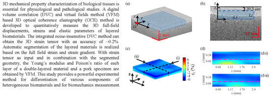
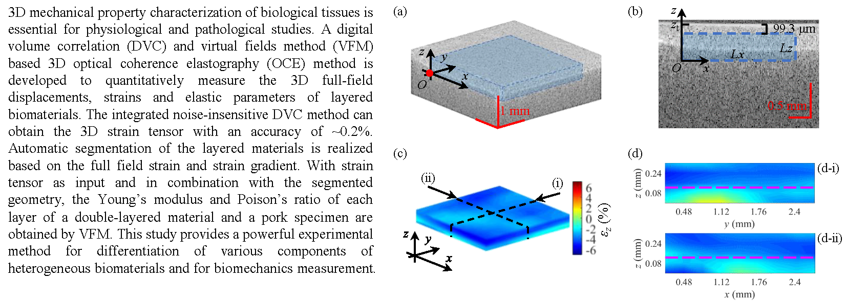
Abstract
1. Introduction
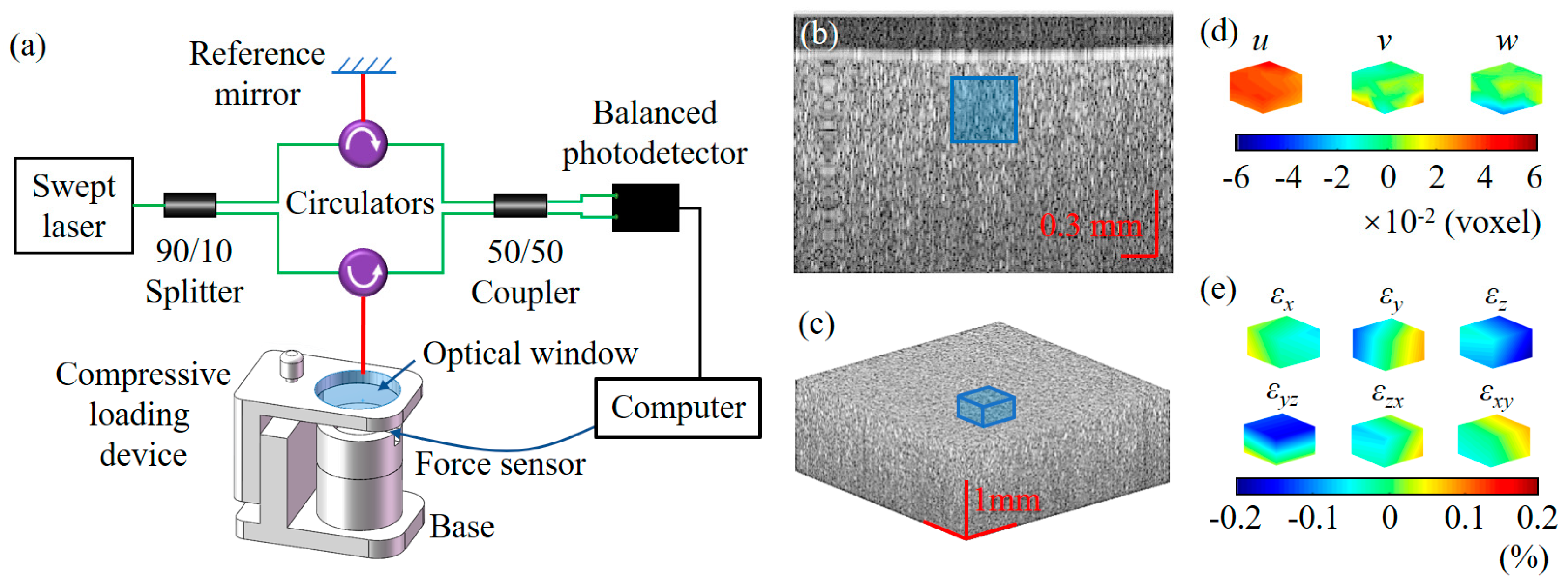
2. Equipment and Methods
2.1. 3D Strain Measurement by OCT Imaging and DVC
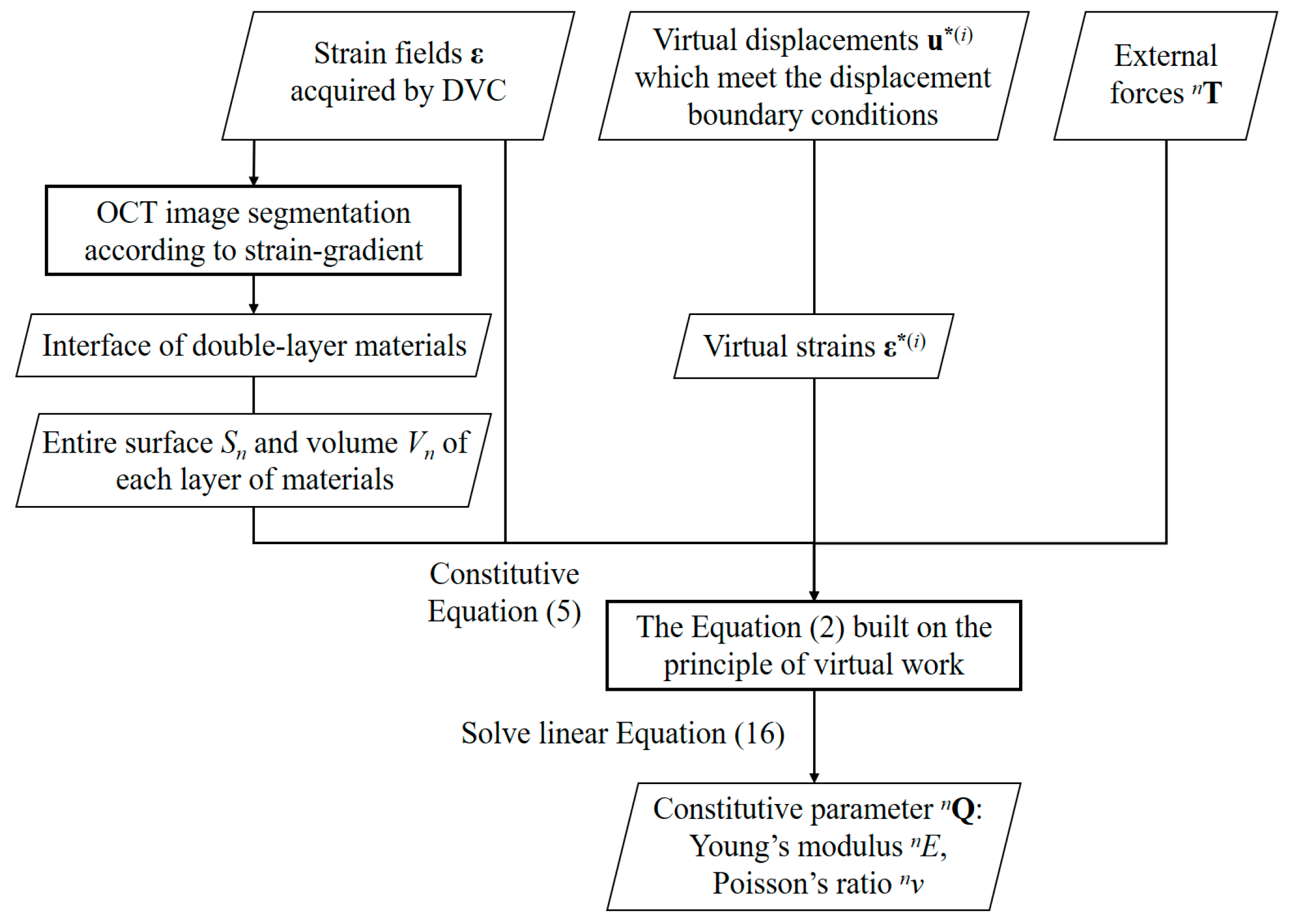
2.2. VFM
3. Experiments
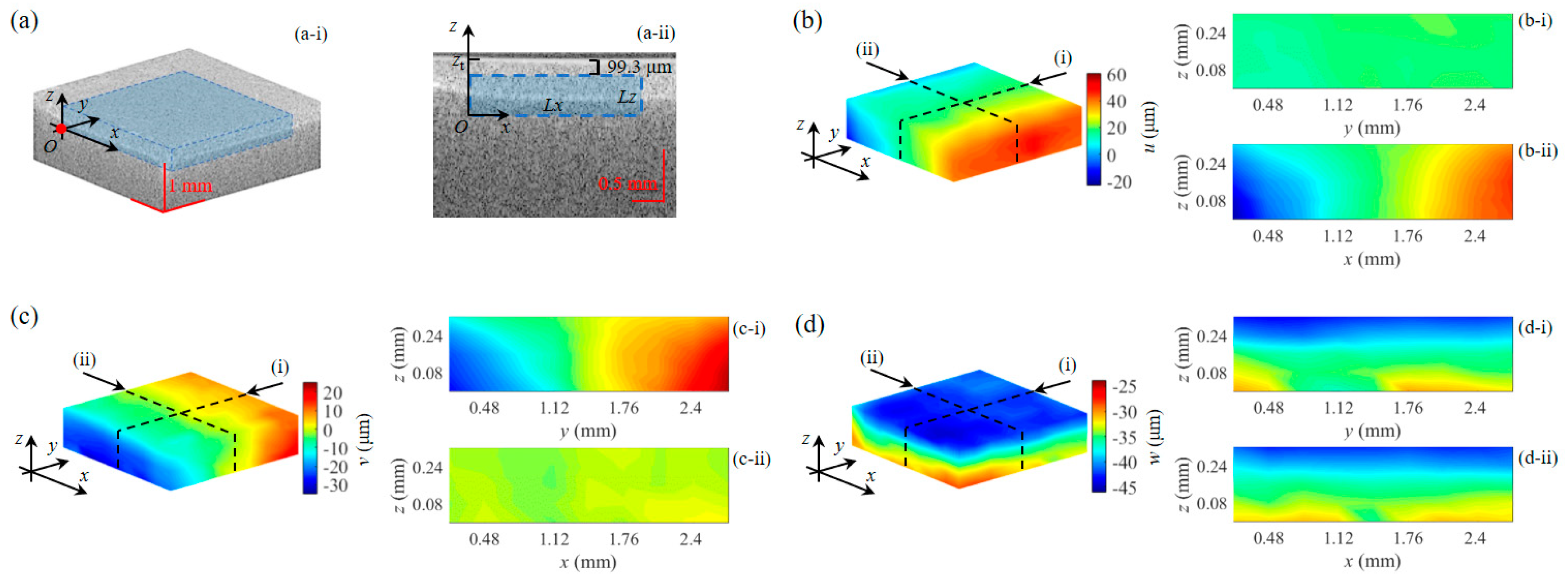
3.1. Strain and Young’s Modulus Measurement of a Homogeneous Phantom
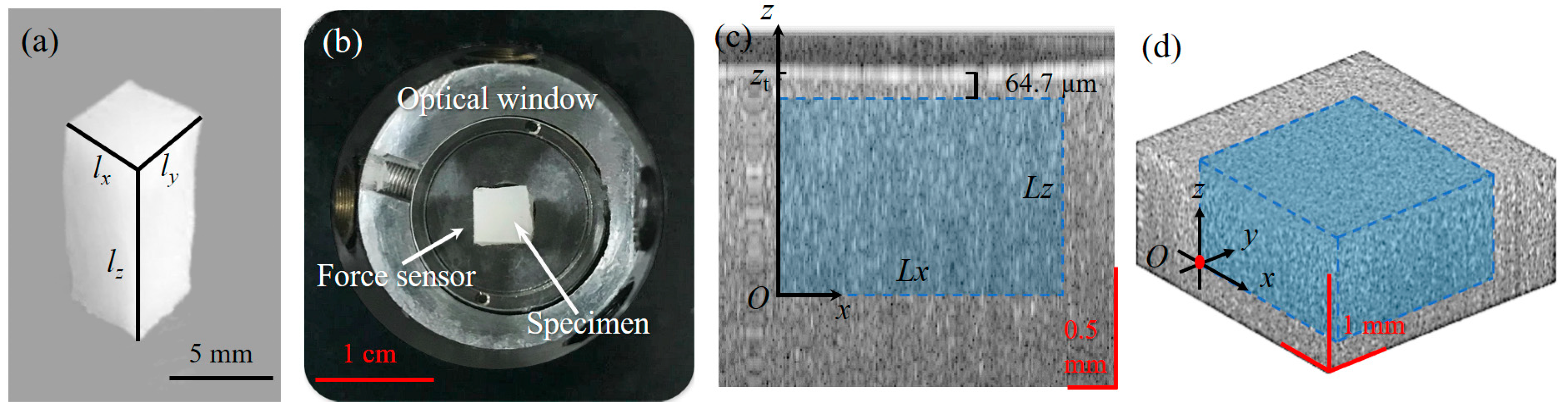
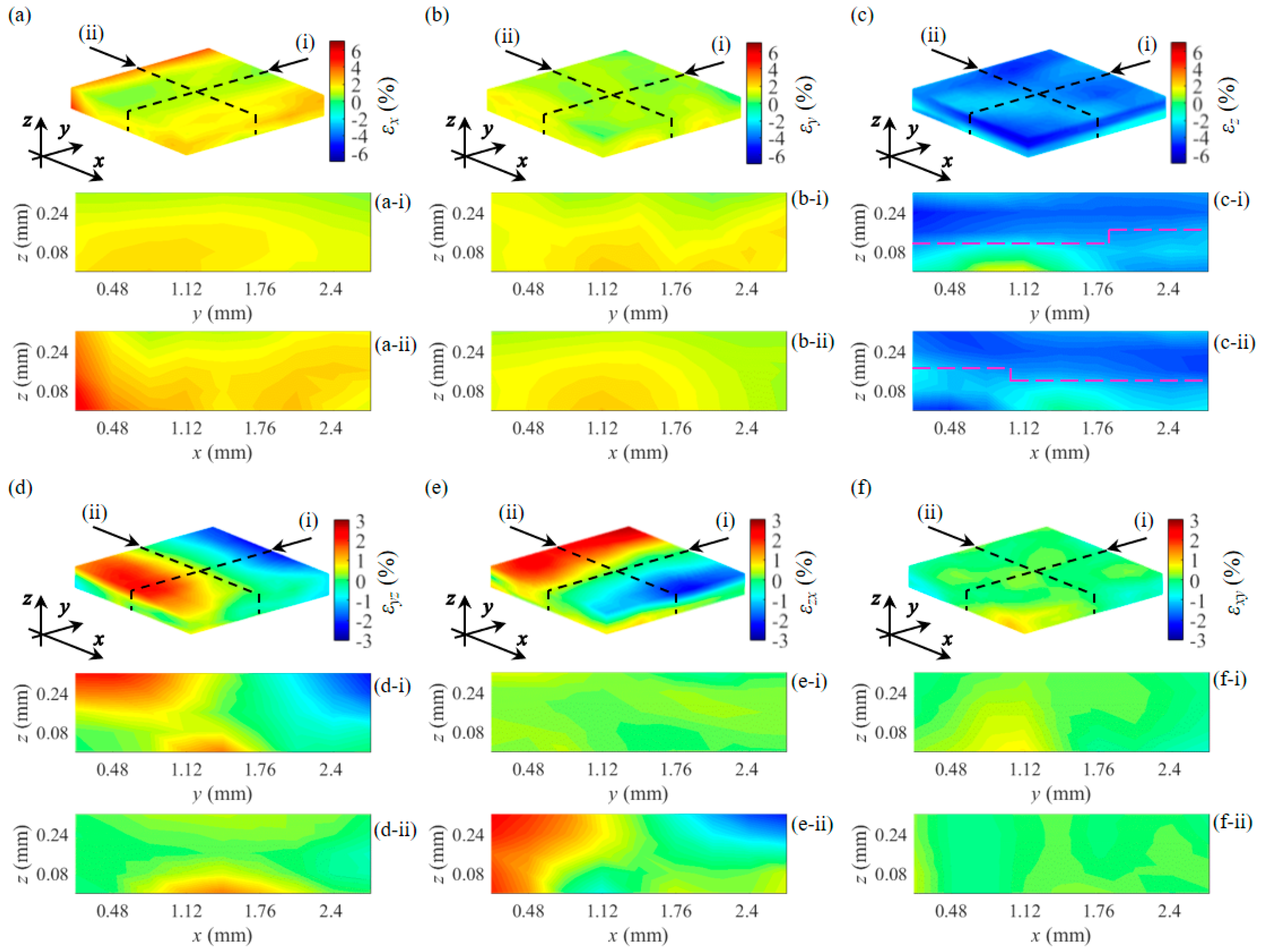
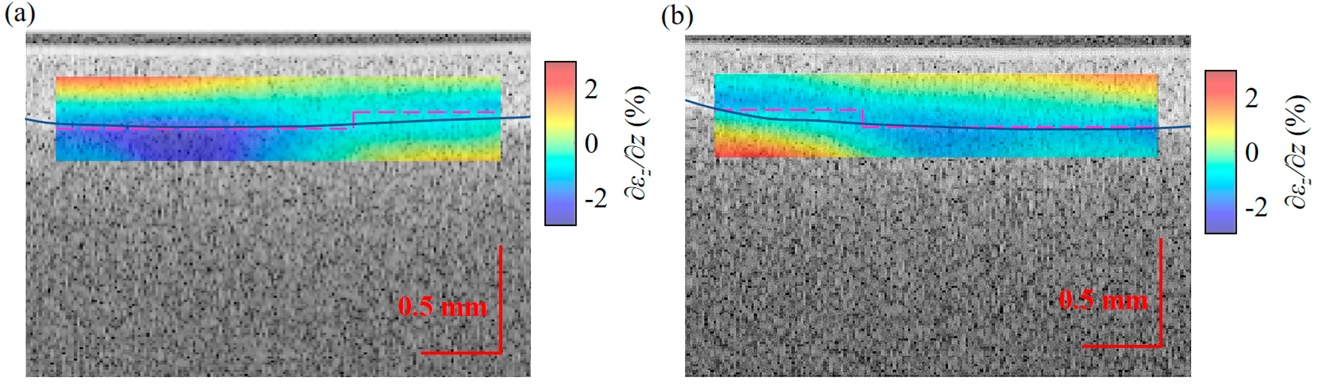
3.2. Strain and Young’s Modulus Measurement of a Double-Layer Phantom
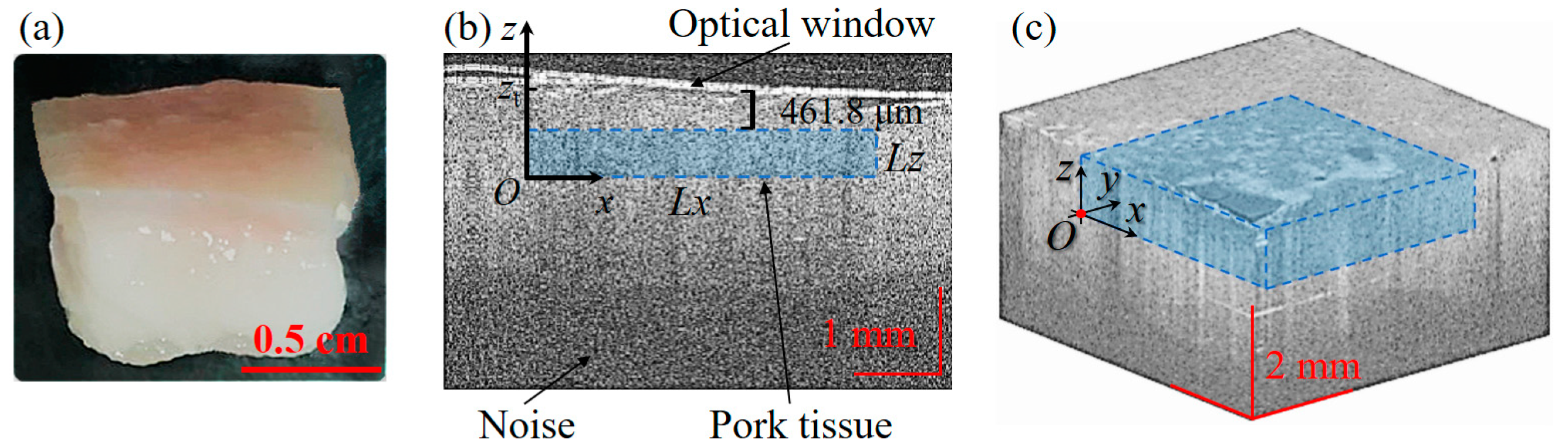
3.3. Strain and Young’s Modulus Measurement of Pork
4. Discussion
5. Conclusions
Author Contributions
Funding
Acknowledgments
Conflicts of Interest
References
- Larin, K.V.; Sampson, D.D. Optical coherence elastography—OCT at work in tissue biomechanics [Invited]. Biomed. Opt. Express 2017, 8, 1172–1202. [Google Scholar] [CrossRef]
- Wang, S.; Larin, K.V. Optical coherence elastography for tissue characterization: A review. J. Biophotonics 2015, 8, 279–302. [Google Scholar] [CrossRef]
- Wang, R.K.; Ma, Z.S.; Kirkpatrick, J. Tissue Doppler optical coherence elastography for real time strain rate and strain mapping of soft tissue. Appl. Phys. Lett. 2006, 89, 144103. [Google Scholar] [CrossRef]
- Wang, R.K.; Kirkpatrick, S.; Hinds, M. Phase-sensitive optical coherence elastography for mapping tissue microstrains in real time. Appl. Phys. Lett. 2007, 90, 164105. [Google Scholar] [CrossRef]
- Schmitt, J.M. OCT elastography: Imaging microscopic deformation and strain of tissue. Opt. Express 1998, 3, 199–211. [Google Scholar] [CrossRef] [PubMed]
- Luo, Z.; Wang, Z.; Yuan, Z.; Du, C.; Pan, Y. Optical coherence Doppler tomography quantifies laser speckle contrast imaging for blood flow imaging in the rat cerebral cortex. Opt. Lett. 2008, 33, 1156–1158. [Google Scholar] [CrossRef]
- Rogowska, J.; Patel, N.A.; Fujimoto, J.G.; Brezinski, M.E. Optical coherence tomographic elastography technique for measuring deformation and strain of atherosclerotic tissues. Heart 2004, 90, 556–562. [Google Scholar] [CrossRef] [PubMed] [Green Version]
- Chan, R.C.; Chau, A.H.; Karl, W.C.; Nadkarni, S.; Khalil, A.S.; Iftimia, N.; Shishkov, M.; Tearney, G.J.; Mofrad, M.R.K.; Bouma, B.E. OCT-based arterial elastography: Robust estimation exploiting tissue biomechanics. Opt. Express 2004, 12, 4558–4572. [Google Scholar] [CrossRef]
- Khalil, A.S.; Chan, R.C.; Chau, A.H.; Bouma, B.E.; Mofrad, M.R.K. Tissue Elasticity Estimation with Optical Coherence Elastography: Toward Mechanical Characterization of In Vivo Soft Tissue. Ann. Biomed. Eng. 2005, 33, 1631–1639. [Google Scholar] [CrossRef] [PubMed]
- Rogowska, J.; Patel, N.; Plummer, S.; Brezinski, M.E. Quantitative optical coherence tomographic elastography: Method for assessing arterial mechanical properties. Br. J. Radiol. 2006, 79, 707–711. [Google Scholar] [CrossRef] [PubMed]
- Sun, C.; Standish, B.; Vuong, B.; Wen, X.Y.; Yang, V. Digital image correlation-based optical coherence elastography. J. Biomed. Opt. 2013, 18, 121515. [Google Scholar] [CrossRef]
- Chu, T.C.; Ranson, W.F.; Sutton, M.A. Applications of digital-image-correlation techniques to experimental mechanics. Exp. Mech. 1985, 25, 232–244. [Google Scholar] [CrossRef]
- Fu, J.; Pierron, F.; Ruiz, P.D. Elastic stiffness characterization using three-dimensional full-field deformation obtained with optical coherence tomography and digital volume correlation. J. Biomed. Opt. 2013, 18, 121512. [Google Scholar] [CrossRef] [Green Version]
- Fu, J.; Haghighi-Abayneh, M.; Pierron, F.; Ruiz, P.D. Depth-resolved full-field measurement of corneal deformation by optical coherence tomography and digital volume correlation. Exp. Mech. 2016, 56, 1203–1217. [Google Scholar] [CrossRef]
- Nahas, A.; Bauer, M.; Roux, S.; Boccara, A.C. 3D static elastography at the micrometer scale using Full Field OCT. Biomed. Opt. Express 2013, 4, 2138–2149. [Google Scholar] [CrossRef] [PubMed] [Green Version]
- Acosta Santamaría, V.A.; García, M.F.; Molimard, J.; Avril, S. Three-Dimensional Full-Field Strain Measurements across a Whole Porcine Aorta Subjected to Tensile Loading Using Optical Coherence Tomography–Digital Volume Correlation. Front. Mech. Eng. 2018, 4, 3. [Google Scholar] [CrossRef]
- Girard, M.J.; Strouthidis, N.G.; Desjardins, A.; Mari, J.M.; Ethier, E.R. In vivo optic nerve head biomechanics: Performance testing of a three-dimensional tracking algorithm. J. R. Soc. Interface 2013, 10, 20130459. [Google Scholar] [CrossRef]
- Zhang, L.; Thakku, S.G.; Beotra, M.R.; Baskaran, M.; Aung, T.; Goh, J.C.H.; Strouthidis, N.G.; Girard, M.J.A. Verification of a virtual fields method to extract the mechanical properties of human optic nerve head tissues in vivo. Biomech. Model. Mechanobiol. 2016, 16, 871–887. [Google Scholar] [CrossRef] [PubMed]
- Bay, B.K.; Smith, T.S.; Fyhrie, D.P.; Saad, M. Digital volume correlation: Three-dimensional strain mapping using X-ray tomography. Exp. Mech. 1999, 39, 217–226. [Google Scholar] [CrossRef]
- Pan, B.; Xie, H.; Wang, Z. Equivalence of digital image correlation criteria for pattern matching. Appl. Opt. 2010, 49, 5501–5509. [Google Scholar] [CrossRef]
- Pan, B.; Wang, B.; Wu, D.; Lubineau, G. An efficient and accurate 3D displacements tracking strategy for digital volume correlation. Opt. Lasers Eng. 2014, 58, 126–135. [Google Scholar] [CrossRef]
- Zauel, R.; Yeni, Y.N.; Bay, B.K.; Dong, X.N.D.; Fyhrie, P. Comparison of the linear finite element prediction of deformation and strain of human cancellous bone to 3D digital volume correlation measurements. J. Biomech. Eng. 2006, 128, 1–6. [Google Scholar] [CrossRef] [PubMed]
- Pierron, F.; Grédiac, M. The Virtual Fields Method; Springer: New York, NY, USA, 2012; p. 57. [Google Scholar]
- Wu, J. Elasticity; Higher Education Press: Beijing, China, 2001; p. 34. [Google Scholar]
- Zaitsev, V.Y.; Matveev, L.A.; Matveyev, A.L.; Gelikonov, G.V.; Gelikonov, V.M. Elastographic mapping in optical coherence tomography using an unconventional approach based on correlation stability. J. Biomed. Opt. 2014, 19, 021107. [Google Scholar] [CrossRef]
- Zaitsev, V.Y.; Matveev, L.A.; Matveyev, A.L.; Gelikonov, G.V.; Gelikonov, V.M. A model for simulating speckle-pattern evolution based on close to reality procedures used in spectral-domain OCT. Laser Phys. Lett. 2014, 11, 105601. [Google Scholar] [CrossRef] [Green Version]
- Yeung, C.C.; Holmes, D.F.; Thomason, H.A.; Stephenson, C.; Derby, B.; Hardman, M.J. An ex vivo porcine skin model to evaluate pressure-reducing devices of different mechanical properties used for pressure ulcer prevention. Wound Repair Regen. 2016, 24, 1089–1096. [Google Scholar] [CrossRef] [Green Version]
- Gu, Y.; Fei, G.; Zhang, H.; Liu, F. Test and analysis of friction coefficient on glass floor. Glass 2018, 3, 11–17. [Google Scholar]
- Piederrière, Y.; Boulvert, F.; Cariou, J.; Le Jeune, B.; Guern, Y.; Le, G. BrunBackscattered speckle size as a function of polarization: Influence of particle-size and concentration. Opt. Express 2005, 13, 5030–5039. [Google Scholar] [CrossRef] [PubMed]
- Lamouche, G.; Bisaillon, C.E.; Vergnole, S.; Monchalin, J.P. On the speckle Size in Optical Coherence Tomography. Proc. SPIE 2008. [Google Scholar] [CrossRef]
- Lamouche, G.; Bisaillon, C.E.; Maciejko, R.; Dufour, M.; Monchalin, J.P. Speckle size in optical coherence tomography. Proc. SPIE 2007. [Google Scholar] [CrossRef]
- Kurokawa, K.; Makita, S.; Hong, Y.J.; Yasuno, Y. Two-dimensional micro-displacement measurement for laser coagulation using optical coherence tomography. Biomed. Opt. Express 2015, 6, 170–190. [Google Scholar] [CrossRef]
- Kurokawa, K.; Makita, S.; Hong, Y.J.; Yasuno, Y. In-plane and out-of-plane tissue micro-displacement measurement by correlation coefficients of optical coherence tomography. Opt. Lett. 2015, 40, 2153–2156. [Google Scholar] [CrossRef] [PubMed]
- Wijesinghe, P.; Chin, L.; Kennedy, B.F. Strain tensor imaging in compression optical coherence elastography. IEEE J. Sel. Top. Quantum Electron. 2019, 25. [Google Scholar] [CrossRef]


| Young’s Moduli | Tensile Tests | VMF | Relative Errors |
|---|---|---|---|
| E1 (kPa) | 462.1 | 439.7 | 4.8% |
| E2 (kPa) | 120.8 | 121.4 | 0.5% |
© 2019 by the authors. Licensee MDPI, Basel, Switzerland. This article is an open access article distributed under the terms and conditions of the Creative Commons Attribution (CC BY) license (http://creativecommons.org/licenses/by/4.0/).
Share and Cite
Meng, F.; Zhang, X.; Wang, J.; Li, C.; Chen, J.; Sun, C. 3D Strain and Elasticity Measurement of Layered Biomaterials by Optical Coherence Elastography based on Digital Volume Correlation and Virtual Fields Method. Appl. Sci. 2019, 9, 1349. https://doi.org/10.3390/app9071349
Meng F, Zhang X, Wang J, Li C, Chen J, Sun C. 3D Strain and Elasticity Measurement of Layered Biomaterials by Optical Coherence Elastography based on Digital Volume Correlation and Virtual Fields Method. Applied Sciences. 2019; 9(7):1349. https://doi.org/10.3390/app9071349
Chicago/Turabian StyleMeng, Fanchao, Xinya Zhang, Jingbo Wang, Chuanwei Li, Jinlong Chen, and Cuiru Sun. 2019. "3D Strain and Elasticity Measurement of Layered Biomaterials by Optical Coherence Elastography based on Digital Volume Correlation and Virtual Fields Method" Applied Sciences 9, no. 7: 1349. https://doi.org/10.3390/app9071349