Article

Smart Cyber-Physical Manufacturing: Extended and Real-Time Optimization of Logistics Resources in Matrix Production

1
Institute of Logistics, University of Miskolc, 3515 Miskolc, Hungary
2
Institute of Logistics and Material Handling Systems, Otto-von-Guericke University Magdeburg, 39106 Magdeburg, Germany
3
Department of Mechanical Engineering, Universidad Central “Marta Abreu” de las Villas, 54830 Santa Clara, Cuba
4
Department of Agricultural Economics and Management, Zhejiang University, Hangzhou 310029, China
*
Author to whom correspondence should be addressed.
Appl. Sci. 2019, 9(7), 1287; https://doi.org/10.3390/app9071287
Submission received: 13 February 2019 / Revised: 19 March 2019 / Accepted: 22 March 2019 / Published: 27 March 2019

Abstract

:
In the context of Industry 4.0, the matrix production concept represents revolutionary solutions from a technological and logistics point of view. In a matrix production system, flexible, configurable production and assembly cells are arranged in a grid layout, and the in-plant supply is based on autonomous vehicles. Adaptable and flexible material handling solutions are required to perform the dynamically changing supply-demands of standardized and categorized manufacturing and assembly cells. Within the frame of this paper, the authors describe the in-plant supply process of matrix production and the optimization potential in these processes. After a systematic literature review, this paper introduces the structure of matrix production as a cyber-physical system focusing on logistics aspects. A mathematical model of this in-plant supply process is described including extended and real-time optimization from routing, assignment, and scheduling points of view. The optimization problem described in the model is an NP-hard problem. There are no known efficient analytical methods to find the best solution for this kind of problem; therefore, we use heuristics to find a suitable solution for the above-described problem. Next, a sequential black hole–floral pollination heuristic algorithm is described. The scenario analysis, which focuses on the clustering and routing aspects of supply demands in a matrix production system, validates the model and evaluates its performance to increase cost-efficiency and warrants environmental awareness of the in-plant supply in matrix production.

Graphical Abstract

1. Introduction

Production companies have to apply the solutions of cyber-physical systems to improve their availability, efficiency, reliability, and productivity. The ever-changing manufacturing industry requires the improvement of these attributes. Statistical surveys suggest that by the end of 2019, about 75% of large manufacturing companies will update their operations with Internet of Things solutions [1] and transform their conventional manufacturing environment to cyber-physical systems. The integration of IoT solutions leads to hyperconnected value chains, where not only manufacturing but also the related supply chain and logistics processes are operating in a cyber-physical environment.
KUKA AG (a German manufacturer of industrial robots and solutions having 25 subsidiaries worldwide) created a new versatile solution that compensates for peak capacity utilization or bottlenecks in resources. In a matrix production system, configurable production or assembly cells are arranged in a grid layout, and the in-plant supply is based on electric automated guided vehicles [2]. The matrix production system integrates a wide range of Internet of Things technologies and solutions, like standardized configurable production and assembly cells; in-plant transfer system based on configurable material handling machines; digital twin solutions to support prediction and optimization performance; intelligent tools and gentelligent products. A gentelligent product can collect and store lifecycle data about itself and its environment with integrated sensors and send feedback for product design or process engineering.
The design and operation of the in-plant supply of a matrix production system is an important part of this cyber-physical system because in matrix production logistics and manufacturing are separated, and a logistics system must answer dynamically changing supply-demands and perform them for an uninterrupted value chain. The role of in-plant supply has changed in these highly flexible, responsive manufacturing systems, where manufacturing and assembly cells can be removed or added. In this respect, the motivation of our research is analytic, as we describe a mathematical model and a suitable heuristic optimization algorithm to offer a solution for the design and control problems of in-plant supply in a matrix production environment. This paper studies the design aspects of the in-plant supply of matrix production from sustainability and emission reduction points of view. As the literature review section will show, the majority of the articles in the field of in-plant supply are focusing on the optimization in a conventional manufacturing environment and only a few of them describe the design aspects of in-plant logistics solutions in a cyber-physical environment. The application of suitable design and control methods can increase the efficiency, availability, and sustainability.
This paper is organized as follows. Section 2 presents a systematic literature review, which summarizes the research background of in-plant manufacturing supply. Section 3 describes the model framework of in-plant supply in a cyber-physical production environment. Section 4 presents a multiphase optimization model including clustering, routing, and scheduling problems based on a black hole algorithm and a flower pollination algorithm and demonstrates the scenario analysis, which validates the model and the optimization algorithm. Conclusions and future research directions are discussed in Section 5.

2. Literature Review

Within the frame of this chapter, we are identifying research gaps with a systematic literature review. This section includes three subsections as follows: descriptive analysis of available articles, content analysis, and consequences.
Within the frame of our systematic literature review, we include the following actions: formulate research questions, select sources from Web of Science, reduce the number of articles by reading them and identifying the main topic, analyze the chosen articles, describe the main scientific results, and identify the scientific gaps and bottlenecks.
Firstly, the relevant terms were defined. It is a crucial phase of the review because there are excellent review articles in the field of in-plant supply and logistics in manufacturing processes, and we didn’t want to produce a similar review. We used the following keywords to search in the Web of Science database: TOPIC: (“manufacturing” and “logistics” and “optimization”). Initially, 403 articles were identified. This list was reduced to 370 articles selecting journal articles in English only. Our search was conducted in January 2019; therefore, new articles may have been published since then.

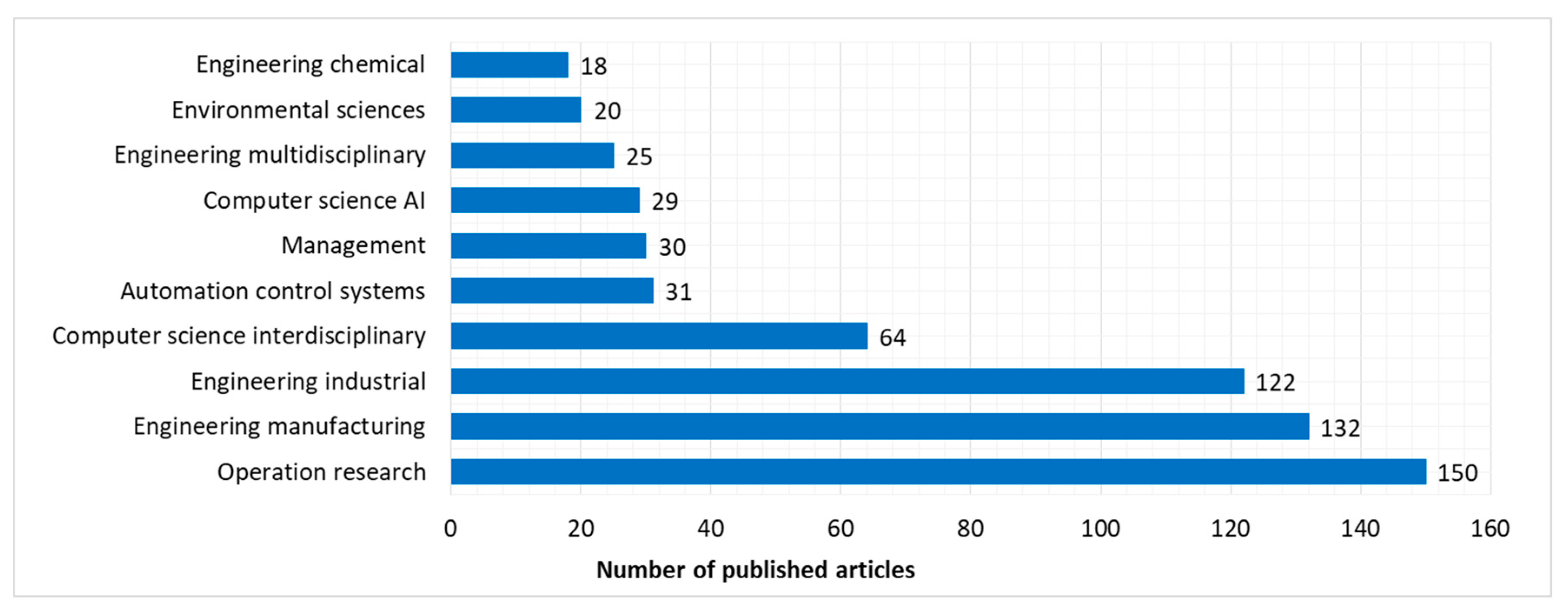
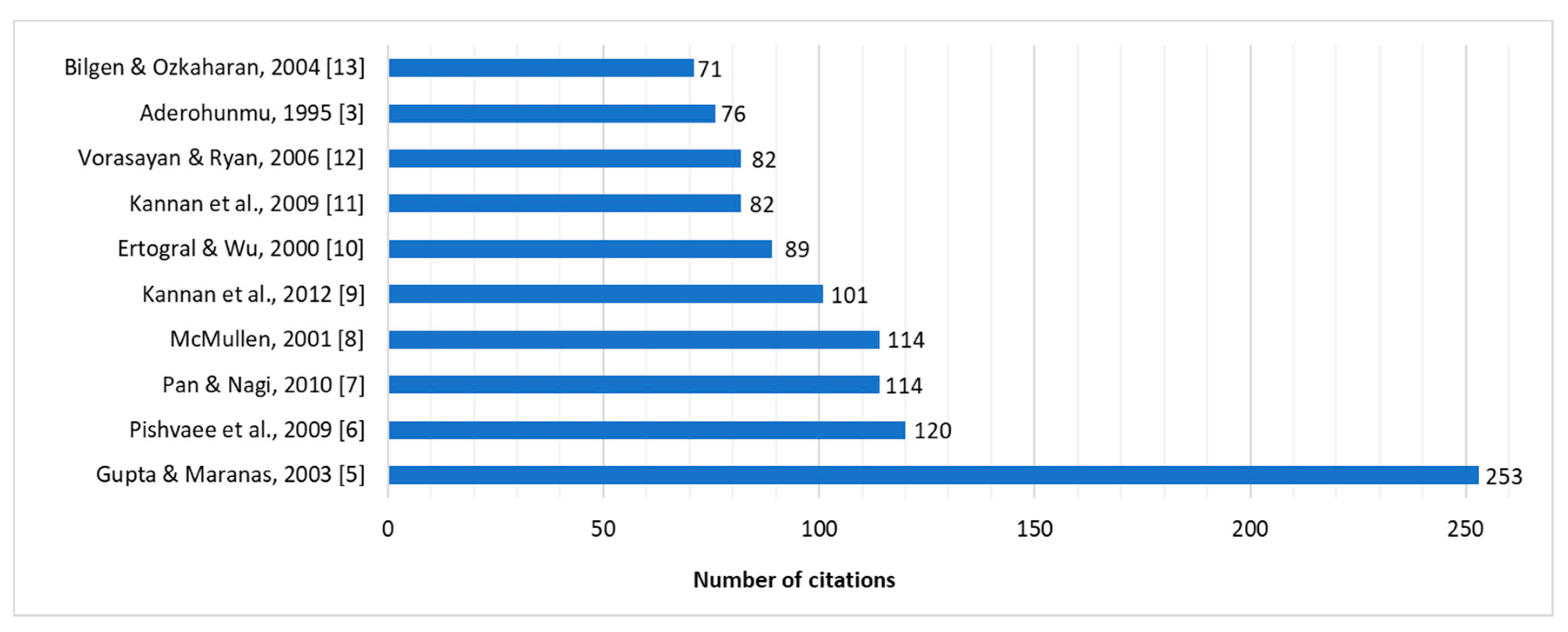
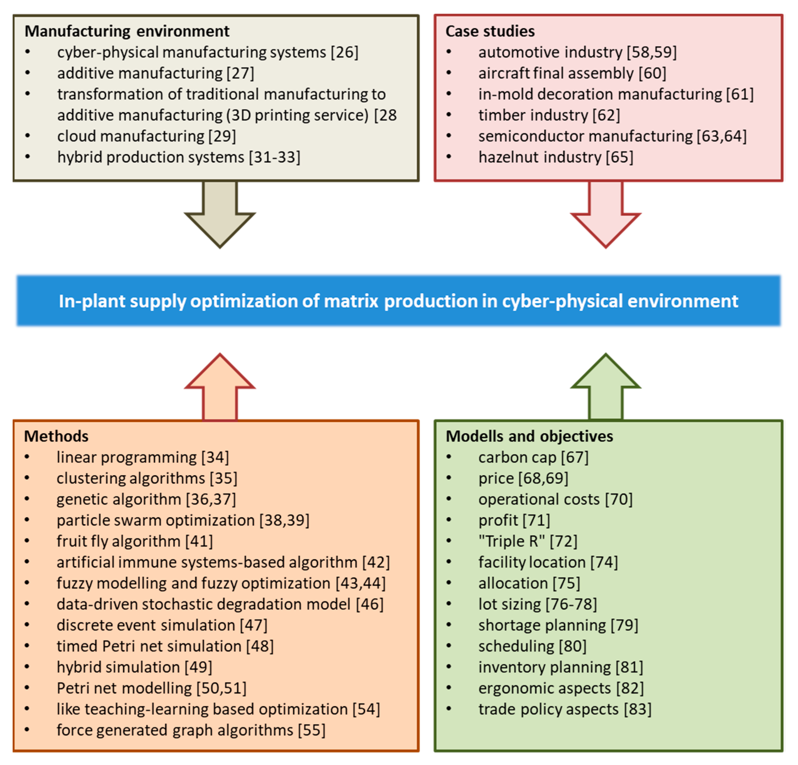
2.1. Descriptive Analysis

The reduced articles can be classified depending on the research area. Figure 1 shows the classification of these 370 articles considering ten subject areas. This classification shows that the majority are on engineering while operations research and computer sciences define the importance of computational methods related to the design of manufacturing related logistics systems.
As Figure 2 demonstrates, the optimization of manufacturing-related logistics systems has been researched in the past 20 years. The first articles in this field were published in 1995 focusing on just-in-time manufacturing [3] and process related simulation [4]. The number of published papers has been increased in the last five years; it shows the importance of this research field.
Articles were analyzed from a scientific impact point of view. The most usual form to evaluate articles from the scientific impact point of view is the citation. Figure 3 shows the ten most cited articles with their number of citations.
As Figure 4 demonstrates, most of the articles were published in journals with production and manufacturing topics, but a significant part of the papers was accepted for publication in journals focusing on computation, operation research, and expert systems. The distribution of journals shows that the design and operation problems of logistics systems in production and manufacturing are multidisciplinary problems, where not only technological but also environmental and other aspects must be taken into consideration.
We have analyzed the published articles from the Web of Science categories point of view. We have analyzed the distribution of articles in the following categories: operations research management science, engineering manufacturing, engineering industrial, computer science interdisciplinary, automation control systems, management, computer science artificial intelligence, engineering multidisciplinary, environmental sciences, engineering chemical, engineering electrical electronic, engineering environmental, green sustainable science, computer science software engineering, engineering mechanical, and mathematics interdisciplinary. The distribution of the categories is depicted in Figure 5. As the categories show, the design of manufacturing related logistics systems is based on optimization methods, and not only cost efficiency but also environmental and technological aspects are important, while automation and the application of smart solutions gain a more prominent role.
In the following step, the 370 articles were reduced after reading them. We excluded articles whose topic did not fit our interest and couldn’t address the optimization of manufacturing related logistics systems focusing on in-plant supply. After this reduction, we had 80 articles.

2.2. Content Analysis

In the 80s and 90s the so-called CIM addressed the first attempts to define hierarchy structured in smart factories [14]. CIM and FMS was the key topic [15], and things such as dynamic scheduling [16] and reactive MES [17] were invented then. After that, holonic manufacturing [18] and IMS was established.
A Holonic Manufacturing System (HMS) is a manufacturing system where key elements, such as machines, cells, factories, parts, products, operators, teams, etc., are modeled as ‘holons’ having autonomous and cooperative properties. The decentralized information structure, the distributed decision-making authority, the integration of physical and informational aspects, and the cooperative relationship among holons, make the HMS a new paradigm, with great potential for meeting today’s agile manufacturing challenges.
[19]
Information management was a challenge in a virtual enterprise environment characterised by distribution, autonomy and co-operation. Distributed information management architecture was one of the key topics for production planning and control. It provided not only basic services but also advanced services, like notification, security control, subscription, and data sending [20].
Some of the proposed models and concepts are missed, but the ideas still were appointed in sources, for example focusing on the optimization of the accuracy of the wire electro-discharge machining process [21] or the manufacturing of five-axis high speed milling of complex parts [22].
The smart factory is the integration of all recent IoT technological advances in computer networks, data integration, and analytics to bring transparency to all manufacturing factories. The Internet of Everything (IoE) is a concept that extends the Internet of Things (IoT) emphasis on machine-to-machine (M2M) communications to describe a more complex system that also encompasses people and processes. The steps to creating a smart factory are the followings [23]:
  • data transmission: get data to communicate from robot to machine to person,
  • connection: get this data to a large capacity IoT server,
  • big data processing: make the data visible and actionable to people for analysis.
Several new edge computing devices were launched recently. In Japan there is a general movement about first using common sense and later technology. Special processes are those in which more CPS (cyber-physical systems) are in use because models are closely related to machine controls. In EDM and other works about lasers, welding, etc., CPS are spreading. For instance, EDM edge computing is becoming a leading research line [24]. 5G and IoT will be key to enhancing and enabling the advances in manufacturing. 5G networks offer manufacturers and telecom operators the chance to build smart factories and truly take advantage of technologies such as automation, artificial intelligence, augmented reality for troubleshooting, and the Internet of Things [25].
The research in the field of manufacturing processes indicated a huge number of articles reporting the results of research projects in all fields of engineering and economic sciences. These researches are discussing a wide range of manufacturing solutions, from traditional manufacturing to cyber-physical manufacturing systems [26]. The improvement of 3D printing led to the appearance of a new decision to be made by production companies: how to make components for final products? Products can be produced either with traditional technology or with additive manufacturing. Additive manufacturing has a great impact on related supply chain and logistics solutions; therefore, it is important to put more and more effort into the research of additive manufacturing solutions [27]. Traditional routing, assignment and scheduling models and solutions must be transformed to cyber-physical models, like the transformation of conventional scheduling to 3D printing service scheduling demonstrates [28] in the case of cloud manufacturing, where distributed manufacturing resources are encapsulated into services and aggregated [29]. The additive manufacturing can lead to decentralized, flexible production facilities, where the customer’s demands can be produced with low financial risk; they are flexible and can respond rapidly to changes in demand [30]. In hybrid production systems, the manufacturing of new and remanufactured products is integrated. In hybrid production systems, special constraints caused by uncertainties in recycling processes must be taken into consideration [31,32,33].
The literature introduces a wide range of methods used to solve design problems of logistics processes in manufacturing, like integer programming, decision-making methods, heuristic and metaheuristic algorithms, Petri Net simulation, statistical approaches, simulation and simulation-based optimization, fuzzy modelling, and hybrid optimization approach. Linear programming, integer linear programming, and mixed integer linear programming can also be used for the optimization of logistics processes in manufacturing systems. Researchers developed a multi-objective mixed integer linear programming model to generate efficient solutions minimizing cost and assigning more reliable manufacturers in a dynamic manufacturing network [34]. Clustering algorithms, like K-mean, mean-shift, density-based spatial clustering, or agglomerative hierarchical clustering are widely used in the design of complex in-plant supply systems; they can be combined for multi-stage optimization with heuristic and metaheuristic algorithms. The combination of prioritized K-mean and genetic algorithm was used to optimize manufacturing related transportation processes [35]. Heuristic optimization methods are used in the case of NP-hard optimization problems: genetic algorithm was used to increase machine utilization, reduce throughput time and delivery delays [36,37], while discrete particle swarm optimization (PSO) was applied to solve the dynamic travelling salesman problem in chip manufacturing, where machine failure can force changes to the problem specification [38]. A typical application field of PSO is flow shop and job shop manufacturing [39] or the machine loading problem in flexible manufacturing systems, where the feeding process is generally robotized or automatized [40]. Heuristic methods can be used not only for the optimization of processes but also for the allocation of IT structure in the manufacturing process: a fruit fly algorithm was used to find the optimal location of the wireless sensor network in the intelligent workshop [41]. The in-plant supply of manufacturing processes is based on complex material handling systems, which were optimized with a hybrid multi-objective artificial immune systems-based algorithm [42]. Manufacturing processes are typical uncertain environments, where fuzzy modelling and fuzzy optimization offers suitable tools [43,44] and the fuzzy approach can easily integrate with other analytical or heuristic algorithms [45]. Researchers used an integrated data-driven stochastic degradation model to find the optimal maintenance strategy in chemical and manufacturing processes, where unit failures are caused due to equipment degradation [46]. Different types of simulation methods and tools can be used to optimize in-plant and external manufacturing related logistics processes, like discrete event simulation [47], timed Petri net simulation [48], and hybrid simulation integrating discrete and continuous time event simulation [49]. The Petri net modelling, the timed, colored, and fuzzy Petri net approaches are widely spread in the field of simulation of manufacturing related logistics systems [50,51]. Integrated approaches [52], multi-objective optimization problems [53] can be solved with other effective optimization methods, like teaching-learning based optimization [54], force generated graph algorithms [55], agent-based optimization methods [56], or TOPSIS [57]. Figure 6 shows the conceptual framework of the published articles demonstrating the new manufacturing environments, applied methods and tools, typical models, and case studies.
Several scenarios and case studies related to in-plant supply and material handling in manufacturing were assessed and evaluated to compare the effects of technology, logistics, human resources, and policies on the efficiency, reliability, and availability of value making. The case studies of manufacturing design are generally focusing on traditional manufacturing environment, and only a few of them are discussing the cyber-physical systems. The most important fields of case studies are from the automotive industry [58,59], but valuable case studies were published in the field of aircraft final assembly [60], in-mold decoration manufacturing [61], timber industry [62], semiconductor manufacturing [63,64], food manufacturing [65], and injection molding [66].
The objective functions and constraints of design and operation of in-plant supply systems of manufacturing processes include a wide range of economical, technical-technological, ecological, and logistic aspects. Green in-plant supply problems are represented by carbon cap constrained manufacturing system, where green solutions can support sustainability [67]. The financial aspects of manufacturing supply are analyzed from price [68,69], operational costs [70], and profit [71] points of view. Responsiveness, robustness, and resilience (known as “Triple R”) become more and more important in logistics and material handling [72] because customer satisfaction is based on “Triple R”-based performance of manufacturing and related logistics operations [73]. The objective functions and constraints are based on the problems of typical material handling related problems, like facility location [74], allocation [75], lot sizing [76,77,78], shortage planning [79], scheduling [80], inventory planning [81], and ergonomic [82] and trade policy aspects [83].

2.3. Consequences of Literature Review

More than 50% of the articles were published in the last four years. This result indicates the scientific potential of the design of in-plant supply solutions for manufacturing systems. The articles that addressed the optimization of in-plant supply and material handling solutions are focusing on a conventional manufacturing environment and only a few of them describe the design aspects of in-plant logistics solutions in cyber-physical environment. Therefore, this research topic still needs more attention and research. It was found that mathematical models and algorithms are important tools for the design and control of in-plant supply solutions since a wide range of models determines complex optimization problems. According to that, the main focus of this research is the modelling and optimization of in-plant supply focusing on extended and real-time logistics resource optimization from assignment, clustering, and scheduling points of view.
As a consequence, the main contributions of this article are the followings: (1) model framework of cyber-physical in-plant supply in matrix production; (2) mathematical description of in-plant supply of standardized, categorized manufacturing and assembly cells of the production matrix; (3) computational method to solve clustering, assignment, and scheduling of logistics resources; (4) computational results of the described model with various datasets and scenarios focusing on environmental impacts and reduction of GHG emission.

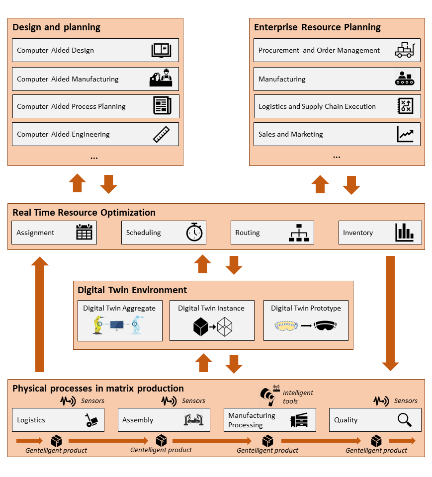
3. Methodology—Mathematical Modelling and Heuristic Optimization Method

As the KUKA matrix production paradigm defines, in-plant supply, and manufacturing processes are separated from each other, and the logistics system with variable accessories and tools of autonomous material handling and transportation machines (autonomous guided vehicles) is always able to supply all matrix cells [2]. Figure 7 demonstrates the model of a matrix production system focusing on real-time resource optimization.
The physical processes in matrix production include logistics (material handling, transportation and warehousing), assembly, manufacturing, processing and quality control. The physical process is transformed into a virtual system called digital twin, which can include digital aggregate, digital instance, and digital prototypes. The transformation is based on sensors, which collect data on resources, components, tools, and their environment. Machines, tools, products, and other logistics resources are connected with the digital twin through a sensor network. The extended and real-time optimization of supply-demands is supervised by the ERP, while forecasting and testing are performed in a digital twin environment.
In our in-plant supply chain model, there are two different types of deliveries to be performed. The first types are supply-demands, which are available from the ERP and they can be scheduled and assigned for a predefined time window. The second type of supply-demands must be scheduled and assigned in real-time which means that the scheduled routes must be changed so that the scheduled supply-demands will arrive within the time frame to the matrix cell. The in-plant supply model of matrix production includes m matrix cells (standardized production of assembly cells), α jobs and β time frame for scheduling of in-plant supply routes. The components and the tools are stored in specific stores (components warehouse and tool storage) and they are transported with AGV parking in an AGV-pool [2]. This in-plant supply model can be divided into two main parts: the first part is the extended scheduling based on ERP data, while the second part, the real-time scheduling, is based on information from the cyber-physical environment (intelligent tools, cooperative standardized assembly and manufacturing cells). The following decisions must be made: (a) clustering of available supply-demands; (b) routing and scheduling of clustered supply-demands; (c) rescheduling and rerouting of matrix cell’s supply in order to insert new supply-demands caused by malfunction of technology and logistics or caused by a new customer’s order to be fulfilled. The decision variable of the clustering problem is the assignment matrix which defines the assignment of supply-demands and supply routes. The decision variable of extended routing and scheduling problem is another assignment matrix, which defines the sequence of supply. In the case of the real-time rerouting and rescheduling, we also use an assignment matrix, in which some positions of sequences are changed to insert new supply-demand into the scheduled supply (Figure 8).
The methodology of our research includes the following main parts:
  • mathematical modelling of the cyber-physical matrix production system from an extended and real-time optimization point of view,
  • performance analysis of available heuristic solution algorithm and selection of the suitable algorithms,
  • application of suitable algorithms to solve the extended and real-time clustering, routing, and assignment problems,
  • validation of the model and the algorithm with scenario analysis.

3.1. Mathematical Modelling of Extended and Real-Time Resource Optimization in Cyber-Physical Matrix Production

Within the frame of this chapter, a two-level mathematical model is discussed including extended and real-time scheduling problems of in-plant supply of matrix production.

3.1.1. Extended Logistics Resource Optimization

The extended optimization of supply resources in matrix production can be divided into two main phases. The first phase is a clustering phase, where the available supply-demands are clustered based on time frame related objective function. The second phase represents a vehicle routing problem, where the clustered supply-demands are scheduled.

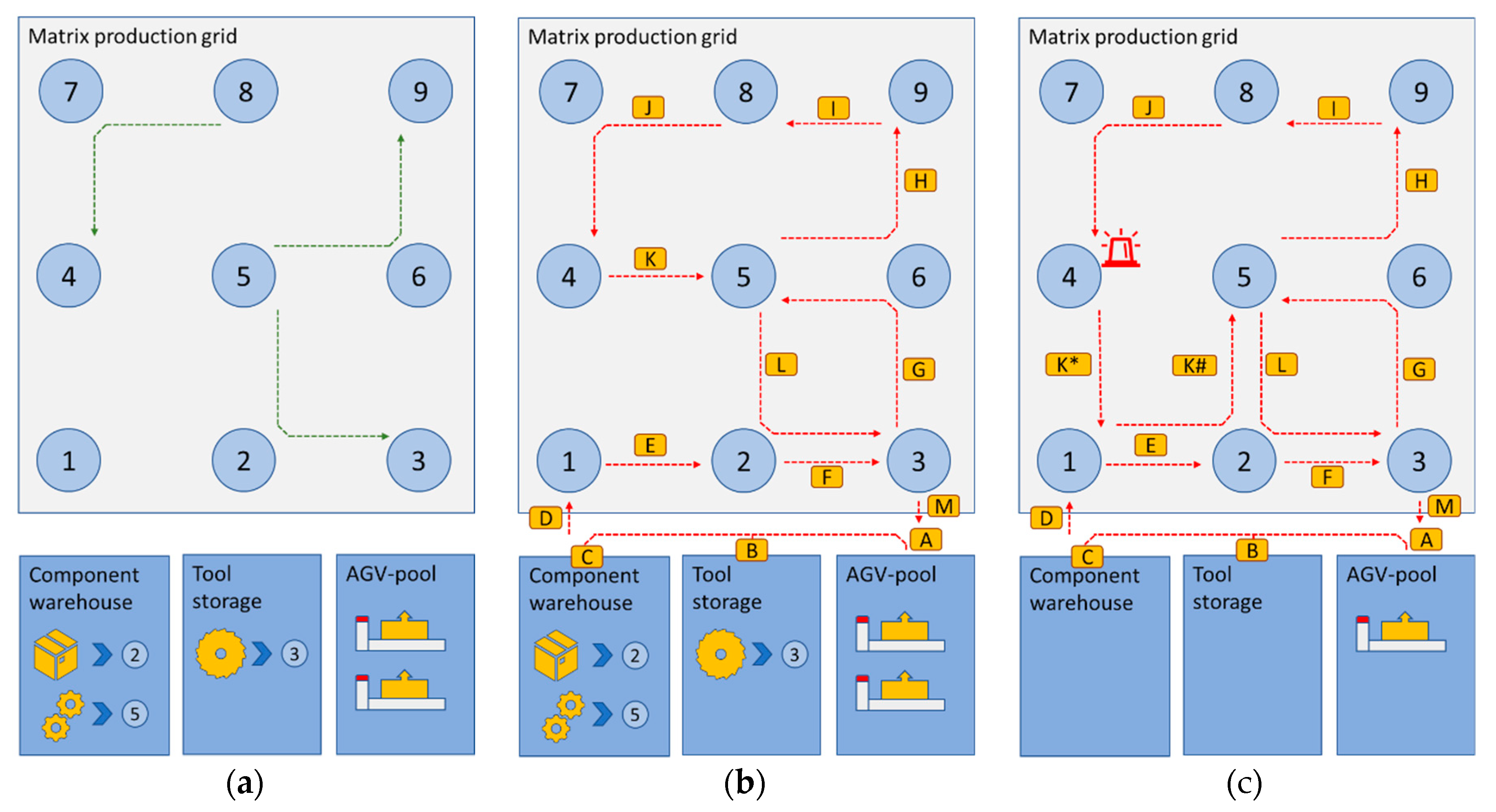
Clustering of Supply-Demand

The objective function of the clustering of supply-demands is the minimization of the total time deviance of supply-demands from the average time frame, which can be calculated as the sum of supply-demands assigned to route r in relations warehouse–matrix cell, tool storage–matrix cell and among matrix cells:
TD W T M = TD W + TD T + TD M m i n .
where TD W is the time deviance of clustered supply-demands from component warehouse to matrix cells, TD T is the time deviance of clustered supply-demands from tool storage to matrix cells, and TD M is the time deviance of clustered supply-demands among matrix cells.
The first part of the objective function includes the minimization of time frame deviance from the average time frame between the component warehouse and matrix cells:
TD W = r = 1 r m a x ( x i α β r W M t i α β W ¯ t r W ¯ )   and   t r W ¯ = i = 1 m α = 1 α m a x β = 1 β m a x x i α β r W M t i α β W ¯
where, t i α β W ¯ is average time frame of supply-demand from the component warehouse to matrix cell j for job α in time frame β , is the average time frame of route r, x i α β r W M is the assignment matrix of supply-demands from component warehouse to matrix cells. x i α β r W M takes value 1 if the supply-demand from component warehouse to the matrix cell i for job α in time frame β is assigned to route r, otherwise 0.
The second part of the objective function includes the minimization of time frame deviance from the average time frame between tool storage and matrix cells:
TD T = r = 1 r m a x ( x i α β r T M t i α β T ¯ t r T ¯ )   and   t r T ¯ = i = 1 m α = 1 α m a x β = 1 β m a x x i α β r T M t i α β T ¯
where, t i α β T ¯ is average time frame of supply-demand from the tool storage to matrix cell j for job α in time frame β , t r T ¯ is the average time frame of route r, x i α β r T M is the assignment matrix of supply-demands from component warehouse to matrix cells. x i α β r T M takes value 1 if the supply-demand from the tool storage to the matrix cell i for job α in time frame β is assigned to route r, otherwise 0.
The third part of the objective function includes the minimization of time frame deviance from the average time frame among matrix cells:
TD M = r = 1 r m a x ( x i j α β r M M t i j α β M M ¯ t r M M ¯ )   and   t r M M ¯ = i = 1 m j = 1 n α = 1 α m a x β = 1 β m a x x i j α β r M M t i j α β M M ¯
where t i j α β M M ¯ is average time frame of supply-demand between matrix cell i and matrix cell j for job α in time frame β , t r M M ¯ is the average time frame of route r, x i j α β r M M is the assignment matrix of supply-demands between matrix cell i and matrix cell j for job α in time frame β . x i j α β r M M takes value 1 if the supply-demand from matrix cell i to matrix cell j for job α in time frame β is assigned to route r, otherwise 0.
The solutions of the above-described clustering problem are limited by the following two constraints related to time frame and capacity of AGVs:
Constraint 1: We can define an upper limit for time frame deviance for each route and it is not permitted to exceed the upper limit of time frame deviance within route r:
  i , α , β , r :   max i α β r | t i α β W ¯ t r W ¯ | t W m a x
  i , α , β , r : max i α β r | t i α β T ¯ t r T ¯ | t T m a x
  i , j , α , β , r : max i j α β r | t i j α β M M ¯ t r M M ¯ | t M M m a x
where t W m a x is the upper limit of time frame deviance for supply-demands from component warehouse to matrix cells, t T m a x is the upper limit of time frame deviance for supply-demands from tool storage to matrix cells, and t M M m a x is the upper limit of time frame deviance for supply-demands among matrix cells.
Constraint 2: We can define the upper limit of AGVs’ loading capacity and it is not permitted to exceed this upper limit after assigning suitable supply-demands from component warehouse to matrix cells, from tool storage to matrix cells and among matrix cells:
  r : i = 1 m α = 1 α m a x β = 1 β m a x ( x i α β r W M q i α β W M + x i α β r T M q i α β T M ) + i = 1 m j = 1 n α = 1 α m a x β = 1 β m a x x i j α β r M M q i j α β M M C r m a x
where q i α β W M amount of required component from the component warehouse to the matrix cell i for job α in time frame β , q i α β T M amount of required component from the tool storage to the matrix cell i for job α in time frame β , q i j α β M M amount of required component from matrix cell i to the matrix cell j for job α in time frame β , and C r m a x is the upper limit of loading capacity of AGV in route r.

Routing and Scheduling of Supply-Demand

The objective function of the routing and scheduling of supply-demands is the minimization of energy consumption:
  r , β :     λ = 2 λ m a x ξ s r λ 1 s r λ ( p s r λ 1 x , p s r λ 1 y , p s r λ x , p s r λ y ) e r m i n .
where λ m a x is the number of supply-demands assigned to route r, s r λ is the ID of supply-demand assigned as destination λ to route r, p i x and p i y are the x and y coordinates of matrix cell i, and ξ s r λ 1 s r λ it the length of the route between matrix cell λ 1 and matrix cell λ in route r and e r is the specific energy consumption of AGV used in route r.
The solutions of the above-described routing and scheduling problem are limited by the constraints related to the time frame of arrival times to matrix cells.
Constraint 3: Depending on the velocity of the AGVs we can calculate the travelling time among matrix cells, component warehouse or tool storage and the arrival time can be defined. It is not permitted to exceed the upper and lower limit of time frame for each supply-demand to the matrix cells:
  r , λ :           t r λ m i n λ = 2 λ m a x ξ s r λ 1 s r λ ( p s r λ 1 x , p s r λ 1 y , p s r λ x , p s r λ y ) v r ¯ t r λ m a x
where t r λ m i n and t r λ m a x is the lower and upper limit of the arrival time to the matrix cell assigned as node λ to the route r and t r λ m i n = t s r λ α β m i n and t r λ m a x = t s r λ α β m a x
To simplify the representation of different types of supply-demands, we integrate the component warehouse–matrix cells, tool storage–matrix cells, and matrix cell–matrix cell relations into one type of relation and we create a virtual supply-demand matrix as follows:
  • Matrix cell–matrix cell relations are simply added to the virtual demand matrix:
    q i j α β = q i j α β M M
  • Component warehouse–matrix cell relation is transformed into a matrix cell–matrix cell relation. The component amount will be added as initial loading to the AGVs loading and a virtual matrix cell–matrix cell relation is added to the virtual supply-demand matrix:
    q i i α β = q i α β W M
  • Tool storage–matrix cell relation is transformed into a matrix cell–matrix cell relation. The tool amount will be added as initial loading to the AGVs loading and a virtual matrix cell–matrix cell relation is added to the virtual supply-demand matrix:
    q i i α β = q i α β T M
In the same way, we can create the virtual time frame matrix and assignment matrix:
x i i α β r = x i α β r T M       x i i α β r = x i α β r W M      x i j α β r = x i α β r M M
t i i α β r = t i α β r T M t i i α β r = t i α β r W M   t i j α β r = t i α β r M M
As an example, Figure 9 demonstrates the transformation of assignment matrices to a virtual assignment matrix.
Using the virtual assignment, supply-demand and time frame matrices the objective function can be simplified as follows:
TD W T M = r = 1 r m a x ( x i j α β r t i j α β ¯ i = 1 m j = 1 n α = 1 α m a x β = 1 β m a x x i j α β r t i j α β ¯ )
while Constraints 1 (5)–(7) can be written as:
  i , j , α , β , r :   max i j α β r | t i j α β ¯ t r ¯ | t m a x
and Constraints 2 (8) can be written as:
  r :           q 0 r + i = 1 m j = 1 n α = 1 α m a x β = 1 β m a x x i j α β r q i j α β C r m a x
where q 0 r is the initial loading of AGV r that can be calculated as follows:
  r :           q 0 r = i = 1 m j = 1 n α = 1 α m a x β = 1 β m a x ( x i j α β r W M + x i j α β r T M )
The described mathematical representation of the extended logistics resource optimization makes it possible to optimize the in-plant supply of manufacturing and assembly cells of matrix production in a cyber-physical system. This extended optimization is possible if the supply-demand of the manufacturing and assembly cells of the matrix production is known for a predefined time window represented by β in the model.
The next phase of the optimization is the real-time rerouting and rescheduling of routed AGVs and supply tours caused by new orders, or malfunction of technological, logistic, or human resources.

3.1.2. Real-Time Logistics Resource Optimization

The second phase of our approach includes a real-time routing and scheduling problem. Within the frame of this phase, the extended assignment and routing can be modified depending on the real-time information of matrix production systems and ERP.
The decision variables of the real-time logistics resource optimization describe the decisions to be made. In this model it must be decided which new supply-demand by which AGV in which time is picked up. This decision represents an integrated assignment and scheduling problem. With this in mind, we define the following positions based on the results of extended logistics resource optimization describing the layout of the matrix production supply problem:
  • p s r λ x , p s r λ y is the x and y coordinate of the scheduled matrix cell s r λ of scheduled route r,
  • p ψ P x and p ψ P y is the x and y coordinate of the pickup matrix cell of the new supply-demand ψ ,
  • p ψ D x and p ψ D y is the x and y coordinate of the destination matrix cell of the new supply-demand ψ .
The objective function of the problem describes the minimization of the energy consumption of the whole in-plant supply process including scheduled routes (extended optimization) and new supply-demands (real-time optimization).
E C = E C S R + E C N S P + E C N S D min .
where E C S R is the energy consumption of scheduled supply-demands without any assigned new supply-demands, E C N S P is the energy consumption of pickup route of new assigned and scheduled supply-demand, and E C N S D is the energy consumption of delivery route of new assigned and scheduled supply-demand.
The first part of the objective function (20) includes the sum of energy consumption of scheduled supply-demands without assignment of new supply-demands, where the energy consumption is the function of positions of matrix cells for pickup and delivery, the loading of AGVs and the specific energy consumption, as written in (9).
The second part of the objective function (20) includes the energy consumption of the pickup route of new assigned and scheduled supply-demand:
E C N S P = r = 1 r m a x ψ = 1 ψ m a x x r λ ψ P ( ξ s r λ 1 ψ ( p s r λ 1 x , p s r λ 1 y , p ψ x , p ψ y ) + ξ s r λ ψ ( p s r λ x , p s r λ y , p ψ x , p ψ y ) ) e r
where r m a x is the total number of scheduled routes within the time frame, ψ m a x is the number of new supply-demands within the time frame (in the case of real-time scheduling ψ m a x = 1 because new supply-demands are scheduled real-time and they are not collected to be scheduled together), x r λ ψ P is the assignment matrix of pickup matrix cells of new supply-demands to the scheduled routes. x r λ ψ P takes value 1 if the new supply-demand ψ is assigned to route r following scheduled supply-demand λ , otherwise 0.
The third part of the objective function (20) includes the energy consumption of the delivery route of new assigned and scheduled supply-demand:
E C N S D = r = 1 r m a x ψ = 1 ψ m a x x r λ ψ D ( ξ s r λ 1 ψ ( p s r λ 1 x , p s r λ 1 y , p ψ x , p ψ y ) + ξ s r λ ψ ( p s r λ x , p s r λ y , p ψ x , p ψ y ) ) e r
where x r λ ψ D is the assignment matrix of destination matrix cells of new supply-demands to the scheduled routes. x r λ ψ D takes value 1 if the pickup matrix cell of the new supply-demand ψ is assigned to route r following scheduled supply-demand λ , otherwise 0.
The solutions of this integrated assignment and scheduling problem are limited by the following three constraints:
Constraint 4: The capacity of AGV is not to exceed after assignment of new supply-demand. The new loading of AGV r passing pickup matrix cell λ 1 can be calculated by adding the assigned new supply-demand and subtracting the value of a previously assigned delivery of an open task as follows:
  r , λ , β : q 0 r + b = 3 λ α = 1 α m a x β = 1 β m a x q s r b 2 s r b 1 α β + q ψ N S + b = λ + 1 λ m a x α = 1 α m a x β = 1 β m a x q s r b 1 s r b α β C r m a x
Constraint 5: It is not permitted to exceed the upper and lower limit of pickup time frame for each scheduled matrix cell.
  r , λ :           t r λ P m i n t r λ ψ P 1 + t r λ ψ P 2 + t r λ ψ P 3 + t r λ ψ P 4 t r λ P m a x ,
where
t r λ ψ P 1 = t 0 r + b = 3 λ ξ s r b 2 s r b 1 ( p s r b 2 x , p s r b 2 y , p s r b 1 x , p s r b 1 y ) v r ¯ ,
t r λ ψ P 2 = ξ s r λ 1 ψ ( p s r λ 1 x , p s r λ 2 y , p s r ψ x , p s r ψ y ) v r ¯   and   t r λ ψ P 3 = ξ ψ s r λ ( p s r λ x , p s r λ y , p s r ψ x , p s r ψ y ) v r ¯
t r λ ψ P 4 = t 0 r + b = λ + 1 λ m a x ξ s r b 1 s r b ( p s r b 1 x , p s r b 1 y , p s r b x , p s r b y ) v r ¯ ,
where t r λ P m i n and t r λ P m a x is the lower and upper limit of pickup time for matrix cell s r λ , t r λ ψ P 1 is the travelling time from the AGV-pool to the predecessor matrix cell of the new supply-demand’s matrix cell ψ in route r, t 0 r is the initial travelling time from the AGV-pool to the first scheduled matrix cell, t r λ ψ P 2 is the travelling time from the predecessor matrix cell to the new supply-demand’s matrix cell ψ in route r, t r λ ψ P 3 is the travelling time from the new supply-demand’s matrix cell ψ to the following matrix cell in route r, and t r λ ψ P 4 is the travelling time from the pickup matrix cell of the new supply-demand ψ to matrix cell λ in route r.
Constraint 6: It is not permitted to exceed the upper and lower limit of delivery time frame for each scheduled matrix cell.
  r , λ :           t r λ D m i n t r λ ψ D 1 + t r λ ψ D 2 + t r λ ψ D 3 + t r λ ψ D 4 t r λ D m a x ,
where t r λ ψ D 1 , t r λ ψ D 2 , t r λ ψ D 3 , and t r λ ψ D 4 can be calculated in the same was as in (25)–(27).
Constraint 7: It is not permittFed to exceed the upper and lower limit of pickup and delivery time frame for each new supply-demand.
  ψ :           t ψ P N m i n t r λ ψ P 1 + t r λ ψ P 2 t ψ P N m a x          t ψ D N m i n t r λ ψ D 1 + t r λ ψ D 2 t ψ D N m a x ,
where t ψ P N m i n and t ψ P N m a x is the lower and upper limit of pickup time for new supply-demand ψ and t ψ D N m i n and t ψ D N m a x is the lower and upper limit of pickup time for new supply-demand ψ .
The decision variables have two different types: the decision variables of the assignment problems are integer matrices, while the decision variables of the scheduling problem are matrices with real values. The assignment matrices x i j α β r , x r λ ψ P and x r λ ψ D define the scheduling of supply-demands both in extended and real-time optimization, so we have only integer decision variables.
Figure 10 demonstrates the model framework including time frame and capacity constraints. As the figure shows, the assigned new supply-demands have a great impact on the performance of supply routes.
However, without constraints of time frame and capacity the new supply-demand can be assigned to the nearest matrix cells, but in the case of time and capacity related constraints the assignment and scheduling is an NP-hard optimization problem, therefore we suggest a heuristic approach to solve it.

3.2. Heuristic Optimization for Extended and Real-Time Logistics Resource Optimization Based on Black Hole Algorithm

Within the frame of this part of the article, a multiphase optimization algorithm is described. The algorithm includes an extended and real-time optimization phase. Within the extended phase, the in-plant supply of known supply-demands of the matrix production system is optimized. This extended optimization includes the clustering of supply-demands, the routing and the scheduling of clustered supply-demands. The second phase of the optimization is the real-time rerouting and rescheduling, where the existing routes are redesigned in order to insert new supply-demands into the existing routes. The objective function of the optimization algorithm includes time-related aspects, while time-frames and capacities are taken into consideration. The algorithm makes it possible to analyze the solutions from a sustainability point of view because greenhouse gas emission can be calculated. Within the frame of performance analysis, various heuristic algorithms are tested to measure their efficiency. Table 1 shows the results of this performance analysis.
As the performance analysis shows, the results of black hole and flower pollination algorithms are comparable with genetic and harmony search algorithms.

3.2.1. Black Hole Optimization-Based Clustering

There is a wide range of clustering algorithms in the literature, which is suitable for the solution of clustering problems without complex restrictions. K-means clustering, mean-shift clustering, density-based spatial clustering, and agglomerative hierarchical clustering algorithms belong to the most well-known general clustering algorithms. However, their implementation codes are quite simple, but they have disadvantages:
  • K-mean: the classes must be defined [84];
  • Mean-shift: the size of the sliding window must be defined [85];
  • Density-based spatial clustering: its performance is low in the case of varying density of points [86];
  • Agglomerative hierarchical clustering: its complexity is O ( n 3 ) while K-means is linear [87].
The constraints and the complexity of the multi-dimensional search space make the clustering problem NP-hard, which means that heuristic clustering methods are suitable to solve the clustering problem of the extended logistics resource optimization in matrix production.
The idea of black holes was first suggested by John Michel and Pierre-Simon Laplace. They proposed the existence of “invisible stars”. They calculated its mass and size, which is the so-called event horizon in today’s science. Later, in 1916 Albert Einstein predicted the existence of black holes with his general relativity theory. The first black hole called Cygnus X-1 was recognized by John Wheeler in 1971. Black holes are strange and fascinating places in space where the gravitation forces are so high that they can trap not only particles, planets, and stars but also light. Black holes are born when stars die. There are three types of black holes depending on their size and weight: supermassive black holes, stellar black holes, and miniature black holes. The black hole optimization is based on this phenomenon of black holes. Black holes have four layers: space outside the photonsphere, space between photonsphere and event horizon, space inside the event horizon, and the singularity, where the mass of the black hole in concentrated in one single point. The photon sphere is a spherical region of non-spinning black holes; photons reaching the photon sphere are not captured but they are forced to travel in orbits. The distance between particles and the black hole has a great impact on the behavior of the particles. If the distance between a particle is much higher than the Schwarzschild radius, then the particle can move in any direction. If this distance is larger than the Schwarzschild radius, but this difference is not too much, the space-time is deformed, and more particles are moving towards the center of the black hole than in other directions (Figure 11).
The event horizon and the photon sphere can be calculated as follows:
r e h = 2 g M c 2 ,   and   r p s = 3 2 r s
where g is Newton’s gravitational constant, M is the mass, and c is the speed of light.
Black hole algorithm belongs to the swarm intelligence algorithm, which are inspired either by living bodies, like ants [88], bees [89], fishes [90], bats [91], krill herds [92], fireflies [93], fruit flies [94], bacteria’s [95], or by other natural phenomena, like gravitation [96], big-bang [97], or intelligent water drop [98]. Black hole optimization is used in a wide range of NP-hard optimization problems, like investigating the critical slip surface of soil slope [99], solving the non-unicost set covering problem [100], optimization of consignment-store-based supply chain [101], thermodynamic optimization of a Penrose process [102], power flow optimization [103], and design of electromagnetic devices [104], but one of its most important application fields is the clustering. The black hole algorithms have six phases as follows:
  • big-bang phase: this phase is the initialization of the position and velocity of stars in the multidimensional search space. The stars represent potential solutions of the optimization problem, where the coordinates of the stars in the search space are the values of the decision variables. Stars can be initialized only inside the search space.
    p i = ( p i , 1 , p i , 2 p i , n ) [ p i , j m i n p i , j m a x ]
  • evaluation phase: this phase includes the calculation of the objective function based on the parameters represented by the coordinates of the star.
    v i = f ( p i , 1 , p i , 2 p i , n )
  • selection of black hole: within the frame of this phase a new black hole is defined as having the highest value of objective function. This star has the highest weight (represented by the value of objective function) and therefore it has the highest force of gravity and it is the center of movement of stars in the next movement phase.
    p ¯ B H = p ¯ i v B H = max i ( v i )
  • moving of stars: in this phase of the algorithm, a new position of stars is calculated. The movement of the stars can be influenced only by the black hole, but it is also possible to take into consideration the gravity force of the other stars.
    p i , j ( t + Δ t ) = p i , j ( t ) + R n d | p B H ( t ) p i , j ( t ) |
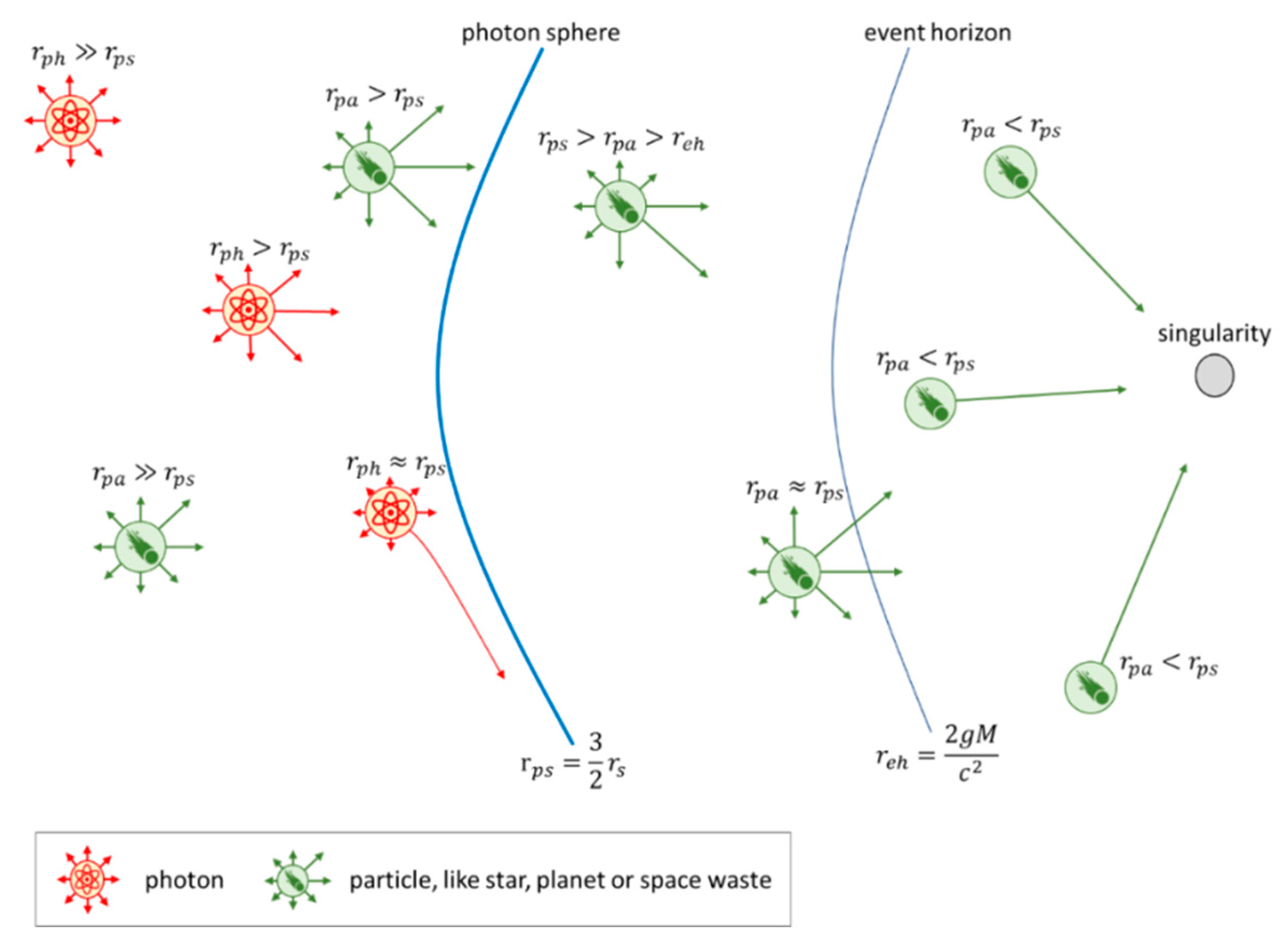
  • decreasing the event horizon and the photon sphere: in this phase, the size of the event horizon and the photon sphere is decreased based on the Hawking radiation, which describes the lost weight process of black holes. This phase makes it possible to prevent the absorption of stars representing solutions of the optimization problem near the optimum:
    r e h = v B H ϖ · i = 1 m v i   and   r p s = 3 2 v B H ϖ · i = 1 m v i ,
    where ϖ is the number of the current iteration step.
  • shift the position of the black hole: in this phase of the optimization we use the idea of Hawking radiation. Particles can escape and the black hole’s mass reduces because if a particle–antiparticle pair is created beyond the event horizon, it is possible to have one drawn into the black hole itself while the other is ejected [105]. The position of the black hole is shifted using the following calculation:
    P ¯ B H ( t + Δ t ) = p B H ( t + Δ t ) + v B H ϖ · μ · i = 1 m v i
    where μ is the shift-factor.
We demonstrate the clustering with a short example shown in Table 2 and Table 3. Table 2 shows the parameters of the clustering problem. There are 12 tasks which must be clustered within a predefined time frame so that the objective function is the minimization of time deviance of average supply time (1), while time and capacity related constraints (5)–(8) must be taken into consideration. As Table 2 shows, the loadings to be supplied are given in loading units.
The algorithm clustered the dataset given in Table 2 and resulted a time deviance of 104 min, while the constrained loading capacity of AGVs was not exceeded. Within the frame of the extended optimization of logistics resources of matrix production, we are using the above-mentioned black hole optimization-based clustering algorithm to find the best sets of supply-demands to be assigned to supply routes in order to minimize the time deviance from the time frames. As Table 3 shows, in this simple scenario, two supply routes must be performed to minimize the objective function while the upper limit of available AGVs is not exceeded.

3.2.2. Discretized Flower Pollination-Based Routing and Scheduling for Extended and Real-Time Optimization

Flower pollination algorithm is used in many fields of science: maximizing area coverage in wireless sensor networks [106], sizing optimization of truss structures [107], economic dispatch problems in modern power systems [108], optimizing wire electrical discharge machining [109], or calculation of maximum permitted capacity of photovoltaic in distribution network [110].
The flower pollination algorithm takes its metaphor from nature, from the pollination process of plants. Pollination is the act of transferring pollen grains from the male anther of a flower to the female stigma. External agents are responsible for the transportation of pollen grains. Typical agents are the following: insects, wind, birds, mammals, or water. Floral pollination algorithms are based on this natural phenomenon and their most important rules are the followings: [111]: the potential solutions of the optimization problem are represented by pollen grains; the global search in the search space is modelled through the biotic pollination; the local search in the search space is modelled by abiotic pollination and self-pollination; the global and local search is controlled through a switching probability between biotic, abiotic, and self-pollution. The algorithm has the following phases:
  • initialization of parameters: in this phase both problem-specific and algorithm-specific parameters are initialized. Problem-specific parameters are the parameters of search space (dimensions and size) and the constraints-defined parameters. Algorithm-specific parameters are the following: switch parameter between local and global search, distribution function parameters for Lévy flight, termination criteria, and the number of pollen grains.
  • calculation of the initial solutions: in this phase, the initial potential solutions of the optimization problem are defined.
  • evaluation of pollen grains: within the frame of this phase, pollen grains are evaluated based on the objective function of the optimization problem.
  • initialization of iteration phase: in this phase, a random number h [ 0 , 1 ] is generated to switch between global and local search option. If h h then global pollination (biotic pollination) takes place otherwise local pollination (abiotic pollination) takes place.
  • biotic pollination phase: this phase represents the global search in the search space. The operator is based on Lévy flight and can be defined as follows:
    ω i t + 1 = ω i t + L ( λ ) ( ω i b e s t , t ω i t )
    where ω i t is the value of variable i at iteration step t, ω i b e s t , t is the value of variable i at iteration step t in the case of the global best solution and L ( λ ) is the Levy distribution.
  • abiotic pollination: this phase represents a local search, in which pollen grains are spread to a local neighbor:
    ω i t + 1 = ω i t + ψ ( ω ϑ t ω ζ t ) ,    ω i ζ i
    where ω ϑ t and ω ι ζ t are random selected pollen grains about the neighborhood of the currently processed pollen grain and ψ [ 0 , 1 ] is a random number.
  • transformation of the continuous representation into permutation-based representation: within the frame of this phase the continuous variables are transformed into discrete numbers describing a permutation-based problem. We are using the smallest position value rule and the largest order value rule [112] for this transformation (Table 4).
  • checking the termination criteria: in this phase, the following termination criteria’s can be checked: computational time, iteration steps, the value of the best solution, lower limit of convergence speed.
Within the frame of the remaining part of this chapter, we will demonstrate the performance of the above-mentioned hybrid heuristic optimization method including clustering, assignment, and scheduling problems. In this scenario, 36 assembly stations are in around and there are 12 supply-demands to be clustered, routed, and scheduled. Table 5 shows the input parameters of the scenario, while Table 6 demonstrates the optimal clustering of the 12 supply-demands.
The upper limit of loading capacity of the AGVs is 38 and the clustering algorithm has found the best clusters for extended scheduling and routing with a maximum capacity of 34 and 35 LUs.
Figure 12 demonstrates the solution of extended clustering and routing problems including two routes. The value of the objective function is 137 min, while the total length of the unloaded sections is 3468 m.
Increasing the available loading capacity of AGVs the extended clustering and routing gives a better solution (Figure 13), because the time frame deviance is only 104 min.
If the objective function of the extended clustering and routing problem is the minimization of the empty routes, then the energy efficiency can be minimized, but the time frame deviance is too high and some supply-demands cannot be performed within the lower and upper limit of the predefined time frame. The minimization of the length of empty routes can be performed in the case of one route, which means that the available loading capacity of AGV must be higher than in the case of scenarios 1 and 2. In the case of scenario three, the total length of the empty routes is 2948.7 m, while the required AGV’s capacity is 69 LU and the total time frame deviance is 192 min. The key functionality of the algorithm has been explained. Figure 14 and Figure 15 show the pseudocode of the algorithm because the details of the software engineering part would be interesting for anyone aiming to replicate the implementation.

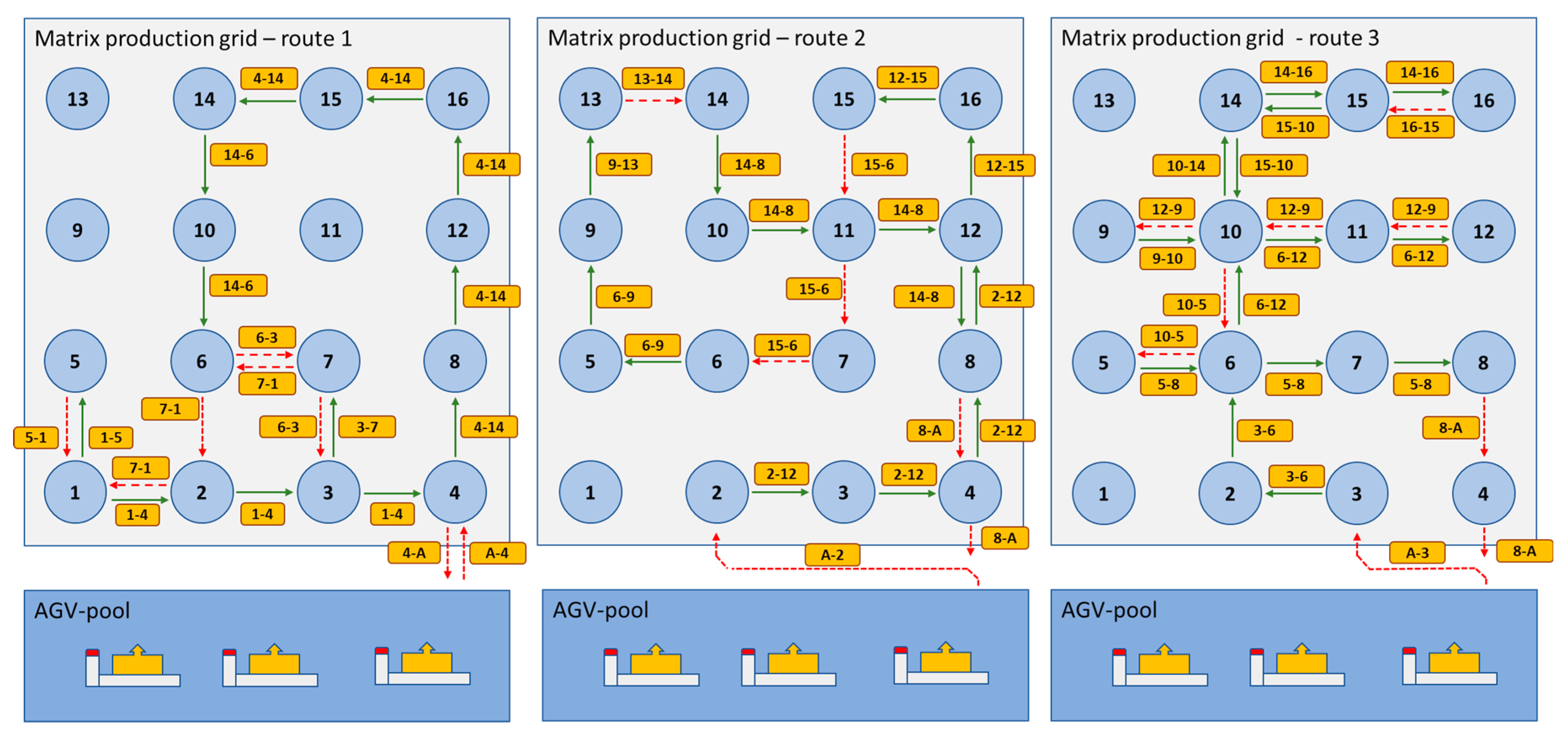
4. Results from the Scenario Analysis of Extended and Real-Time Logistics Resource Optimization in Matrix Production

Within the frame of this chapter, a scenario analysis demonstrates the application possibilities of the above described mathematical model and validates the applied heuristic optimization algorithm. The scenario is simplified to make examples as perspicuous as possible. We have chosen a simple scenario, which makes it possible to check the performance of the optimization algorithm and to validate the suggested model and solution algorithm. It makes sense to consider this specific scenario because both the clustering and the routing/rerouting problems can be demonstrated. In this scenario, 16 assembly stations are in a matrix grid and there are 16 supply-demands to be clustered, routed and scheduled. Table 7 shows the input parameters of the scenario, while Table 8 demonstrates the optimal clustering of the 16 supply-demands.
The upper limit of loading capacity of the AGVs is 120 and the clustering algorithm has found the best clusters for extended scheduling and routing with a maximum capacity of 109, 79, and 113 LUs.
Figure 16 demonstrates the solution of extended clustering and routing problem including three routes. The value of the objective function (total deviance of time frame) is 205.67 min, while the total length of unloaded sections is 372 m. The length of loaded routes is 444 m and the total length of the three supply routes is 816 m. The maximum loading of AGVs is 109, 79, and 113 LU, which means a capacity utilization of 91%, 66%, and 94%.
The next phase of the optimization is the real-time scheduling. Within the frame of our scenario, one supply-demand must be performed. The optimization algorithm is responsible for the reclustering, rerouting, and rescheduling of the routes in order to find the most energy efficient way, while time frame and capacity related constraints are taken into consideration. The new supply-demand must be performed between matrix cell 2 and 12, the time frame to perform this supply chain is between 10:30 and 10:45 and the loading is 21 LU. The results of reclustering are shown in Table 9 and Figure 17.
The value of the objective function (total deviance of time frame) is 237.75 min, while the total length of unloaded sections is 372 m. The length of loaded routes is 492 m and the total length of the three supply routes is 864 m. The maximum loading of AGVs is 114, 91, and 117 LU, which means a capacity utilization of 95%, 76%, and 98%.
The AGVs are using electricity. As the comparison of the World Nuclear Association shows, the greenhouse gas (GHG) emission depends on the electricity generation source (Figure 18).
Using the specific emission in g/liter fuel consumption and calculate the proportion of them to the GHG emission reported by World Nuclear Association [113] we can calculate the specific virtual emission of used electricity (Table 10).
However, energy consumption of AGVs depends on both the length of routes and loading of AGVs, but within the frame of our model, we calculate with an average loading. As previous research results highlight, energy consumption minimization is regarded as the optimal object to planning efficient routes for heterogeneous AGVs. The energy consumption of electric AGVs is between 40 and 150 Wh/km depending on the loading weight [115].
Table 11, Table 12 and Table 13 shows the calculated virtual GHG emission in the case of lignite, oil, and photovoltaic based electricity generation.
The above-described scenario validated the presented model based on extended and real-time routing, scheduling, and assignment and justifies the fact that in matrix production the enhanced logistics performance must be optimized in order to increase energy efficiency and decrease GHG emission. Figure 19 demonstrates the physical appearance of a matrix production system, where the flexible manufacturing and assembly cells are arranged in a grid layout.
To summarize, the proposed optimization model including a black hole algorithm-based clustering and a floral pollination-based routing and assignment makes it possible to analyze the impact of real-time routing in a complex, flexible cyber-physical manufacturing environment, where manufacturing and logistics are separated and the supply of categorized, standardized manufacturing and assembly cells is performed with autonomous electric vehicles.
As the findings of the literature review show, the articles that addressed the in-plant supply of manufacturing processes are focusing on conventional production environments, but none of the articles aimed to identify the challenges of matrix production. The comparison of our results with those from other studies shows that the optimization of in-plant supply processes in a cyber-physical environment still needs more attention and research. The reason for this is that, in the case of large-sized stochastic production systems, where the supply-demand can be scheduled both an extended way (production planning) and a real-time way (supply-demands caused by malfunction of technology, waste product, or customer demand) heuristic algorithms must be used in the case of these NP-hard optimization problems. In spite of the small size of the demonstrated problems, these results show that the proposed method using black hole and floral pollination algorithms performs better than the conventional formal models. The proposed model and algorithm can obtain different objectives (time frame deviance, energy consumption, route length, GHG emission) and various constraints (time frame and capacity related) of the matrix production.

5. Conclusions

Within the frame of this research work, the authors developed a mathematical model and a black hole and floral pollination algorithms-based optimization method, which makes it possible to optimize the in-plant supply of a cyber-physical production environment called matrix production suggested by KUKA robotics. More generally, this paper focused on the mathematical description of the framework of in-plant supply of matrix production including time frame, capacities, energy consumption, and emissions and shows the impact of optimization on the performance of the system. Why is so much effort being put into this research? The role of in-plant supply has changed in the last few years from the conventional material handling to a highly flexible, responsive supply, where IoT solutions like gentelligent products, intelligent tools, networking manufacturing and assembly cells and digital twin applications influence the operation of the whole cyber-physical environment.
The added value of the paper is the description of the in-plant supply model of matrix production, which makes it possible to describe the time, capacity, energy, and emission-related impacts of the operation. The scientific contribution of this paper for researchers in this field is the mathematical modelling and the heuristic optimization including clustering, assignment, routing, and scheduling. The results can be generalized because the model can be applied for different production environments from small and middle-sized enterprises to multinational production companies. The described method makes it possible to support managerial decisions; not only the manufacturing but also the logistics and supply chain strategy can be influenced by the results of the above-described contribution.
However, there are also limitations of the study. The inventory of components and tools are not taken into consideration and the parameters of the matrix production systems are given as deterministic parameters. These limitations show the directions for further research. In further studies, the model can be extended to a more complex model including inventory optimization for components and tools. Second, this study only considered time, capacity, and energy consumption as deterministic parameters. Fuzzy models can be also suitable for the description of a stochastic environment (uncertain capacity, time window, availability of resources) because Fuzzy models are based on degrees of truth. This should be also considered in future research.

Author Contributions

Conceptualization, Á.B. and T.B.; methodology, Á.B.; software, Á.B. and T.B.; validation, Á.B., E.G., T.B., B.I., P.T., N.I.C.M., F.M.; formal analysis, T.B., E.G. and N.I.C.M.; investigation, Á.B.; writing—original draft preparation, Á.B. and T.B.; writing—review and editing, T.B., E.G. and N.I.C.M.; visualization, P.T.; supervision, Á.B.; project administration, B.I.; funding acquisition, B.I.

Funding

This project has received funding from the European Union’s Horizon 2020 research and innovation programme under grant agreement No 691942.

Conflicts of Interest

The authors declare no conflict of interest. The funders had no role in the design of the study; in the collection, analyses, or interpretation of data; in the writing of the manuscript, or in the decision to publish the results.

References

  1. Watson, R. Jump Starting Digital Transformation in Manufacturing. Available online: https://www.manufacturingglobal.com/technology/jump-starting-digital-transformation-manufacturing (accessed on 8 February 2019).
  2. Matrix Production: An Example for Industrie 4.0. Available online: https://www.kuka.com/en-de/industries/solutions-database/2016/10/matrix-production (accessed on 20 January 2019).
  3. Aderohunmu, R.; Mobolurin, A.; Bryson, N. Joint vendor buyer policy in JIT manufacturing. J. Oper. Res. Soc. 1995, 46, 375–385. [Google Scholar] [CrossRef]
  4. Rittershaus, E.; Weinhold, F.; Tonshoff, H.K. Process-related simulation applied to manufacturing optimization. Int. J. Comp. Integr. Manuf. 1995, 8, 79–91. [Google Scholar] [CrossRef]
  5. Gupta, A.; Maranas, C.D. Managing demand uncertainty in supply chain planning. Comput. Chem Eng. 2001, 27, 1219–1227. [Google Scholar] [CrossRef]
  6. Pishvaee, M.S.; Jolai, F.; Razmi, J. A stochastic optimization model for integrated forward/reverse logistics network design. J. Manuf. Syst. 2009, 28, 107–114. [Google Scholar] [CrossRef]
  7. Pan, F.; Nagi, R. Robust supply chain design under uncertain demand in agile manufacturing. Comput. Oper. Res. 2010, 37, 668–683. [Google Scholar] [CrossRef]
  8. McMullen, P.R. An ant colony optimization approach to addressing a JIT sequencing problem with multiple objectives. Artif. Intell. Eng. 2001, 15, 309–317. [Google Scholar] [CrossRef]
  9. Kannan, D.; Diabat, A.; Alrefaei, M.; Govindan, K.; Yong, G. A carbon footprint based reverse logistics network design model. Resour. Conserv. Recycl. 2012, 67, 75–79. [Google Scholar] [CrossRef]
  10. Ertogral, K.; Wu, S.D. Auction-theoretic coordination of production planning in the supply chain. IIE Trans. 2000, 32, 931–940. [Google Scholar] [CrossRef]
  11. Kannan, G.; Haq, A.N.; Devika, M. Analysis of closed loop supply chain using genetic algorithm and particle swarm optimisation. Int. J. Prod. Res. 2009, 47, 1175–1200. [Google Scholar] [CrossRef]
  12. Vorasayan, J.; Ryan, S.M. Optimal price and quantity of refurbished products. Prod. Oper. Manag. 2006, 15, 369–383. [Google Scholar] [CrossRef]
  13. Bilgen, B.; Ozkarahan, I. Strategic tactical and operational production-distribution models: A review. Int. J. Technol. Manag. 2004, 28, 151–171. [Google Scholar] [CrossRef]
  14. Lee, J. Machine performance monitoring and proactive maintenance in computer-integrated manufacturing—Review and perspective. Int. J. CIM 1995, 8, 370–380. [Google Scholar] [CrossRef]
  15. Goldhar, J.D.; Lei, D. Organizing and managing the cim/fms firm for maximum competitive advantage. Int. J. Technol. Manag. 1994, 9, 709–732. [Google Scholar]
  16. Ovacik, I.M.; Uzsoy, R. Rolling horizon algorithms for a single-machine dynamic scheduling problem with sequence-dependent setup times. Int. J. Prod. Res. 1994, 32, 1243–1263. [Google Scholar] [CrossRef]
  17. Rickards, H.D.; Dudenhausen, H.M.; Makatsoris, C.; de Ridder, L. Flow of orders through a virtual enterprise - their proactive planning and scheduling, and reactive control. Comput. Control Eng. J. 1997, 8, 173–179. [Google Scholar] [CrossRef]
  18. Van Brussel, H.; Wyns, J.; Valckenaers, P.; Bongaerts, L.; Peeters, P. Reference architecture for holonic manufacturing systems: PROSA. Comput. Ind. 1998, 37, 255–274. [Google Scholar] [CrossRef]
  19. Gou, L.; Luh, P.B.; Kyoya, Y. Holonic manufacturing scheduling: Architecture, cooperation mechanism, and implementation. Comput. Ind. 1998, 37, 213–231. [Google Scholar] [CrossRef]
  20. Zhou, Q.; Souben, P.; Besant, C.B. An information management system for production planning in virtual enterprises. Comput. Ind. Eng. 1998, 5, 153–156. [Google Scholar] [CrossRef]
  21. Sanchez, J.A.; López de Lacalle, L.N.; Lamikiz, A. A computer-aided system for the optimization of the accuracy of the wire electro-discharge machining process. Int. J. CIM 2004, 17, 413–420. [Google Scholar] [CrossRef]
  22. López de Lacalle, L.N.; Lamikiz, A.; Muñoa, J.; Sánchez, J.A. The CAM as the centre of gravity of the five-axis high speed milling of complex parts. Int. J. Prod. Res. 2005, 43, 1983–1999. [Google Scholar] [CrossRef]
  23. Internet of Everything: The Next Manufacturing Revolution: Powering Lean Production with the Vision of a Smart Factory. Available online: http://www.toyoda.com/automation-solutions/smartmanufacturing. (accessed on 19 March 2019).
  24. Jiang, J.-R. An improved cyber-physical systems architecture for Industry 4.0 smart factories. Adv. Mech. Eng. 2018, 10, 1–15. [Google Scholar] [CrossRef]
  25. 5G for Manufacturing—A Robust Opportunity for Operators. Available online: https://www.ericsson.com/en/networks/trending/insights-and-reports/5g-for-manufacturing (accessed on 19 March 2019).
  26. Huang, S.H.; Guo, Y.; Zha, S.S.; Wang, Y.C. An internet-of-things-based production logistics optimisation method for discrete manufacturing. Int. J. Comp. Integr. Manuf. 2019, 32, 13–26. [Google Scholar] [CrossRef]
  27. Westerweel, B.; Basten, R.J.I.; van Houtum, G.J. Traditional or Additive Manufacturing? Assessing Component Design Options through Lifecycle Cost Analysis. Eur. J. Oper. Res. 2018, 270, 570–585. [Google Scholar] [CrossRef]
  28. Zhou, L.F.; Zhang, L.; Laili, Y.J.; Zhao, C.; Xiao, Y.Y. Multi-task scheduling of distributed 3D printing services in cloud manufacturing. Int. J. Adv. Manuf. Technol. 2018, 96, 3003–3017. [Google Scholar] [CrossRef]
  29. Liu, Y.K.; Xu, X.; Zhang, L.; Tao, F. An Extensible Model for Multitask-Oriented Service Composition and Scheduling in Cloud Manufacturing. J. Comput. Inf. Sci. Eng. 2016, 16, 041009. [Google Scholar] [CrossRef]
  30. Baldea, M.; Edgar, T.F.; Stanley, B.L.; Kiss, A.A. Modular manufacturing processes: Status, challenges, and opportunities. Aiche J. 2017, 63, 4262–4272. [Google Scholar] [CrossRef]
  31. Fang, C.C.; Lai, M.H.; Huang, Y.S. Production planning of new and remanufacturing products in hybrid production systems. Comput. Ind. Eng. 2017, 108, 88–99. [Google Scholar] [CrossRef]
  32. Berthaut, F.; Gharbi, A.; Pellerin, R. Joint hybrid repair and remanufacturing systems and supply 4control. Int. J. Prod. Res. 2010, 48, 4101–4121. [Google Scholar] [CrossRef]
  33. Aras, N.; Verter, V.; Boyaci, T. Coordination and priority decisions in hybrid manufacturing/remanufacturing systems. Prod. Oper. Manag. 2006, 15, 528–543. [Google Scholar] [CrossRef]
  34. Sadic, S.; de Sousa, J.P.; Crispim, J.A. A two-phase MILP approach to integrate order, customer and manufacturer characteristics into Dynamic Manufacturing Network formation and operational planning. Expert Syst. Appl. 2018, 96, 462–478. [Google Scholar] [CrossRef]
  35. Tari, F.G.; Hashemi, Z. Prioritized K-mean clustering hybrid GA for discounted fixed charge transportation problems. Comput. Ind. Eng. 2018, 126, 63–74. [Google Scholar] [CrossRef]
  36. Slak, A.; Tavcar, J.; Duhovnik, J. Application of Genetic Algorithm into Multicriteria Batch Manufacturing Scheduling. Strojn. Vestn. J. Mech. Eng. 2011, 57, 110–124. [Google Scholar] [CrossRef]
  37. Gubán, M.; Gubaá, Á. Production scheduling with genetic algorithm. Adv. Log. Syst. 2012, 1, 33–44. [Google Scholar]
  38. Strak, L.; Skinderowicz, R.; Boryczka, U. Adjustability of a discrete particle swarm optimization for the dynamic. Soft Comput. 2018, 22, 7633–7648. [Google Scholar] [CrossRef]
  39. Mokhtari, H.; Noroozi, A. An efficient chaotic based PSO for earliness/tardiness optimization in a batch processing flow shop scheduling problem. J. Intell. Manuf. 2018, 29, 1063–1081. [Google Scholar] [CrossRef]
  40. Santuka, R.; Mahapatra, S.S.; Dhal, P.R.; Mishra, A. An Improved Particle Swarm Optimization Approach for Solving Machine Loading Problem in Flexible Manufacturing System. J. Adv. Manuf. Syst. 2015, 14, 167–187. [Google Scholar] [CrossRef]
  41. Li, S.B.; Zhang, C.L.; Qu, J.L. Location Optimization of Wireless Sensor Network in Intelligent Workshop Based on the Three-Dimensional Adaptive Fruit Fly Optimization Algorithm. Int. J. Online Eng. 2018, 14, 202–211. [Google Scholar] [CrossRef]
  42. Leung, C.S.K.; Lau, H.Y.K. A hybrid multi-objective AIS-based algorithm applied to simulation-based optimization of material handling system. Appl. Soft Comput. 2018, 71, 553–567. [Google Scholar] [CrossRef]
  43. Zhang, X.D.; Zhou, H.L.; Zhao, D.F. Layout Optimization of Flexible Manufacturing Cells Based on Fuzzy Demand and Machine Flexibility. Math. Probl. Eng. 2018, 4018628. [Google Scholar] [CrossRef]
  44. Sevastjanov, P.V.; Rog, P. Fuzzy modeling of manufacturing and logistic systems. Math. Comput. Simul. 2003, 63, 569–585. [Google Scholar] [CrossRef]
  45. Safarzadeh, S.; Koosha, H. Solving an extended multi-row facility layout problem with fuzzy clearances using GA. Appl. Soft. Comput. 2017, 61, 819–831. [Google Scholar] [CrossRef]
  46. Wiebe, J.; Cecilia, I.; Misener, R. Data-Driven Optimization of Processes with Degrading Equipment. Ind. Eng. Chem. Res. 2018, 57, 17177–17191. [Google Scholar] [CrossRef]
  47. Gonzalez-Resendiz, J.; Arredondo-Soto, K.C.; Realyvasquez-Vargas, A.; Hijar-Rivera, H.; Carrillo-Gutierrez, T. Integrating Simulation-Based Optimization for Lean Logistics: A Case Study. Appl. Sci. Basel 2018, 8, 2448. [Google Scholar] [CrossRef]
  48. Wang, Y.R.; Chen, A.N. Production logistics simulation and optimization on industrial enterprise based on FlexSim. Int. J. Simul. Model. 2016, 15, 732–741. [Google Scholar] [CrossRef]
  49. Petropoulakis, L.; Giacomini, L. Development of a hybrid simulator for manufacturing processes. Comput. Ind. 1998, 36, 117–124. [Google Scholar] [CrossRef]
  50. Guo, Z.G.; Zhang, Y.F.; Zhao, X.B.; Song, X.Y. A Timed Colored Petri Net Simulation-Based Self-Adaptive Collaboration Method for Production-Logistics Systems. Appl. Sci. Basel 2017, 7, 235. [Google Scholar] [CrossRef]
  51. Piera, M.A.; Narciso, M.; Riera, D. Optimization of logistic and manufacturing systems through simulation: A colored Petri net-based methodology. Simulation 2004, 80, 121–129. [Google Scholar] [CrossRef]
  52. Dotoli, M.; Fanti, M.P.; Iacobellis, G.; Rotunno, G. An integrated technique for the internal logistics analysis and management in discrete manufacturing systems. Int. J. Comp. Integr. Manuf. 2014, 27, 165–180. [Google Scholar] [CrossRef]
  53. Scholz-Reiter, B.; Windt, K.; Liu, H.X. A multiple-logistic-objective-optimized manufacturing planning and control system. Proc. Inst. Mech. Eng. Part B J. Eng. Manuf. 2011, 225, 599–610. [Google Scholar] [CrossRef]
  54. Vitayasak, S.; Pongcharoen, P. Performance improvement of Teaching-Learning-Based Optimisation for robust machine layout design. Expert Syst. Appl. 2018, 98, 129–152. [Google Scholar] [CrossRef]
  55. Kanduc, T.; Rodic, B. Optimisation of machine layout using a force generated graph algorithm and simulated annealing. Int. J. Simul. Model 2016, 15, 275–287. [Google Scholar] [CrossRef]
  56. Karageorgos, A.; Mehandjiev, N.; Weichhart, G.; Hammerle, A. Agent-based optimisation of logistics and production planning. Eng. Appl. Artif. Intell. 2003, 16, 335–348. [Google Scholar] [CrossRef]
  57. Stopka, O.; Luptak, V. Optimization of Warehouse Management in the Specific Assembly and Distribution Company: A Case Study. Nase More 2018, 65, 266–269. [Google Scholar] [CrossRef]
  58. Colledani, M.; Coupek, D.; Verl, A.; Aichele, J.; Yemane, A. A cyber-physical system for quality-oriented assembly of automotive electric motors. CIRP J. Manuf. Sci. Technol. 2018, 20, 12–22. [Google Scholar] [CrossRef]
  59. Correcher, J.F.; Alonso, M.T.; Parreno, F.; Alvarez-Valdes, R. Solving a large multicontainer loading problem in the car manufacturing industry. Comput. Oper. Res. 2017, 82, 139–152. [Google Scholar] [CrossRef]
  60. Gomez, A.; Rios, J.; Mas, F.; Vizan, A. Method and software application to assist in the conceptual design of aircraft final assembly lines. J. Manuf. Syst. 2016, 40, 37–53. [Google Scholar] [CrossRef]
  61. Hsieh, L.Y.; Chang, K.H. Yield improvement on in-mold decoration manufacturing through parameter optimization. Int. J. Precis. Eng. Manuf. 2013, 14, 1823–1828. [Google Scholar] [CrossRef]
  62. Yanez, F.C.; Frayret, J.M.; Leger, F.; Rousseau, A. Agent-based simulation and analysis of demand-driven production strategies in the timber industry. Int. J. Prod. Res. 2009, 47, 6295–6319. [Google Scholar] [CrossRef]
  63. Stray, J.; Fowler, J.W.; Carlyle, W.M.; Rastogi, A.P. Enterprise-wide semiconductor manufacturing resource planning. IEEE Trans. Semicond. Manuf. 2006, 19, 259–268. [Google Scholar] [CrossRef]
  64. Gupta, A.K.; Sivakumar, A.I. Single machine scheduling with multiple objectives in semiconductor manufacturing. Int. J. Adv. Manuf. Technol. 2005, 26, 950–958. [Google Scholar] [CrossRef]
  65. Bruzzone, A.G.; Longo, F. An Advanced Modeling & Simulation Tool for Investigating the Behavior of a Manufacturing System in the Hazelnuts Industry Sector. Int. J. Food Eng. 2013, 9, 241–257. [Google Scholar] [CrossRef]
  66. Andres, B.; Sanchis, R.; Poler, R.; Diaz-Madronedoa, M.; Mula, J. A MILP for multi-machine injection moulding sequencing in the scope of C2NET Project. Int. J. Prod. Manag. Eng. 2018, 6, 29–36. [Google Scholar] [CrossRef]
  67. Turki, S.; Sauvey, C.; Rezg, N. Modelling and optimization of a manufacturing/remanufacturing system with storage facility under carbon cap and trade policy. J. Clean. Prod. 2018, 193, 441–458. [Google Scholar] [CrossRef]
  68. Bhattacharya, R.; Kaur, A.; Amit, R.K. Price optimization of multi-stage remanufacturing in a closed loop supply chain. J. Clean. Prod. 2018, 186, 943–962. [Google Scholar] [CrossRef]
  69. Chakravarty, A.K. Global plant capacity and product allocation with pricing decisions—Production, manufacturing and logistics. Eur. J. Oper. Res. 2005, 165, 157–181. [Google Scholar] [CrossRef]
  70. Jiang, W.W.; Sha, E.H.M.; Zhuge, Q.F.; Wu, L. Efficient assignment algorithms to minimize operation cost for supply chain networks in agile manufacturing. Comput. Ind. Eng. 2017, 108, 225–239. [Google Scholar] [CrossRef]
  71. Kapur, P.K.; Sachdeva, N.; Singh, O. Optimal profit for manufacturers in product remanufacturing diffusion dynamics. J. Ind. Prod. Eng. 2017, 34, 568–579. [Google Scholar] [CrossRef]
  72. Kristianto, Y.; Gunasekaran, A.; Helo, P. Building the "Triple R" in global manufacturing. Int. J. Prod. Econ. 2017, 183, 607–619. [Google Scholar] [CrossRef]
  73. Sivaramkumar, V.; Thansekhar, M.R.; Saravanan, R.; Amali, S.M.J. Multi-objective vehicle routing problem with time windows: Improving customer satisfaction by considering gap time. Proc. Inst. Mech. Eng. Part B J. Eng. Manuf. 2017, 231, 1248–1263. [Google Scholar] [CrossRef]
  74. Srinivasan, S.; Khan, S.H. Multi-stage manufacturing/re-manufacturing facility location and allocation model under uncertain demand and return. Int. J. Adv. Manuf. Technol. 2018, 94, 2847–2860. [Google Scholar] [CrossRef]
  75. Arbib, C.; Rossi, F. Optimal resource assignment through negotiation in a multi-agent manufacturing system. IIE Trans. 2000, 32, 963–974. [Google Scholar] [CrossRef]
  76. Panagiotidou, S.; Nenes, G.; Zikopoulos, C.; Tagaras, G. Joint optimization of manufacturing/remanufacturing lot sizes under imperfect information on returns quality. Eur. J. Oper. Res. 2017, 258, 537–551. [Google Scholar] [CrossRef]
  77. Zikopoulos, C. Remanufacturing lotsizing with stochastic lead- time resulting from stochastic quality of returns. Int. J. Prod. Res. 2017, 55, 1565–1587. [Google Scholar] [CrossRef]
  78. Macedo, P.B.; Alem, D.; Santos, M.; Lage, M.; Moreno, A. Hybrid manufacturing and remanufacturing lot-sizing problem with stochastic demand, return, and setup costs. Int. J. Adv. Manuf. Technol. 2016, 82, 1241–1257. [Google Scholar] [CrossRef]
  79. Alemany, M.M.E.; Grillo, H.; Ortiz, A.; Fuertes-Miquel, V.S. A fuzzy model for shortage planning under uncertainty due to lack of homogeneity in planned production lots. Appl. Math. Model. 2015, 39, 4463–4481. [Google Scholar] [CrossRef]
  80. Li, K.P.; Sivakumar, A.I.; Ganesan, V.K. Analysis and algorithms for coordinated scheduling of parallel machine manufacturing and 3PL transportation. Int. J. Prod. Econ. 2008, 115, 482–491. [Google Scholar] [CrossRef]
  81. Zhang, F.; Guan, Z.L.; Zhang, L.; Cui, Y.Y.; Yi, P.X.; Ullah, S. Inventory management for a remanufacture-to-order production with multi-components (parts). J. Intell. Manuf. 2019, 30, 59–78. [Google Scholar] [CrossRef]
  82. Vilas, D.D.; Longo, F.; Monteil, N.R. A general framework for the manufacturing workstation design optimization: A combined ergonomic and operational approach. Simulation 2013, 89, 306–329. [Google Scholar] [CrossRef]
  83. Polotski, V.; Kenne, J.P.; Gharbi, A. Production and setup policy optimization for hybrid manufacturing-remanufacturing systems. Int. J. Prod. Econ. 2017, 183, 322–333. [Google Scholar] [CrossRef]
  84. Jain, A.K. Data clustering: 50 years beyond K-means. Pattern Recogn. Lett. 2009, 31, 651–666. [Google Scholar] [CrossRef]
  85. Cheng, Y.Z. Mean shift, mode seeking and clustering. IEEE T. Pattern Anal. 1995, 17, 790–799. [Google Scholar] [CrossRef]
  86. Duan, L.; Xu, L.; Guo, F.; Lee, J.; Yan, B.P. A local-density based spatial clustering algorithm with noise. Inform. Syst. 2007, 32, 978–986. [Google Scholar] [CrossRef]
  87. Murtagh, F.; Legendre, P. Ward’s Hierarchical Agglomerative Clustering Method: Which Algorithms Implement Ward’s Criterion? J. Classif. 2014, 31, 274–295. [Google Scholar] [CrossRef]
  88. Zhou, Y.; He, F.Z.; Qiu, Y.M. Dynamic strategy based parallel ant colony optimization on GPUs for TSPs. Sci. China Inform. Sci. 2017, 60, 068102. [Google Scholar] [CrossRef]
  89. Karaboga, D.; Basturk, B. A powerful and efficient algorithm for numerical function optimization: Artificial bee colony (ABC) algorithm. J. Glob. Optim. 2007, 39, 459–471. [Google Scholar] [CrossRef]
  90. Jiang, H.M.; Xie, K.; Wang, Y.F. Optimization of pump parameters for gain flattened Raman fiber amplifiers based on artificial fish school algorithm. Opt. Commun. 2011, 284, 5480–5483. [Google Scholar] [CrossRef]
  91. Chakri, A.; Khelif, R.; Benouaret, M.; Yang, X.S. New directional bat algorithm for continuous optimization problems. Expert Syst. Appl. 2017, 69, 159–175. [Google Scholar] [CrossRef]
  92. Wang, G.G.; Guo, L.H.; Wang, H.Q.; Duan, H.; Liu, L.; Li, J. Incorporating mutation scheme into krill herd algorithm for global numerical optimization. Neural Comput. Appl. 2014, 24, 853–871. [Google Scholar] [CrossRef]
  93. Yang, X.S. Firefly algorithm, stochastic test functions and design optimization. Int. J. Bio-Inspir. Comput. 2010, 2, 78–84. [Google Scholar] [CrossRef]
  94. Li, H.Z.; Guo, S.; Li, C.J.; Sun, J.Q. A hybrid annual power load forecasting model based on generalized regression neural network with fruit fly optimization algorithm. Knowl.-Based Syst. 2013, 37, 378–387. [Google Scholar] [CrossRef]
  95. Mo, H.W.; Liu, L.L.; Xu, L.F. A power spectrum optimization algorithm inspired by magnetotactic bacteria. Neural Comput. Appl. 2014, 25, 1823–1844. [Google Scholar] [CrossRef]
  96. Huang, K.W.; Chen, J.L.; Yang, C.S.; Tsai, C.W. PSGO: Particle Swarm Gravitation Optimization Algorithm. J. Intell. Fuzzy Syst. 2015, 28, 2655–2665. [Google Scholar] [CrossRef]
  97. Alatas, B. Uniform Big Bang-Chaotic Big Crunch optimization. Commun. Nonliear Sci. 2011, 16, 3696–3703. [Google Scholar] [CrossRef]
  98. Dariane, A.B.; Sarani, S. Application of Intelligent Water Drops Algorithm in Reservoir Operation. Water Resour. Manag. 2013, 27, 4827–4843. [Google Scholar] [CrossRef]
  99. Gao, W. Investigating the critical slip surface of soil slope based on an improved black hole algorithm. Soils Found. 2017, 57, 988–1001. [Google Scholar] [CrossRef]
  100. Soto, R.; Crawford, B.; Olivares, R.; Barraza, J.; Figueroa, I.; Johnson, F.; Paredes, F.; Olguin, E. Solving the non-unicost set covering problem by using cuckoo search and black hole optimization. Nat. Comput. 2017, 16, 213–229. [Google Scholar] [CrossRef]
  101. Banyai, A.; Banyai, T.; Illes, B. Optimization of Consignment-Store-Based Supply Chain with Black Hole Algorithm. Complexity 2017, 6038973. [Google Scholar] [CrossRef]
  102. Bravetti, A.; Gruber, C.; Lopez-Monsalvo, C.S. Thermodynamic optimization of a Penrose process: An engineers’ approach to black hole thermodynamics. Phys. Rev. D 2016, 93, 064070. [Google Scholar] [CrossRef]
  103. Bouchekara, H.R.E.H. Optimal power flow using black-hole-based optimization approach. Appl. Soft Comput. 2014, 24, 879–888. [Google Scholar] [CrossRef]
  104. Bouchekara, H.R.E.H. Optimal Design of Electromagnetic Devices Using a Black-Hole-Based Optimization Technique. IEEE Trans. Magn. 2013, 49, 5709–5714. [Google Scholar] [CrossRef]
  105. Black Holes: Facts, Theory & Definition. Available online: https://www.space.com/15421-black-holes-facts-formation-discovery-sdcmp.html (accessed on 18 January 2019).
  106. Binh, H.T.T.; Hanh, N.T.; Van Quan, L.; Dey, N. Improved Cuckoo Search and Chaotic Flower Pollination optimization algorithm for maximizing area coverage in Wireless Sensor Networks. Neural Comput. Appl. 2018, 30, 2305–2317. [Google Scholar] [CrossRef]
  107. Bekdaş, G.; Nigdeli, S.M.; Yang, X.-S. Sizing optimization of truss structures using flower pollination algorithm. App. Soft Comput. J. 2015, 37, 322–331. [Google Scholar] [CrossRef]
  108. Dubey, H.M.; Pandit, M.; Panigrahi, B.K. A Biologically Inspired Modified Flower Pollination Algorithm for Solving Economic Dispatch Problems in Modern Power Systems. Cogn. Comput. 2015, 7, 594–608. [Google Scholar] [CrossRef]
  109. Sreenivasa Rao, M.; Venkata Naresh Babu, A.; Venkaiah, N. Modified Flower Pollination Algorithm to Optimize WEDM parameters while Machining Inconel-690 alloy. Mater. Today 2018, 5, 7864–7872. [Google Scholar] [CrossRef]
  110. Wang, C.; Sun, H.X.; Yang, J.S.; Zhang, H.; Zong, Y.; Liang, H.P. Calculation of maximum permitted capacity of photovoltaic based on flower pollination algorithm combined with genetic algorithm (GA-FPA) in distribution network. IOP Conf. Ser. Earth Environ. 2018, 188, 012081. [Google Scholar] [CrossRef]
  111. Abdel-Basset, M.; Shawky, L.A. Flower pollination algorithm: A comprehensive review. Artif. Intell. Rev. 2018, 1–25. [Google Scholar] [CrossRef]
  112. Kongkaew, W. Bat algorithm in discrete optimization: A review of recent applications. Songklanakarin J. Sci. Technol. 2017, 39, 641–650. [Google Scholar] [CrossRef]
  113. World Nuclear Association. Comparison of Lifecycle Greenhouse Gas Emissions of Various Electricity Generation Sources; World Nuclear Association: London, UK, 2011; pp. 1–12. [Google Scholar]
  114. Larsen, A.W.; Vrgoc, M.; Christensen, T.H. Diesel consumption in waste collection and transport and its environmental significance. Waste. Manag. Res. 2009, 27, 652–659. [Google Scholar] [CrossRef]
  115. Qiu, L.; Wang, J.; Chen, W.; Wang, H. Heterogeneous AGV routing problem considering energy consumption. In Proceedings of the IEEE International Conference on Robotics and Biomimetics, Zhuhai, China, 6–9 December 2015; pp. 1894–1899. [Google Scholar] [CrossRef]
Figure 1. Classification of articles considering subject areas based on a search in Web of Science database using TOPIC: “manufacturing” AND “logistics” AND “optimization”.
Applsci 09 01287 g001
Figure 2. Classification of articles by year of publication based on search in Web of Science.
Applsci 09 01287 g002
Figure 3. The ten most cited articles based on a search in Web of Science [3,5,6,7,8,9,10,11,12,13].
Applsci 09 01287 g003
Figure 4. Distribution of in-plant supply optimization in manufacturing systems related articles in journals, based on a search in Web of Science.
Applsci 09 01287 g004
Figure 5. Distribution of papers according to Web of Science categories.
Applsci 09 01287 g005
Figure 6. The conceptual framework of published articles.
Applsci 09 01287 g006
Figure 7. Structure of real-time resource optimization in matrix production.
Applsci 09 01287 g007
Figure 8. Phases of extended and real-time in-plant supply of matrix production: (a) Two AGVs are available in the AGV-pool. One tool must be supplied to matrix cell 3, and two components must be transported from the component warehouse to the matrix cells 2 and 5. Three supplied demands are given among matrix cells in relations (5-3), (5-9) and (8-4). (b) Extended routing of available supply-demands. (c) There is a malfunction in the production system. Therefore, a component must be transported in relation (4-1). A K* and a K# relation is inserted into the original route instead of starting a second AGV.
Applsci 09 01287 g008
Figure 9. Transformation of three different assignment matrices into one virtual assignment matrix.
Applsci 09 01287 g009
Figure 10. The structure of the mathematical model including parameters, local and global constraint and decision variables.
Applsci 09 01287 g010
Figure 11. Impact of photon sphere and event horizon on moving particles and photons.
Applsci 09 01287 g011
Figure 12. Clustered and sequenced supply-demands in scenario 1.
Applsci 09 01287 g012
Figure 13. Clustered and sequenced supply-demands in scenario 2.
Applsci 09 01287 g013
Figure 14. Pseudocode of the implementation of black hole algorithm for clustering of supply-demand in the extended phase of logistics resource optimization.
Applsci 09 01287 g014
Figure 15. Pseudocode of the implementation of flower pollination algorithm for extended and real-time rescheduling and reassignment of supply routes.
Applsci 09 01287 g015
Figure 16. Results of extended clustering, assignment and routing of AGVs.
Applsci 09 01287 g016
Figure 17. Results of real-time reclustering, reassignment, and rerouting of AGVs.
Applsci 09 01287 g017
Figure 18. Comparison of lifecycle greenhouse gas emissions of various electricity generation sources [113].
Applsci 09 01287 g018
Figure 19. Industry 4.0—matrix production by KUKA [2].
Applsci 09 01287 g019
Table 1. Performance analysis of various heuristic algorithms: error values in the case of six benchmark functions after 50 iteration steps.
Evaluation FunctionBlack Hole OptimizationGenetic AlgorithmHarmony SearchFlower Pollination
Ackley3.66 × 10−74.67 × 10−61.28 × 10−73.45 × 10⁻⁷
Bukin2.45 × 10−65.45 × 10−79.08 × 10−75.61 × 10⁻⁸
Cross-in-tray8.55 × 10−97.32 × 10−96.98 × 10−86.12 × 10⁻⁷
Easom1.18 × 10−52.09 × 10−48.18 × 10−94.02 × 10⁻⁸
Eggholder5.50 × 10−73.12 × 10−71.98 × 10−81.39 × 10⁻⁸
Three hump camel back1.51 × 10−64.17 × 10−87.79 × 10−106.60 × 10⁻⁹
Table 2. Input parameters of the clustering problem 1.
TasksRelationTime Frame LimitLoading 2
FromToLowerUpper
171410:1010:502
281210:0011:004
391110:1511:106
4162010:3511:208
5323611:1511:351
62510:0510:353
78110:3211:005
8223310:4011:257
95910:4511:308
10142210:2010:555
1181310:5511:303
1231110:1210:459
1 The upper limit of the capacity of AGVs is 38 LU (loading unit). 2 Loading is measured in LU.
Table 3. Results of clustering.
TasksRelationLoadingTasksRelationLoading
FromToFromTo
7815123119
1014225416208
281249598
39116118133
6253822337
17142532361
Table 4. Example of the transformation of a continuous representation of pollen grains to permutation representation [112].
Pollen Grain ValueIndex NumberPermutation Rule SPV
12.3116
8.2424
−24.5131
9.2545
0.1553
−1.3562
Table 5. Input parameters of the sensitivity analysis.
TasksRelationTime Frame LimitLoading
FromToLowerUpper
16119:109:504
231359:0010:008
328299:1510:102
416209:3510:203
5323610:1510:359
6149:059:353
7389:3210:002
822339:4010:258
9249:4510:305
1014209:209:559
117149:5510:307
1223279:129:459
Table 6. Results of clustering.
TasksRelationLoadingTasksRelationLoading
FromToFromTo
6143416203
231358117147
10142091223279
3282929245
822338532369
161147382
Table 7. Input parameters of the Scenario.
TasksRelationTime Frame LimitLoading
FromToLowerUpper
1121510:1010:3012
21410:2010:509
391010:3011:1515
45810:4011:058
53710:5011:1024
614810:1010:407
791310:0510:3544
86910:1210:387
95810:5511:2831
10151011:2511:4021
1114611:3012:0017
121511:0511:3056
133610:3511:0522
1461210:2510:5511
1541410:4511:058
16141610:5012:009
Table 8. Clustering results.
TasksRelationLoadingTasksRelationLoadingTasksRelationLoading
FromToFromToFromTo
458879134495831
1614169614871461211
391015869753724
1215561121512133622
101510212149154148
--------1114617
Table 9. Reclustering results.
TasksRelationLoadingTasksRelationLoadingTasksRelationLoading
FromToFromToFromTo
1114617172122195831
537247913441614169
1215566148710151021
214986974588
1541481121512133622
--------391015
--------1461211
Table 10. Calculated greenhouse gas (GHG) emission depending on the electricity generation source.
RoutesEGS 1Emission
CO2SO2COHCNOXPM
Specific emissions in g/liter fuel consumption [114]-26290.082.21.211.90.1
Specific GHG emission 2 [113]Lignite10540.0320.8800.4804.7600.040
Coal8880.0280.7330.4003.9600.030
Oil7330.0220.6150.3353.3240.028
Natural gas4990.0160.4180.2282.2260.019
Photovoltaic850.0020.0730.0400.3960.003
Biomass450.0010.0380.0210.2050.002
Nuclear29<10−30.0240.0130.1320.001
Water26<10−30.0220.0120.1190.001
Wind26<10−30.0220.0120.1190.001
1 EGS = Electricity Generation Source. 2 in CO2 emission in g/kWh.
Table 11. Calculated GHG emission in the case of lignite-based electricity generation.
Scenario 1Emission
CO2SO2COHCNOXPM
Extended scheduling of known supply-demands86000.267.18083.916838.8410.3264
Real-time scheduling with added new supply-demand91060.277.60324.147241.1260.3456
Separated route for new supply-demand12640.041.0560.57605.71200.0480
Emission reduction with real-time scheduling843.20.030.70040.38403.808.0.0320
1 We are calculating with 100 routes.
Table 12. Calculated GHG emission in the case of oil-based electricity generation.
Scenario 1Emission
CO2SO2COHCNOXPM
Extended scheduling of known supply-demands5981.20.17955.01842.733627.1230.2285
Real-time scheduling with added new supply-demand6333.10.19015.31362.894428.7190.2419
Separated route for new supply-demand879.60.02640.73800.40203.98880.0336
Emission reduction with real-time scheduling586.40.01760.49200.26802.65920.0022
1 We are calculating with 100 routes.
Table 13. Calculated GHG emission in the case of photovoltaic-based electricity generation.
Scenario 1Emission
CO2SO2COHCNOXPM
Extended scheduling of known supply-demands693.60.01630.59570.32643.23140.0245
Real-time scheduling with added new supply-demand734.40.01730.63070.34563.42140.0259
Separated route for new supply-demand102.00.00240.08760.04800.47520.0036
Emission reduction with real-time scheduling68.00.00160.05840.03200.31680.0024
1 We are calculating with 100 routes.

