Abstract
In this paper, an adaptive robust control is investigated in order to deal with the unmatched and matched uncertainties in the manipulator dynamics and the actuator dynamics, respectively. Because these uncertainties usually include smooth and unsmooth functions, two adaptive mechanisms were investigated. First, an adaptive mechanism based on radial basis function neural network (RBFNN) was used to estimate the smooth functions. Based on the Taylor series expansion, adaptive laws derive for not only the weighting vector of the RBFNN, but also for the means and standard derivatives of the RBFs. The second one was the adaptive robust laws, which is designed to estimate the boundary of the unsmooth function. The robust gains will increase when the sliding variable leave the predefined region. Conversely, they will significantly decrease when the variable approaches the region. So, when these adaptive mechanisms are derived with the backstepping technique and sliding mode control, the proposed controller will compensate the uncertainties to improve the accuracy. In order to prove stability and robustness of the controlled system, the Lyapunov approach, based on backstepping technique, was used. Some simulation and experimental results of the proposed methodology in the electrohydraulic manipulator were presented and compared to other control to show the effectiveness of the proposed control.
1. Introduction
Due to advantages such as high load efficiency, small size-to-power ratio, and fast response, hydraulic actuators have been widely investigated in construction [1,2], aerospace [3], motion simulator [4], as well as robotic area [5,6,7]. Boston Dynamics’ hydraulic robots such as BigDog [5], Atlas [6], and SARCOS’s robot exoskeletons [7] are some examples of advanced hydraulic robot system. One of the crucial challenges in control of the hydraulic manipulator is undesired behavior due to extremely nonlinear behaviors of the system and actuator dynamics, uncertainties of the system, and external disturbance.
In previous works [8,9], the actuator dynamics were usually excluded from the manipulator dynamics to simplify the control procedure. However, the uncertainties in actuator dynamics affects the control performance, as well as the stability of the whole system [10]. Consequently, the actuator dynamics have been considered in robotic control design in recent researches [10,11,12,13,14,15,16,17,18]. The system dynamics arises both unmatched and matched uncertainties in manipulator dynamics and actuator dynamics, respectively. Many studies have been provided to deal with these problems, which can be divided into two categories. Firstly, some advanced controllers have been investigated on system dynamics which were expressed by taking derivative of the acceleration variable of the manipulator to including the actuator dynamics [10,11,12,13]. Their results proved the effectiveness of this approach. However, they meet the observable problems due to the noise measurement. On the other hand, some advanced controllers have been employed on the system dynamics, which includes the manipulator dynamics and actuator dynamics, independently [14,15,16,17]. So, they take advantages of the sensors which had already been equipped in the system. Additionally, these controllers have been developed based on the backstepping technique because it is well-known as a good technique for handling the matched and unmatched uncertainties [19]. The main property of backstepping design, is that it stabilizes the system states through a step-by-step recursive process [20]. However, classical backstepping design mainly supposes that the uncertainties and the disturbance are constant or slowly altering. To enhance the compensation capability of the backstepping control, some adaptive laws [21] have been used to cope with the uncertainties. But, the derivatives of the model uncertainty and the disturbance cannot reach to zero, the backstepping with adaptive laws is no longer relevant.
The sliding mode control (SMC) has been extensively used to control uncertain nonlinear systems with high dynamic uncertainties because of its robustness [22]. The fundamental idea of the SMC is to use a discontinuous control term for driving the controlled system’s error state variables toward zero. Chattering effect may be activated in cases of large control gains used [23]. So, the adaptive mechanisms [24,25,26,27,28] have been provided to eliminate this effect and to improve the ability of the SMC, which is named an adaptive SMC (ASMC). However, the SMC is not good at dealing with the unmatched uncertainties in the nonlinear system. Considering the characteristics of ASMC and backstepping, it is possible to combine these methods together for reserving their advantages and reducing their limitation at the same time. In previous studies [14,15,17], the adaptive backstepping sliding mode control was applied to a manipulator including electric actuator dynamics for position control problem. The adaptive mechanism were developed based on linear regressor method [14,17], and least square-support vector machine [15]. Although their results proved that these controllers dealt well with the uncertainties and disturbances. Their structure and initial values are usually selected by designer’s experiences, so it is challenging to employ them in practice.
Based on the works mentioned above, this paper presents an adaptive backstepping sliding mode control for position tracking control of a hydraulic manipulator including actuator dynamics. Because the actuator dynamics are considered in the control design, the system will include both the unmatched uncertainties in the manipulator dynamics and matched uncertainties in the actuator dynamics. Furthermore, the uncertainties usually contain both the unsmooth and smooth functions. Then, this paper will employ two adaptive mechanisms based on sliding mode control and backstepping technique. The main contributions of the paper are presented as follows:
- -
- Since the adaptive approximators are developed based on the neural network and the Taylor series expansion, they can adapt not only the weighting vector, but also the mean and standard derivative of the gaussian function in the neural network to estimate the smooth functions effectively.
- -
- The adaptive switching gain laws are provided to handle the unsmooth function without the predefined boundary of uncertainties. When it works together with the adaptive approximators, these adaptive mechanisms will help to improve the accuracy.
- -
- The backstepping technique and Lyapunov approach theoretically prove the stability of the whole system with the existence of the matched and unmatched uncertainties.
- -
- Finally, some simulations and experiments are carried out and compared with PID and backstepping sliding mode control to verify the efficiencies of proposed control.
The paper is organized as follows: Section 2 presents an electro-hydraulic manipulator dynamic, and it consists of a manipulator dynamic and an electro-hydraulic dynamic. The control design and the proof of stability and robustness are depicted in Section 3. Some simulation results, and some discussions are shown in Section 4. Some conclusions and future works are provided in Section 5. Additionally, the appendixes present the definitions of some matrices and vectors.
2. Robot Manipulator Dynamics
2.1. Manipulator Dynamic without Actuators
The electro-hydraulic manipulator which is depicted in Figure 1 is a 3-DOF robot manipulator driven by two hydraulic rotaries in the link and one cylinder in the last link.
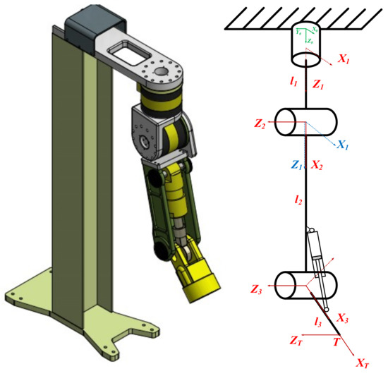
Figure 1.
The structure of the 3-DOF manipulator.
Firstly, the manipulator dynamics in the joint coordinate are expressed by:
where are position, angular velocity and angular acceleration vectors of each joint, respectively, is the symmetric and positive definite matrix of inertia, denotes the Coriolis and Centrifugal term matrix, is the gravity term, τ is torque acting on joints, is a skew-symmetric matrix [29], that is given as , and d(t) stands for the disturbance induced in the hydraulic actuator and external factor while operating.
In fact, the robot dynamic parameters are not well known. Its dynamic is affected by the mass distribution, oscillation in the process of operation. Let’s define , , where represents for estimated parameters which are clearly presented in Appendix A and acts as uncertainties of the model. Suppose that all are bounded, i.e., , then the dynamic equation of the manipulator in (1) can be rewritten as:
where denotes the uncertainties of the system.
2.2. Electro-Hydraulic Dynamics
Let represents the actuator space that is related to the robot joint-space as [Chapters 6–29]
where denotes the forward kinematics of the actuator and represents the differentiable actuator Jacobian matrix as shown in Appendix B.
The torque vector is calculated as follows [30]:
where are an area matrix of piston head part and an area matrix of rod part. are the pressure vector of two chambers of each actuator.
The hydraulic actuator pressure dynamics can be presented as follows [31]:
where is the effective bulk modulus, are volume matrix of two chambers, , is initial volumes of two chambers, are the lumped disturbances of two chambers (internal/external leakage, modelling error), is a control voltage vector, , and are flow gain coefficients matrices in orifice equations of the actuators.
where Ps and Pr are the supply pressure and the tank pressure, respectively.
2.3. State Space Form
Define the state variable vector: , . Then, the state space system is derived as follows:
where , , and .
The Equation (8) can be rewritten as follows
where , and .
Remark 1.
In practice,andare both seldom zero when the system is operating smoothly, since P1 and P2 are rarely close to Ps and Pr. In the seldom case thatandequal to zero (e.g., due to the noise in P1 and P2) it is set to a small positive number to avoid the problem of dividing zero.
3. Control Design
3.1. Sliding Mode Control with a Backstepping Technique
In this research, a robust control via the backstepping approach [19] and sliding mode control [32] is designed to control the position of the manipulator. The proposed control is divided into two control loops to control the manipulator dynamic and regulate the hydraulic dynamic. One control is a conventional sliding model [33] which handles the manipulator dynamic to generate the desired torque for the hydraulic control. In the hydraulic dynamic, an ISMC is employed to control torques under the presence of the uncertainties and the nonlinear terms.
Step 1: The sliding mode control for the manipulator dynamics.
Definite state variable errors , , and . The sliding variable vector is chosen as follows:
where is a positive-definite matrix.
The reference state of the manipulator is defined as
The derivative of the sliding variable with respect to time is expressed as follows:
Replacing (10)–(12) into the 2nd equation of (9) yields:
The desired torques are chosen as follows:
where is the positive definite matrix, is the positive definite matrix, it is chosen how to , and is a width vector, and is defined in Appendix C.
Definite the torque error vector
with .
To prove to the stability and robustness of the manipulator, the Lyapunov candidate function is chosen as follows:
The derivative of the Lyapunov functions is presented as follows:
Putting the Equations (14)–(16) into Equation (17) can yield to:
The sliding variable, , will converge to zero when the derivative of the Lyapunov function will be a negative semi-definite function. To ensure this condition, a robust control for the hydraulic dynamic is developed to guarantee that the torque error, s2, will be bounded by .
Step 2: Design the control, to assure the torque error is as small as possible. The integral sliding mode control is chosen as
where is an arbitrary positive matrix, and .
The differential of the ISMC is
The control vector is chosen
where is an arbitrary positive matrix, is a robust gain positive diagonal matrix of the sliding mode control , it is chosen how to , is a width vector, and is defined in Appendix C.
Assumption 1.
The perturbation,, varies with respect to time, and it is bounded.
Consider the Lyapunov function candidate
The derivative of the Lyapunov function (22) is
Replacing (21), and (18) into (23), the derivative of the Lyapunov function can be rewritten as follows:
where and
To guarantee the stability and robustness of the controlled system, the is a negative-definite function. The parameters , , and are chosen how the matrix is a positive definite matrix.
3.2. Proposed Control
3.2.1. Adaptive Approximation Based on RBFNN
As presented in Section 2, the uncertainties always exist in the system dynamics. They are smooth uncertanties and unsmooth uncertainties. This section presents two approximations via the Radial Basis Function Neural Network [18] to compensate the smooth uncertainties in the mechanical and hydraulic dynamics.
The RBFNN has three layers which are the input layer, hidden layer, and the output layer, which is employed to implement the approximations. The inputs and the output of the RBFNN are the tracking errors and the control input, respectively. The function of each layer is presented as follows:
The input layer rescaled the input variables, to the next layers.
The hidden layer derives the input values with the Radius Basis function, Gaussian function, as follows:
where is the input vector, , and , respectively, are the mean vector and the standard derivation of the Gaussian functions of the node ij in the hidden layer.
The output layer presents the compensation signals for the mechanical dynamic and the hydraulic dynamic as follows:
with , Each adaptive approximation includes RBFNNs and its adaptive laws and the online-tuning RBFNN is deployed to eliminate the smooth uncertainties in the mechanical dynamic and the hydraulic dynamic. These approximations reduce the chattering effects and improve the precisions. The adaptive laws are derived from the Lyapunov approach. The approximations will compensate the mechanical uncertainties and the hydraulic uncertainties such that
where are reconstructed errors; and , , and are optimal parameters of , and respectively, in the RBFNN. The approximation is expressed as the following form:
where are the estimated parameters of the RBFNN. An approximation error vector is defined as follows:
where and . The RBFs are transformed into partially linear form by the Taylor series expansion, and the can be represented as:
where ; ; is a vector of higher order terms; ; and . The equation can be rewritten as follows:
Replacing (31) into (29), it is presented that
where
3.2.2. Adaptive Sliding Mode Control with a Backstepping Technique Based on RBFNN (ABSMC)
The virtual control (14) is represented as follows:
Additionally, the control input (21) is also rewritten as follows:
Then the Lyapunov function candidate is defined as
where are positive definite matrices.
Assumption 2.
The reconstructed errors,, in the mechanical dynamics and hydraulic dynamics are bounded by.
Theorem 1.
The hydraulic manipulator is presented by (9), the indirect adaptive backstepping sliding mode control is designed by (33), (34), and the adaptive laws for the RBFNN parameters are chosen as (36)–(38) such that all the tracking error states (and) converge to zero in a finite time. The stability and robustness of the proposed control and the adaptive laws are guaranteed via the Lyapunov theory.
where,are positive definite matrices, and
The differential Lyapunov function candidate (35) is expressed as follows:
Replacing (36), (37), and (38) into (39), we have
Since and , so we have . Equation (40) can be represented as follows:
where , and .
From (41), and [34], we can conclude that the controlled system is ultimately uniformly bounded.
3.2.3. Switching Adaptive Laws
In this section, an adaptive law is developed on the robust gains to reject the unsmooth uncertainties. The adaptive laws are selected as follows:
where are threshold values of the adaptive laws, and are positive diagonal matrices, , and is estimated robust gains.
The adaptive robust gain laws (42) do not require knowledge of the upper boundary of the uncertainties. When the sliding variables stay out of a region that is smaller than , the robust gains will quickly increase to force these variables to reach to the region. Otherwise, when the variables stay in the areas, the gains will decrease rapidly. These behaviors of the robust gain can reduce the chattering effects and ensure the robustness of the system.
Proof.
The final Lyapunov function is modified as follow
The derivative of the Lyapunov function (43) is expressed as:
We consider two cases: and . When , applying (42) into (44), the derivative of a Lyapunov function is derived as follows:
It means that the Lyapunov function (43) is decreasing and bounded because .
When all sliding variables approach the small vicinity of the sliding manifold, , the derivative of a Lyapunov function is represented as:
The sliding variable will move away from the region when the derivative Lyapunov function (14) becomes positive. Then, it will become negative again when the sliding variables leave the regions and the variables are driven back toward the regions. So, we can conclude that the controlled system is uniformly asymptotically stable [34].
4. Numeral Simulation and Experimental Studies
4.1. Numerical Simulations
We conduced some simulations in MATLAB2018a with sampling time of 10−4 s and solver of ODE3. The manipulator dynamics is shown in Appendix A and Appendix B. The simulation structure is shown in Figure 2.
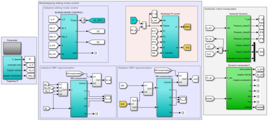
Figure 2.
Simulation structure.
The parameters of the hydraulic manipulator are shown in Table 1.

Table 1.
Parameters of the hydraulic manipulator.
To verify the effectiveness of the proposed control, some simulations are implemented under the presence of the unknown variant payload, the unknown frictions and the unknown leakages in mechanical dynamics and hydraulic dynamics. They present not only the unmatched and matched uncertainties, but also the smooth and unsmooth uncertainties. Additionally, a backstepping sliding mode control (BSMC) and PI control are also carried out and their results are compared to the proposed control (ABSMC).
The unknown frictions are expressed as:
where is a vicious positive matrix with , and is a coulomb positive matrix with .
The leakages in hydraulic dynamics are derived by
where is leakage coefficients with .
The payload is alternated as shown in Figure 3.
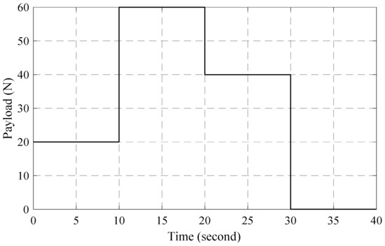
Figure 3.
Payload performance.
The reference trajectories of the hydraulic manipulator are selected as .
Each approximation in the position control has three inputs, 10 nodes in the hidden layer, and one output, and each approximation in the torque control has two inputs, 10 nodes in the hidden layer, and one output.
The parameters of the controllers are chosen by trial error method and shown in Table 2.
Table 2.
Control Parameters.
Remark 2.
In order to show the ability of the proposed control, the parameters of control are designed with payload 20 N and keep with other payloads.
Remark 3.
The proposed control is developed from the BSMC, so some parameters of SMCs in the proposed control are inherited from the BSMC.
Figure 4 and Figure 5 plots the position responses and the position errors of the joints with three controllers, PID, BSMC, and ABSMC. The results showed that the nonlinearities, uncertainties and variant payloads impacted the accuracy of the controlled system with PID control. The nonlinearities which are caused by variant payloads are dealt by the BSMC. However, the remained errors are still significant. The proposed control with adaptive laws compensated the uncertainties and improved the accuracy of the controlled system, essentially.
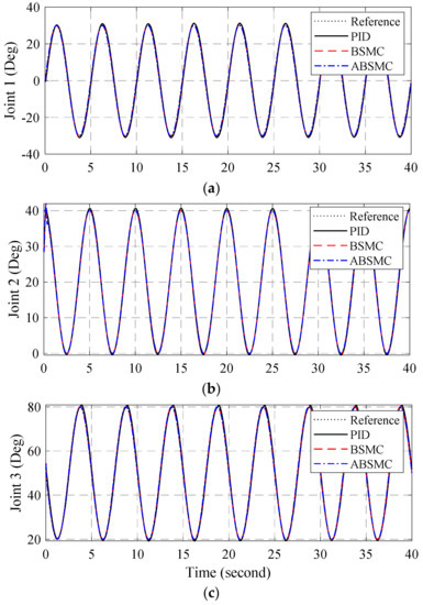
Figure 4.
Joint responses of PID, BSMC, and ABSMC in (a) joint 1, (b) joint 2, (c) joint 3.
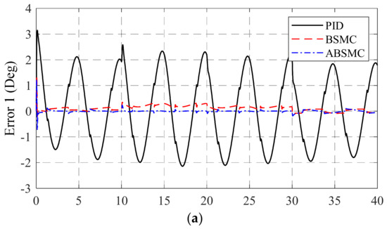
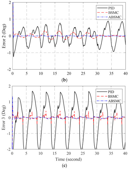
Figure 5.
Joint errors of PID, BSMC, and ABSMC in (a) joint 1, (b) joint 2, (c) joint 3.
Figure 6 and Figure 7 respectively show the torque performances and torque errors at each joint of the two controllers which are the BSMC and the proposed control. The virtual torques were calculated by (14) and (33) with the BSMC and the proposed control, respectively. The estimated torques were computed based on pressures from two chambers. The results proved that the proposed control with the adaptive mechanisms regulated the torque responses better than the BSMC. Figure 8 shows the control signals of the BSMC and the proposed controller.
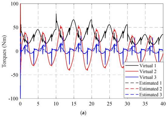
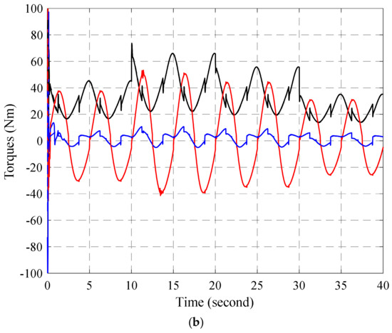
Figure 6.
Torque responses with (a) BSMC, and (b) ABSMC.
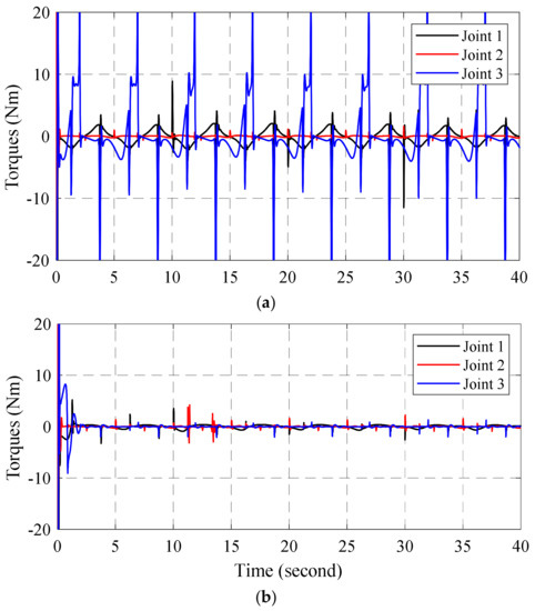
Figure 7.
Torque errors with (a) BSMC, and (b) ABSMC.
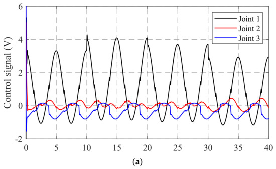
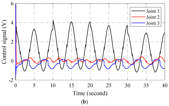
Figure 8.
Control signals of (a) BSMC, and (b) ABSMC.
Remark 4.
The simulation results proved that the proposed control compensated all uncertainties more effectiveness than the PID control and BSMC. The RBFNNs exhibited the approximately ability with the smooth uncertainties and the adaptive switching gains also demonstrate their ability for compensating the unsmooth uncertainties. However, the learning rates of adaptive laws have not mentioned in this paper. They will be intensively study in future work.
4.2. Experimental Results
Furthermore, the proposed controller and backstepping controller are practically conducted on the hydraulic manipulator with load and without load of 20 N. The test bench includes a hydraulic power, a computer and a 3-DOF manipulator as shown in Figure 9. The hydraulic flow rates which are supplied to the actuator from the hydraulic power unit are driven by the servo valves. The computer is equipped PCI cards such as PCIE 6363, and Quad04 to provide the control signal to the servo valves and read the pressure sensors and encoder sensors at each joint. The control algorithms are practically carried out in MATLAB Simulink with the Real-time Windows target toolbox at sampling time of 10 ms.
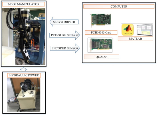
Figure 9.
Structure of the test bench.
The control parameters are set to be backstepping sliding mode control: , , , , , ; proposed control: , , , , , , , , , , , , , , , , , , .
Remark 5.
The initial weighting vectors of the RBFNNs are selected to be zero. Additionally, because the proposed control is developed based on the backstepping sliding mode control, some parameters of the proposed control are inherited from the backstepping sliding mode control.
Remark 6.
The parameters of the controllers are adjusted when the manipulator operates without load. The parameters are kept in other case.
Figure 10, Figure 11 and Figure 12 shows the joint responses, errors responses and control signals of the BSMC and proposed control when the hydraulic manipulator works without payload. In Figure 10, sinusoidal signals, (Deg.), are set up as trajectories in the joints of the hydraulic manipulator and each subfigure presents for each joint response in the manipulator. The results show that the output responses of the BSMC and the proposed control track the reference signals. In Figure 11, the error performances of joints are provided in subfigures. The results demonstrate that the proposed control approximate the uncertainties to enhance accuracy of the control performance. The Figure 12 presents the control signals of the controllers.
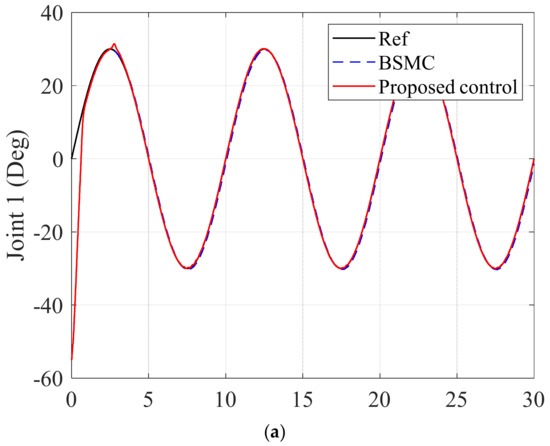
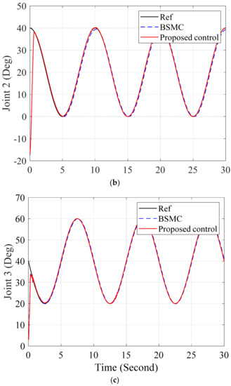
Figure 10.
Joint responses of BSMC and proposed control in (a) joint 1, (b) joint 2, (c) joint 3 without load.
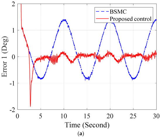
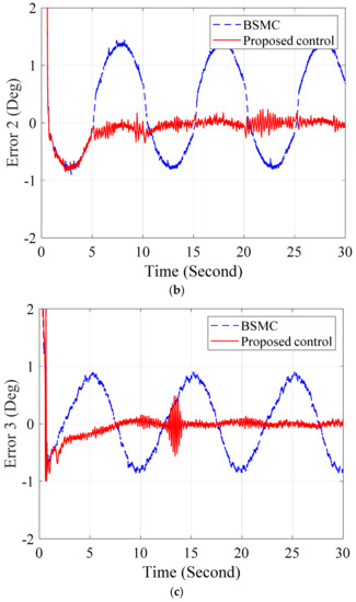
Figure 11.
Error performance of BSMC and proposed control in (a) joint 1, (b) joint2, and (c) joint 3 without load.
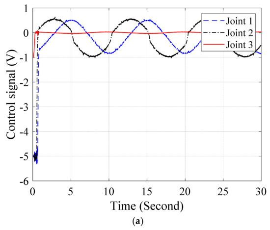
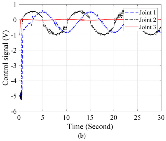
Figure 12.
Control efforts of (a) BSMC and (b) Proposed control without load.
Next experiments, the controllers are conducted on the hydraulic manipulator when the manipulator carry a payload of 20 N. The references are still sinusoidal signals as mentioned in previous case. Figure 13 and Figure 14 present the error performances and control signals of the BSMC and the proposed control. The results in Figure 13 again prove that the adaptive approximators in the proposed control compensate not only the uncertainties such as unknown friction, modeling error and leakage but also the variant payload.
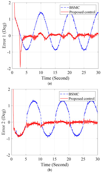
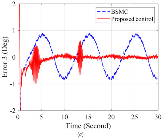
Figure 13.
Error responses of BSMC and proposed control in (a) joint 1, (b) joint 2, and (c) joint 3 with load.
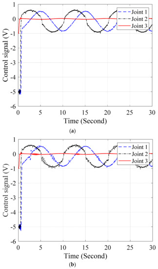
Figure 14.
Control efforts of (a) BSMC and (b) proposed control with load.
5. Conclusions
In this paper, an adaptive backstepping sliding mode control was proposed regarding tracking the position of the hydraulic manipulator including actuator dynamics under the presence of the unknown functions, the unknown variant payload, and leakages in mechanical and hydraulic dynamics. The uncertainties which present for the matched and unmatched uncertainties in the hydraulic manipulator are smooth and unsmooth functions. So, the proposition was developed based on backstepping sliding mode control, switching adaptive laws, and adaptive approximations. The adaptive approximators were developed based on RBFNN to deal with the smooth uncertainties. Specially, because the Taylor series expansion was used to analyze the RBFNN, so both the weighting vectors and parameters of the RBFs were tuning online to achieve the ideal parameters. The adaptive switching gains were provided to estimate the boundary of the unsmooth uncertainties without the predefined knowledge. The Lyapunov approach and backstepping technique were utilized together to prove the stability and robustness of the controlled system with the presence of all uncertainties. Finally, some simulations and experiments were implemented, and the results were compared to other controllers to demonstrate the effectiveness of the proposed control.
Author Contributions
K.K.A. was the supervisor providing funding and administrating the project, and he reviewed and edited the manuscript. D.-T.T. did the investigation, methodology, analysis and the validation, wrote the software, and wrote the original draft. H.-V.-A.T. checked the introduction and made the MATLAB software.
Funding
This work was supported by Basic Science Research Program through the National Research Foundation of Korea (NRF) funded by the Korean government (MEST) (NRF-2017R1A2B3004625).
Conflicts of Interest
The author declares no conflict of interest.
Appendix A
Appendix B
The relationship among the rotational motion of the joint in joint space and of its actuator space with the motion of the end-effector in Cartesian space is examined. According to Figure A1, the rotational motion is driven by the movement of the cylinder can be expressed by:
where d0 is an initial length in case of maximum retracting, d3 is the length variable when the cylinder moves, d1 and d2 are fixed length of the hinge joints. Then taking derivative of the Equation (A2), we can obtain the correlational velocity between the joint motion and the cylinder motion:
with is the Jacobian vector of the 3rd joint.
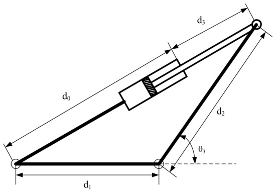
Figure A1.
The mechanical structure between the cylinder and the joint 3rd.
Then the torque acting on the 3rd joint can be deduced by:
The relationship between the actuator space and the joint space is shown as the below equations:
with are angle of the actuators in the ith (i = 1,2) joint.
The Jacobian matrix between the joint space and actuator space is depicted as follows:
Appendix C
The tan hyperbole functions are defined as follows:
where are width values.
References
- Kamezaki, M.; Iwata, H.; Shigeki, S. A practical approach to detecting external force applied to hydraulic cylinder for construction manipulator. In Proceedings of the SICE Annual Conference 2010, Taipei, Taiwan, 18–21 August 2010; pp. 1255–1256. [Google Scholar]
- Chen, Q.; Lin, T.; Ren, H. A Novel Control Strategy for an Interior Permanent Magnet Synchronous Machine of a Hybrid Hydraulic Excavator. IEEE Access 2018, 6, 3685–3693. [Google Scholar] [CrossRef]
- Altare, G.; Vacca, A.; Richter, C. A novel pump design for an efficient and compact Electro-Hydraulic Actuator. In Proceedings of the 2014 IEEE Aerospace Conference, Big Sky, MT, USA, 1–8 March 2014; pp. 1–12. [Google Scholar]
- Dong, W.; Han, S.; Jiao, Z.; Wu, S.; Zhao, Y. Compound angle-synchronizing control strategy for dual electro-hydraulic motors in hydraulic flight motion simulator. In Proceedings of the 2014 IEEE Chinese Guidance, Navigation and Control Conference, Yantai, China, 8–10 August 2014; pp. 2219–2224. [Google Scholar]
- Raibert, M.; Blankespoor, K.; Nelson, G.; Playter, R. BigDog, the Rough-Terrain Quadruped Robot. IFAC Proc. Vol. 2008, 41, 10822–10825. [Google Scholar] [CrossRef]
- Kuindersma, S.; Deits, R.; Fallon, M.; Valenzuela, A.; Dai, H.; Permenter, F.; Koolen, T.; Marion, P.; Tedrake, R. Optimization-based locomotion planning, estimation, and control design for the atlas humanoid robot. Auton. Robot. 2016, 40, 429–455. [Google Scholar] [CrossRef]
- Dollar, A.M.; Herr, H. Lower Extremity Exoskeletons and Active Orthoses: Challenges and State-of-the-Art. IEEE Trans. Robot. 2008, 24, 144–158. [Google Scholar] [CrossRef]
- Lee, J.; Chang, P.H.; Jin, M. Adaptive Integral Sliding Mode Control With Time-Delay Estimation for Robot Manipulators. IEEE Trans. Ind. Electron. 2017, 64, 6796–6804. [Google Scholar] [CrossRef]
- Van, M.; Mavrovouniotis, M.; Ge, S.S. An Adaptive Backstepping Nonsingular Fast Terminal Sliding Mode Control for Robust Fault Tolerant Control of Robot Manipulators. IEEE Trans. Syst. Manand Cybern. Syst. 2018. [Google Scholar] [CrossRef]
- Wai, R.J.; Muthusamy, R. Fuzzy-Neural-Network Inherited Sliding-Mode Control for Robot Manipulator Including Actuator Dynamics. IEEE Trans. Neural Netw. Learn. Syst. 2013, 24, 274–287. [Google Scholar] [CrossRef] [PubMed]
- Wai, R.J.; Chen, P.C. Robust Neural-Fuzzy-Network Control for Robot Manipulator Including Actuator Dynamics. IEEE Trans. Ind. Electron. 2006, 53, 1328–1349. [Google Scholar] [CrossRef]
- Wai, R.J.; Yang, Z.W. Adaptive Fuzzy Neural Network Control Design via a T-S Fuzzy Model for a Robot Manipulator Including Actuator Dynamics. IEEE Trans. Syst. Manand Cybern. Part B Cybern. 2008, 38, 1326–1346. [Google Scholar] [CrossRef]
- Wang, L.; Chai, T.; Zhai, L. Neural-Network-Based Terminal Sliding-Mode Control of Robotic Manipulators Including Actuator Dynamics. IEEE Trans. Ind. Electron. 2009, 56, 3296–3304. [Google Scholar] [CrossRef]
- Jing, Y. Adaptive control of robotic manipulators including motor dynamics. IEEE Trans. Robot. Autom. 1995, 11, 612–617. [Google Scholar] [CrossRef]
- Huang, X.; Gao, H.; Li, J.; Mao, R.; Wen, J. Adaptive back-stepping tracking control of robot manipulators considering actuator dynamic. In Proceedings of the 2016 IEEE International Conference on Advanced Intelligent Mechatronics (AIM), Banff, AB, Canada, 12–15 July 2016; pp. 941–946. [Google Scholar]
- Dinh, T.X.; Thien, T.D.; Anh, T.H.V.; Ahn, K.K. Disturbance Observer Based Finite Time Trajectory Tracking Control for a 3 DOF Hydraulic Manipulator Including Actuator Dynamics. IEEE Access 2018, 6, 36798–36809. [Google Scholar] [CrossRef]
- Huang, A. A new adaptive controller for robot manipulators considering actuator dynamics. In Proceedings of the 2018 13th IEEE Conference on Industrial Electronics and Applications (ICIEA), Wuhan, China, 31 May–2 June 2018; pp. 476–480. [Google Scholar]
- Wai, R.J.; Muthusamy, R. Design of Fuzzy-Neural-Network-Inherited Backstepping Control for Robot Manipulator Including Actuator Dynamics. IEEE Trans. Fuzzy Syst. 2014, 22, 709–722. [Google Scholar] [CrossRef]
- Krstic, M.; Kanellakopoulos, I.; Kokotovic, P.V. Nonlinear and Adaptive Control Design; Wiley: Hoboken, NJ, USA, 1995. [Google Scholar]
- Cong, B.; Liu, X.; Chen, Z. Backstepping based adaptive sliding mode control for spacecraft attitude maneuvers. Aerosp. Sci. Technol. 2013, 30, 1–7. [Google Scholar] [CrossRef]
- Ahn, K.K.; Nam, D.N.C.; Jin, M. Adaptive Backstepping Control of an Electrohydraulic Actuator. IEEE/ASME Trans. Mechatron. 2014, 19, 987–995. [Google Scholar] [CrossRef]
- Slotine, J.-J.E.; Li, W. Applied Nonlinear Control; Prentice Hall: Englewood Cliffs, NJ, USA, 1991; Volume 199. [Google Scholar]
- Huang, Y.J.; Kuo, T.C.; Chang, S.H. Adaptive Sliding-Mode Control for NonlinearSystems With Uncertain Parameters. IEEE Trans. Syst. Manand Cybern. Part B Cybern. 2008, 38, 534–539. [Google Scholar] [CrossRef]
- Chu, Y.; Fei, J.; Hou, S. Dynamic global proportional integral derivative sliding mode control using radial basis function neural compensator for three-phase active power filter. Trans. Inst. Meas. Control 2017. [Google Scholar] [CrossRef]
- Fei, J.; Lu, C. Adaptive fractional order sliding mode controller with neural estimator. J. Frankl. Inst. 2018, 355, 2369–2391. [Google Scholar] [CrossRef]
- Liu, S.; Zhou, H.; Luo, X.; Xiao, J. Adaptive sliding fault tolerant control for nonlinear uncertain active suspension systems. J. Frankl. Inst. 2016, 353, 180–199. [Google Scholar] [CrossRef]
- Li, H.; Wang, J.; Du, H.; Karimi, H.R. Adaptive Sliding Mode Control for Takagi-Sugeno Fuzzy Systems and Its Applications. IEEE Trans. Fuzzy Syst. 2018, 26, 531–542. [Google Scholar] [CrossRef]
- Zhang, Y.; Xu, Q. Adaptive Sliding Mode Control With Parameter Estimation and Kalman Filter for Precision Motion Control of a Piezo-Driven Microgripper. IEEE Trans. Control Syst. Technol. 2017, 25, 728–735. [Google Scholar] [CrossRef]
- Murray, R.M.; Li, Z.; Sastry, S.S.; Sastry, S.S. A Mathematical Introduction to Robotic Manipulation; CRC Press: Boca Raton, FL, USA, 1994. [Google Scholar]
- Yao, A.M.B. Indirect Adaptive Robust Control of Hydraulic Manipulators With Accurate Parameter Estimates. IEEE Trans. Control Syst. Technol. 2011, 19, 567–575. [Google Scholar] [CrossRef]
- Manring, N. Hydraulic Control Systems; Wiley: Hoboken, NJ, USA, 2005. [Google Scholar]
- Liu, J.; Wang, X. Adaptive Sliding Mode Control for Mechanical Systems. In Advanced Sliding Mode Control for Mechanical Systems; Springer: Berlin/Heidelberg, Germany, 2011; pp. 117–135. [Google Scholar]
- He, J.; Luo, M.; Zhang, Q.; Zhao, J.; Xu, L. Adaptive Fuzzy Sliding Mode Controller with Nonlinear Observer for Redundant Manipulators Handling Varying External Force. J. Bionic Eng. 2016, 13, 600–611. [Google Scholar] [CrossRef]
- Khalil, H.K. Nonlinear Systems; Prentice Hall: Upper Saddle River, NJ, USA, 2002. [Google Scholar]
© 2019 by the authors. Licensee MDPI, Basel, Switzerland. This article is an open access article distributed under the terms and conditions of the Creative Commons Attribution (CC BY) license (http://creativecommons.org/licenses/by/4.0/).