1. Introduction
Active noise control (ANC) over a spatially extended region, which is termed as
‘Spatial ANC’, is a challenging field of research as the aim is to create a large quiet zone for multiple listeners in three-dimensional (3-D) spaces. In spatial ANC applications, such as noise cancellation in aircraft [
1] and automobiles [
2,
3,
4,
5], multichannel ANC systems equipped with multiple sensors and multiple secondary sources are adopted [
6]. In literature, both time-domain [
7,
8] and frequency-domain [
9,
10] algorithms have been implemented in multichannel ANC systems, which can cancel the noise at error sensor positions and their close surroundings [
10]. Recently, ANC over space has been approached via Wave field synthesis (WFS)-based wave-domain algorithms [
11,
12,
13] and (cylindrical/spherical) harmonic-based wave-domain algorithms [
14,
15,
16,
17,
18,
19], with which the noise over entire region of interest can be cancelled directly. Here onwards, we use the terminology
‘wave-domain ANC’ to refer to harmonics-based wave-domain ANC.
In wave-domain ANC, the number of secondary sources/loudspeakers is required to be no less than the number of modes in the spatial region, so that all the modes can be controlled. When the number of loudspeakers cannot control all the modes in the spatial region, using the wave-domain adaptive algorithms and conventional adaptive algorithms, the noise reduction performance in the steady state degrades significantly [
16]. In practical applications, numbers and locations of the loudspeakers have more constraints compared to simulation setups in [
16]. For instance, in a vehicle, the numbers and positions of the loudspeakers are highly constrained by the vehicle dimensions and passenger convenience. It is valuable for design engineers to estimate whether the available numbers and positions of the loudspeakers are sufficient to the noise reduction requirements, before they implement an ANC system in a real environment.
Since the noise reduction performance varies with different ANC algorithms, it is important to investigate the maximum achievable performance for the given system, which is dependent on the coherence between the reference sensors and the error sensors [
20], secondary source characteristics and locations, room environments, and the primary noise field characteristics.
In the literature, Laugesen et al. provided the theoretical prediction for multichannel ANC in a small reverberant room based on the primary signal on the error sensors [
21]. For spatial ANC performance estimation over an entire region, Chen et al. investigated ANC performance by noise pattern analysis of the primary noise field [
22,
23]. Buerger et al. investigated the coherence between two observation points in the noise field evoked by given continuous source distributions, which can be applied to predict the upper bound of ANC performance in the region of interest [
24]. However, the capability of secondary sources, in particular room environments, has not yet been explored.
In this paper, we investigate the maximum noise control performance over a spatial region by investigating capability of secondary sources, in particular room environments. We define the subspace spanned by the wave-domain secondary-path coefficients, and evaluate the ANC performance in the subspace. Using the proposed subspace method, the design engineers can predict the noise cancellation performance before an actual ANC system is implemented in a product. Simulations are conducted in a 3-D room environment under different noise source positions, when the loudspeakers have constraints on numbers and positions. The proposed subspace method is more feasible than the wave-domain least squares method.
The rest of this paper is organized as follows. In
Section 2, we formulate the ANC problem in a 3-D room. We investigate the maximum ANC performance using the wave-domain least squares method in
Section 3, and investigate the maximum ANC performance using the subspace method in
Section 4. The simulation validation is demonstrated in
Section 5. We draw some conclusions in
Section 6.
2. Problem Formulation
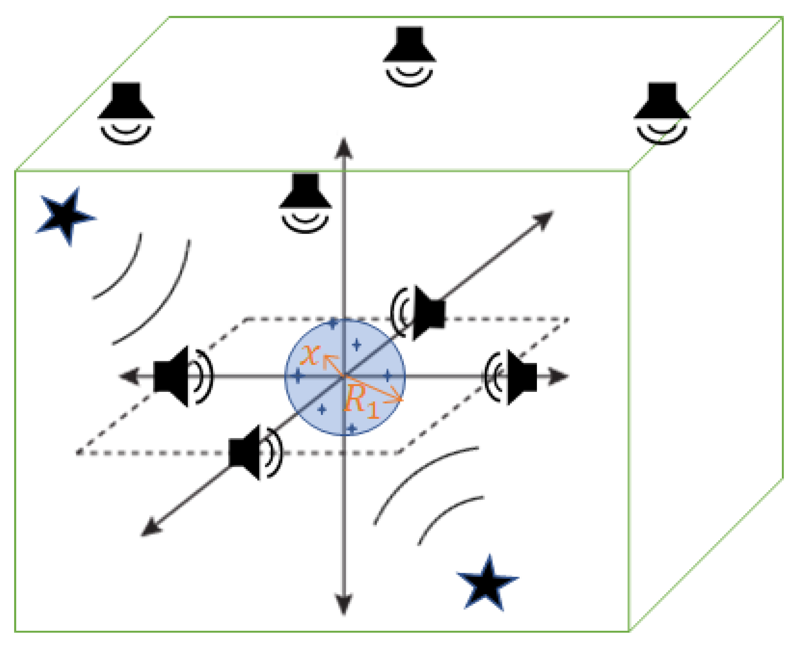
In this section, we formulate the ANC problem in the wave domain to cancel the noise over a 3-D spatial region inside rooms. As shown in
Figure 1, let the quiet zone of interest (blue area) be a spherical region (S) with a radius
. Assume that the noise sources (black stars) and the secondary sources (black loudspeakers) are located outside the region of interest. In the ANC process, we measure the noise field by placing a spherical microphone array (dark blue stars) on the boundary of the control region (i.e., the desired quiet zone).
Any arbitrary observation point within the control region is denoted as
. Here,
and
are the elevation angle and the azimuthal angle, respectively. In the ANC system, the residual signal at this point
is given by
where
is the wave number,
f is the frequency, and
c is the speed of sound propagation.
and
denote the primary noise field and the secondary noise field observed at point
, respectively.
The secondary noise field generated by a discrete loudspeaker array with
L loudspeakers (A simple model of the loudspeaker is applied here. More models characterizing the acoustic, mechanic and electric system of the loudspeakers are investigated in [
25].) can be represented by
where
is the driving signal for the
loudspeaker,
denotes the location of the
loudspeaker, and
denotes the acoustic transfer function (ATF) between the
loudspeaker and the observation point
. Please note that in the reverberant environment,
includes the room reflections.
Instead of using measurements of the microphone signals directly, the wave-domain approach employs the wave equation solutions as basis functions to express any wave field over the spatial region, and designs the secondary noise field based on the wave-domain decomposition coefficients. We then represent the primary noise field and secondary noise field in the wave domain.
The spherical harmonics-based wave equation solution decomposes any homogeneous incident wave field
observed at
into
where
is the spherical Bessel function of order
u and
denotes the spherical harmonics. Therefore, the decomposition coefficients
represent the primary noise field in the wave domain.
Within the region of interest
, a finite number of modes can be used to approximate the noise field [
26]. Thus, the primary noise field in (3) can be truncated by
where the truncation order of
[
26,
27,
28]. In the vector version,
.
Using the spherical harmonic expansion, the secondary noise field within the quiet zone can also be represented by
where the coefficients
represent the secondary noise field in the wave domain.
Similar to the primary noise field, inside the region of interest with the radius of
, the secondary noise field can be truncated by
The ATF in (2) can be parameterized in the wave domain [
29] as
where
is the ATF in wave domain for each loudspeaker.
Substituting (6) and (7) into (2), the secondary sound coefficients
can also be represented by
In matrix form, the relationship between the secondary source decomposition coefficients and the loudspeaker driving signals is given by
where
and
.
We investigate the maximum achievable ANC performance based on the primary noise field coefficients and the secondary-path information in the wave domain, and derive loudspeaker driving signals using two methods: the wave-domain least squares method and the subspace method.
3. Wave-Domain Least Squares Method
One method for deriving the loudspeaker driving signal
is to match the secondary noise field coefficients to the primary noise field coefficients, in the region of interest. Therefore,
Here, we denote the set of all linear combinations of the columns in as column space . The rank of matrix defines the dimension of the column space .
In Equation (11), (i) the number of loudspeakers, (ii) the rank of and (iii) the rank of matrix augmented by specify the number of solutions for the linear system (11).
If the number of loudspeakers is same as the number of modes in the region of interest, (11) has one unique solution, which is given by
where
denotes the inverse of a matrix.
If the number of loudspeakers is greater than the mode requirement, (11) is an under-determined system. There is either no solution or an infinite number of solutions. In practice, however, this case rarely happens, as extra loudspeakers do not result in better ANC results but increase the device cost and computational cost.
If the loudspeaker number L is less than the number of modes in the region of interest, (11) is an over-determined system. There are more equations than unknowns, resulting in either a single unique solution or no solution.
When the measurements are in a very special case, which requires
Equation (11) has an exact solution. Here, denotes the rank of , and denotes the rank of the matrix augmented by .
Equation (11) has no exact solution. The solution can be approximated using the least squares method [
30]. The least squares method tries to find the best approximation which results in minimum mean square errors [
31], by solving the following problem
The optimal solution of this minimization problem can be written as
where
denotes the pseudoinverse of a matrix.
For some circumstances,
could be totally inside the column space
. While most of time,
have components outside the space
. In general, the result of the driving signal in (16) is achieved by solving the equation as follows:
where
denotes the projected part of the primary noise field coefficients
in the column space
. The projection matrix can be also written by
In most applications, the number of loudspeakers is less than the requirement. Then the driving signals can be designed by least squares solutions in (16). Therefore, this method is here called the ‘wave-domain least squares method’ (WDLS).
4. Subspace Method
In the second method, we obtain the secondary-path coefficient , extract the subspace spanned by secondary-path coefficients which represents the secondary sources in this environment, and only cancel the primary noise field which can be projected into this subspace.
4.1. Principal Component Analysis of the Secondary Path
Let
the wave-domain secondary-path coefficients for the
loudspeaker. Matrix
in (10) for the entire loudspeaker array represents the secondary path, where
In an arbitrary loudspeaker array setup, each column of matrix is not necessarily orthogonal. We perform the principal component analysis (PCA) of the correlation matrix to obtain an orthonormal eigen-basis for the space of the secondary path in the wave domain.
We take the correlation matrix
, and then decompose this matrix into a set of orthonormal eigenvectors and their corresponding eigenvalues, as follows:
where
are the eigenvectors of the wave-domain ATF,
, and the
column corresponds to the eigenvalue
. Here onwards, the frequency dependent
k is omitted for notational simplicity. The eigenvalues in the matrix form are
Here, the vectors
are written in order of descending eigenvalues
[
32]. On this basis
, the first few largest eigenvalues correspond to the principal components of the secondary path in wave domain (
), which contain the most useful information.
Depending on the acoustic environment and the loudspeaker placement, the first
B components are used to represent the loudspeakers, then the corresponding eigenvectors are
. The subspace
O spanned by the wave-domain secondary-path coefficients
is defined as
where the dimension of
is
, and
.
By normalizing each column of matrix , the orthonormal vectors are obtained. These vectors generate a subspace, which represents the loudspeaker array and the acoustic environment. The dimensions of basis are .
For the
loudspeaker, the average ATF coefficients over certain short frames can be represented in this space as
where
are the projection coefficients. In vector form, (23) can be written by
where
and
Here, is the inner product of two vectors.
Therefore, is the secondary-path coefficients in the subspace , with the dimension of .
4.2. Projection of the Primary Noise Field into the Subspace
Below we project the wave-domain coefficients of the primary noise field into the subspace .
For a new primary noise field represented by vector
, by projecting
into the subspace
, we can obtain
where
denotes the projection of vector
into subspace
. The matrix form of the projection is represented by
where
are the primary noise field coefficients in the subspace, and
.
Therefore, the primary noise field can be separated by two parts: the projected part and the remaining part,
where
is the orthogonal complement of the subspace
. The projected part indicates the primary noise field which can be cancelled in this system setup, and the orthogonal complement indicates the primary noise field which cannot be cancelled in this system.
If , lies in the subspace, then the primary noise field can be completely cancelled by the loudspeaker array.
In more general cases, . This indicates the limitation of noise cancellation over the region of interest, under the particular loudspeaker placement and acoustic environment.
Next, we design the driving signal of loudspeaker to cancel the primary noise field projected into the subspace ().
4.3. Noise Control in the Subspace
In the subspace, matching the secondary sound field coefficients to the projected primary noise field coefficients, the optimal solution of the secondary noise field coefficients can be written by
The projection from the primary noise field into the loudspeaker subspace can be calculated by (27).
In a given loudspeaker setup, substituting (24) into (9), the representation of secondary noise field coefficients can be rewritten by
where
,
.
Substituting (27) and (30) into (29), the final equation to design the driving signal can be written as
The loudspeaker driving signals can be calculated by solving the system of linear equations described by (31). The number of principal components specifies whether the linear system (31) can be solved exactly.
Case 1:
When we reserve all the information in the PCA, (31) has only one unique solution. In that case, the driving signals can be represented by
Case 2:
When we only use the largest components to generate the subspaces, instead of solving the over-determined system in (11), Equation (31) solves an under-determined system. In that case, the driving signals
can be derived by
where
is the pseudoinverse of the secondary-path coefficients in the subspace, with the dimension of
.
In all cases, loudspeaker driving signals are designed by the secondary-path information in the subspace and the primary noise field coefficients in the subspace , as shown in (32) and (33). Therefore, the method is here called the ‘subspace method’.
5. Simulation Results
In this section, we conduct simulations to investigate the maximum achievable ANC performance in the 3-D sound field by using the WDLS and the proposed subspace method.
When the driving signal is unit amplitude, and only the loudspeaker produces sound, . Therefore, we can capture from the measurement of based on (6). For the WDLS method, the driving signals can be designed by the solutions of (11). For the subspace method, following the PCA, from (22), we can extract the subspace from the loudspeaker coefficients . Representing the in the subspace as , and projecting the primary source into the subspace as , we can derive the driving signals by solving (31).
5.1. Simulation Setup
In this simulation, we investigate the ANC performance in the reverberant environment. The reverberant environment is modelled as a cuboid room of 6 m m m. The reflection coefficients are set to [0.75, 0.8, 0.77, 0.85, 0.1, 0.1]. The reverberation is simulated by the image source method with the image order of 5. The origin of the room is on the left bottom corner. The region of interest is a spherical area with a radius of 0.5 m, and the center of the region is (3, 3, 1.5) with respect to the origin.
We assume that the noise field only contains a single-frequency component. In the following investigations, the primary noise field is a spherical wave coming from a point source located at
with respect to the center of the region, with a constant magnitude of 10. The locations of primary sources are varying in each case, as shown in
Table 1.
We assume the frequency of the noise field is 200 Hz. From (4), the region of interest in such a noise field can be represented by modes. Thus, at least microphones must be placed on the boundary to capture the information of the residual noise field for each mode. In this simulation, we place 32 microphones on the spherical boundary, following the Gauss-Legendre sampling method. White Gaussian noise is added to each microphone recording to simulate the internal thermal noise of microphones.
To control all the modes, 16 loudspeakers are required to be placed outside the control region. To emulate a practical scenario, however, in this simulation, only 12 loudspeakers are used. Among them, 8 loudspeakers are placed in the x-y plane with two different geometries, as shown in
Table 1. Another four loudspeakers are placed on another plane, which is on the plane close to the ceiling. The loudspeaker positions for each case are shown in
Table 2.
We evaluate the ANC performance in terms of residual noise field, noise reduction on the sample points inside the region , and the energy of the driving signals .
To evaluate the actual noise reduction performance within the control region, residual sound fields
at
points uniformly placed within the cross section between the region of interest and the x-y plane are examined. The noise reduction inside the region of interest over
Z points
can be written by
where
is the energy of the primary noise field at the
sample point, and
is the energy of the residual noise field at the
sample point.
To evaluate the loudspeaker energy consumption, we compare the total energy of all the loudspeakers
. The loudspeaker energy consumption can be represented by
For the subspace method, during the PCA process for the secondary path, we only reserve the principle components in . Components in which correspond to occupying less than of the largest eigenvalue are omitted in .
5.2. Cancellation Performance Using Different Methods
We first compare cancellation performance using the subspace method and the WDLS method for two different noise source positions. In this simulation, white Gaussian noise with signal to noise ratio (SNR) (Here, the SNR level is with respect to the primary noise field level on virtual microphone in the center of the region.) of 60 dB is added to each microphone recording. For simplicity of plotting, the cancellation performance over the region is confined to horizontal planes at elevation of (x-y plane) of the 3-D region.
As shown in
Figure 2, we assume noise field is generated by a point source located at (2, 315
, 45
) (case 1) or (2, 315
, 90
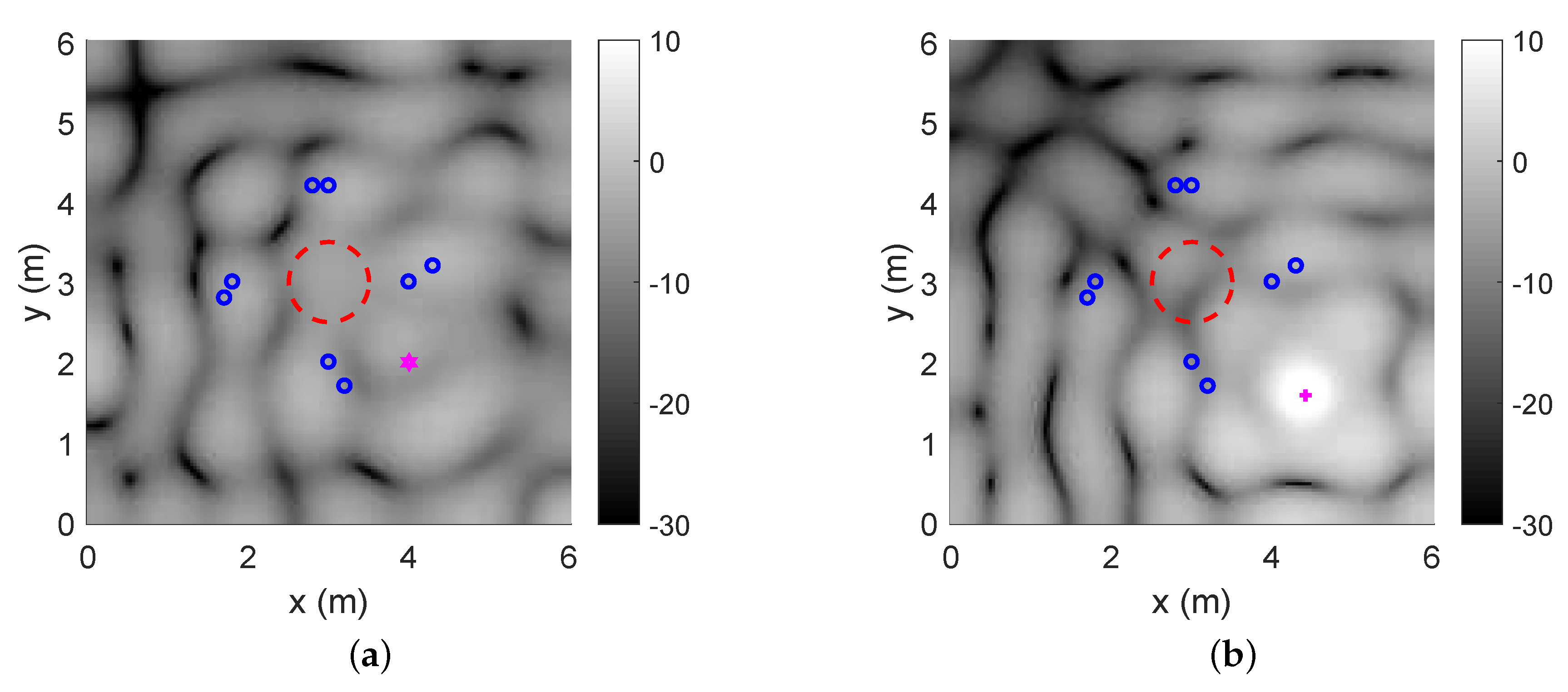
) (case 2) in the spherical coordinates. The geometry of loudspeakers in the x-y plane is not symmetrical. The energy of the primary noise field is shown in
Figure 3.
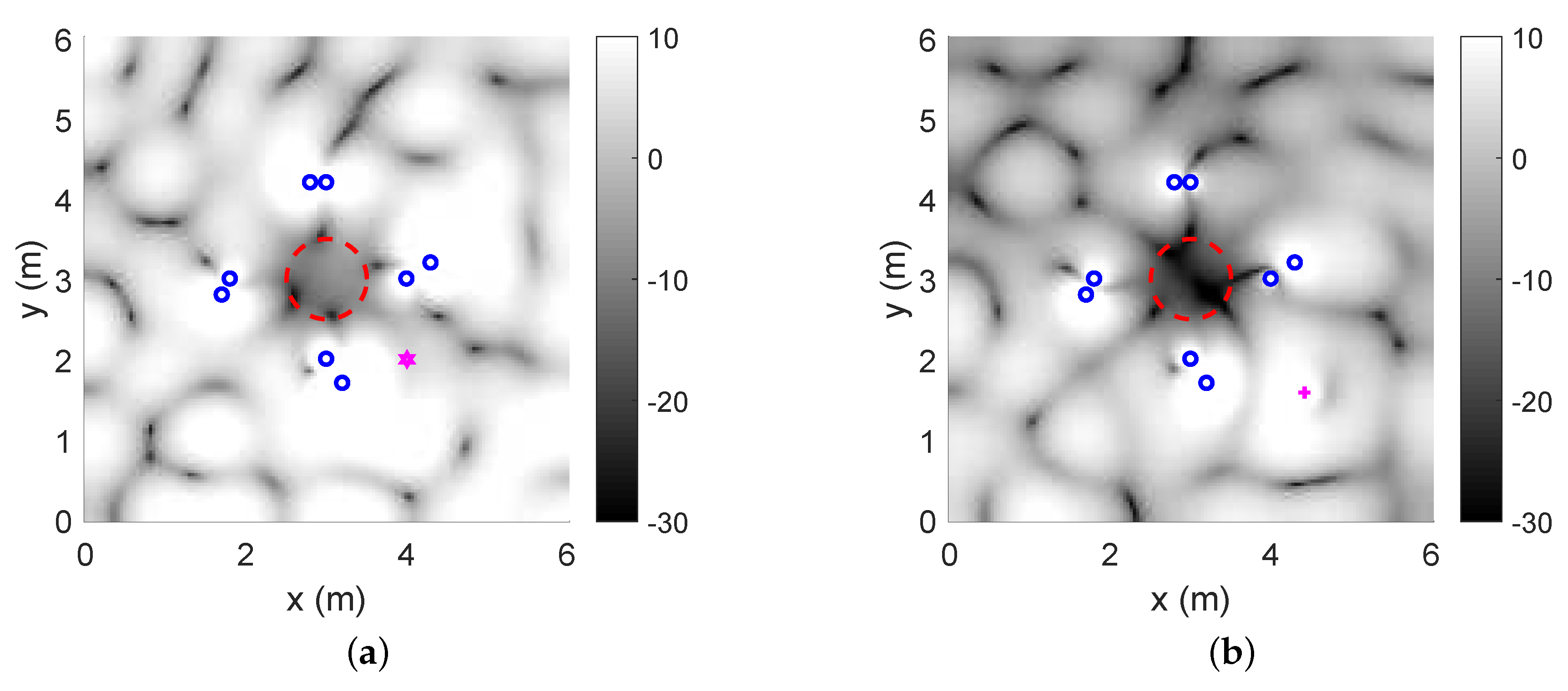
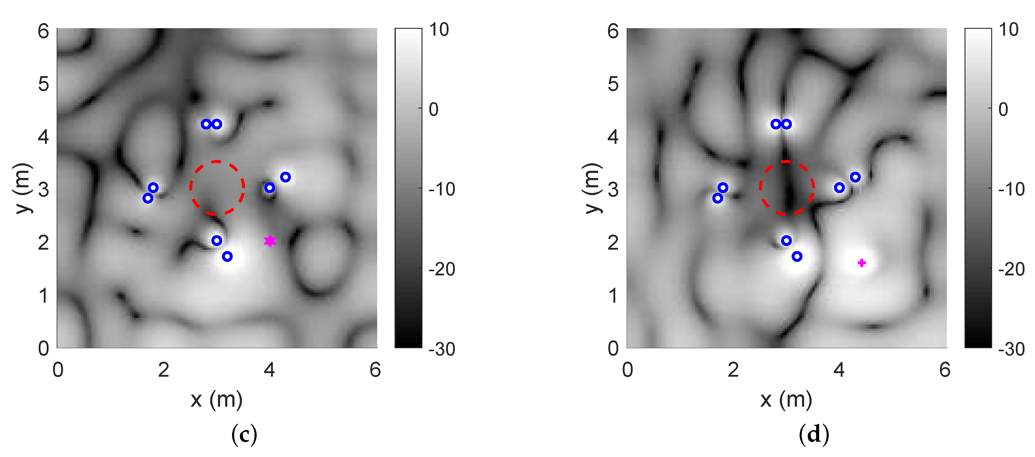
Figure 4 demonstrates the energy of the residual noise field in the x-y plane. As we expected, since the number of loudspeakers (12) cannot cover all the modes (16) in the region, in all four figures, the primary noise field in the region of interest cannot be fully cancelled. In case 2, compared with the primary noise field (
Figure 3b), both the WDLS method and the subspace method can achieve significant noise reduction in the region of interest, which are dark areas in the middle of
Figure 4b,d. In case 1, since the noise source is in a different hemisphere from the loudspeaker array, compared with
Figure 3a, cancellation performance inside the region is fairly limited for both WDLS and the subspace method, as shown in
Figure 4a,c.
Meanwhile, compared with
Figure 4a,b, in
Figure 4c,d, the subspace method results in lower energy of the residual noise field outside the region of interest. The WDLS method on the other hand produces increased sound energy outside the region, especially when the noise reduction level is fairly limited inside the region. Using the subspace method, we analyze physically achievable performance and avoid sound amplification outside the control area.
5.3. Comparison of the Effect of Different Noise Source Positions
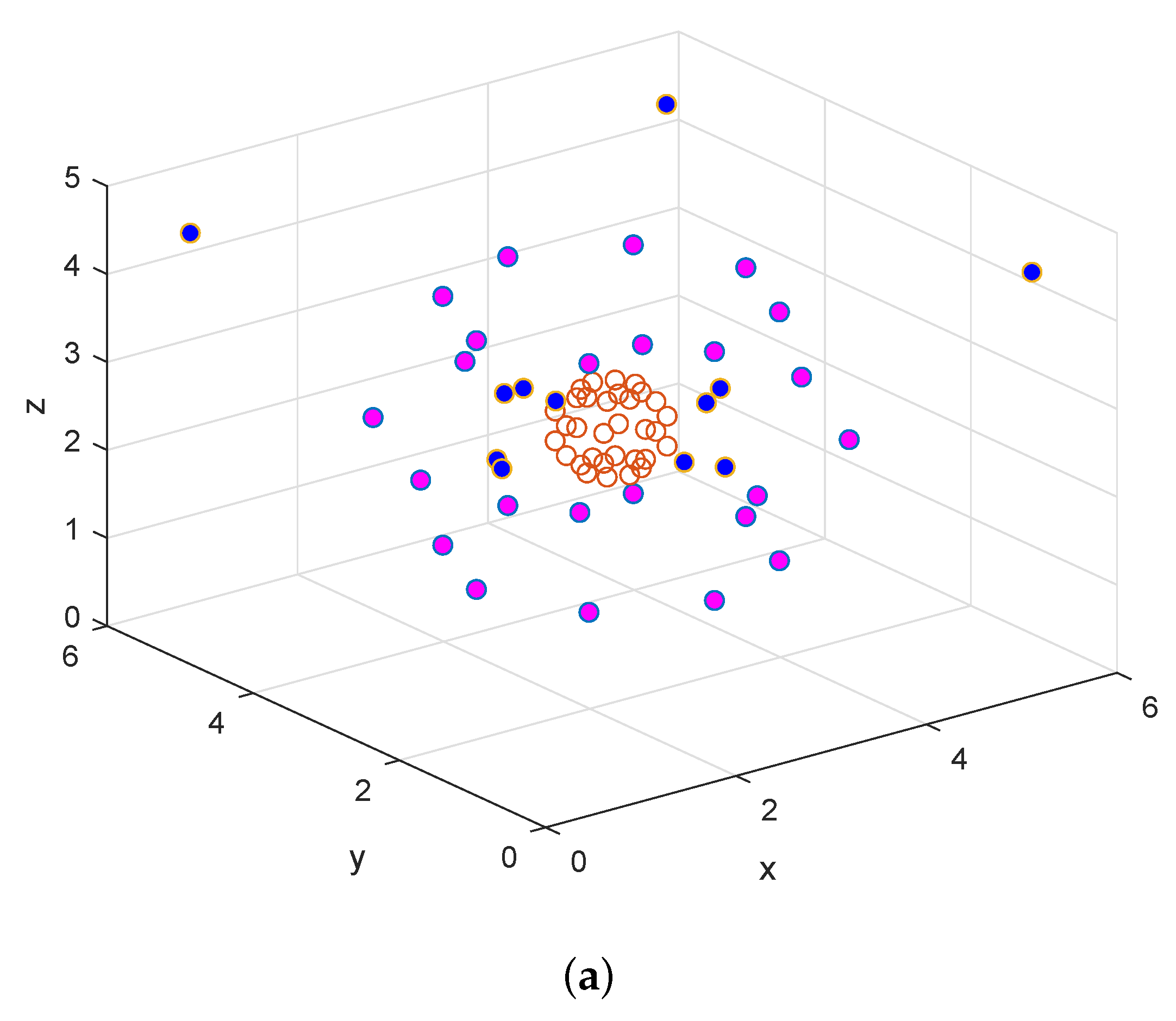
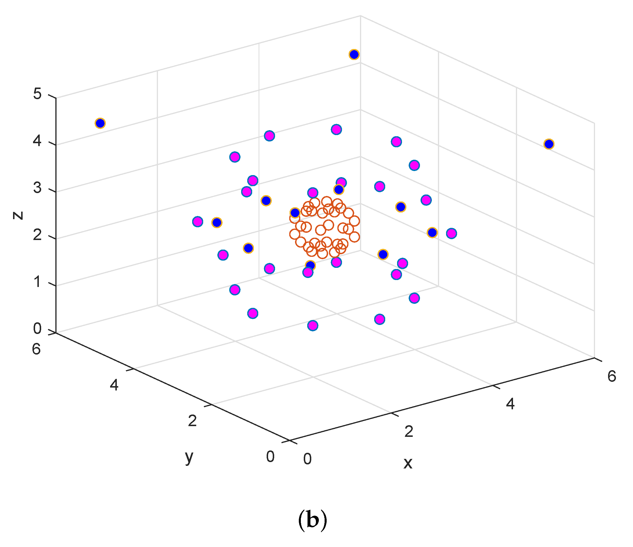
After investigating the cancellation performance in two different noise source positions, we move the noise source position to different elevations (
,
,
) and different azimuthal angles (
). As shown in
Figure 5a, 24 source position candidates are chosen on the sphere with radius of 2 m. We measure the primary noise field coefficients and secondary noise field coefficients by microphones with different SNR levels, which are 60 dB and 30 dB, respectively, for each source position candidate.
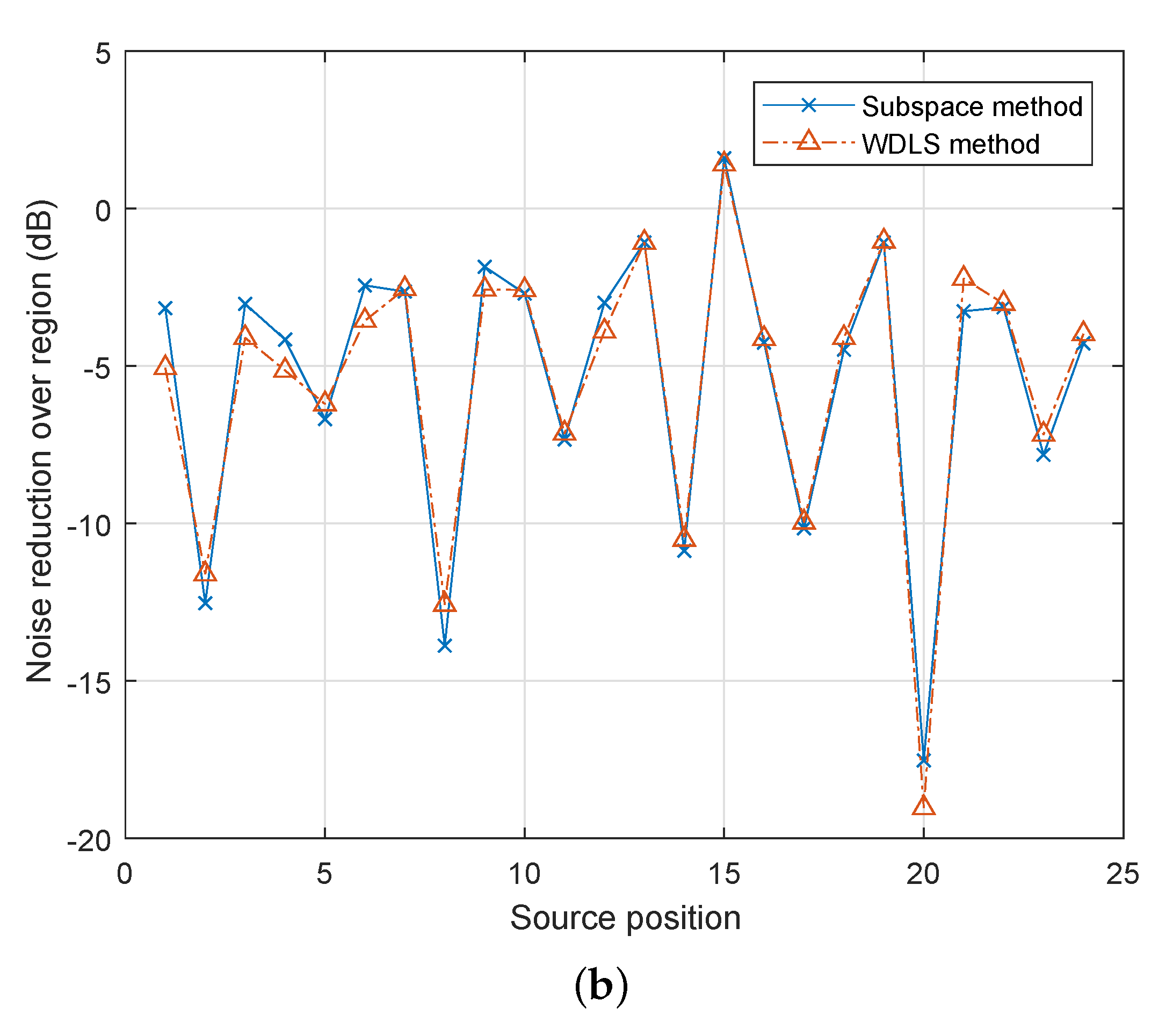
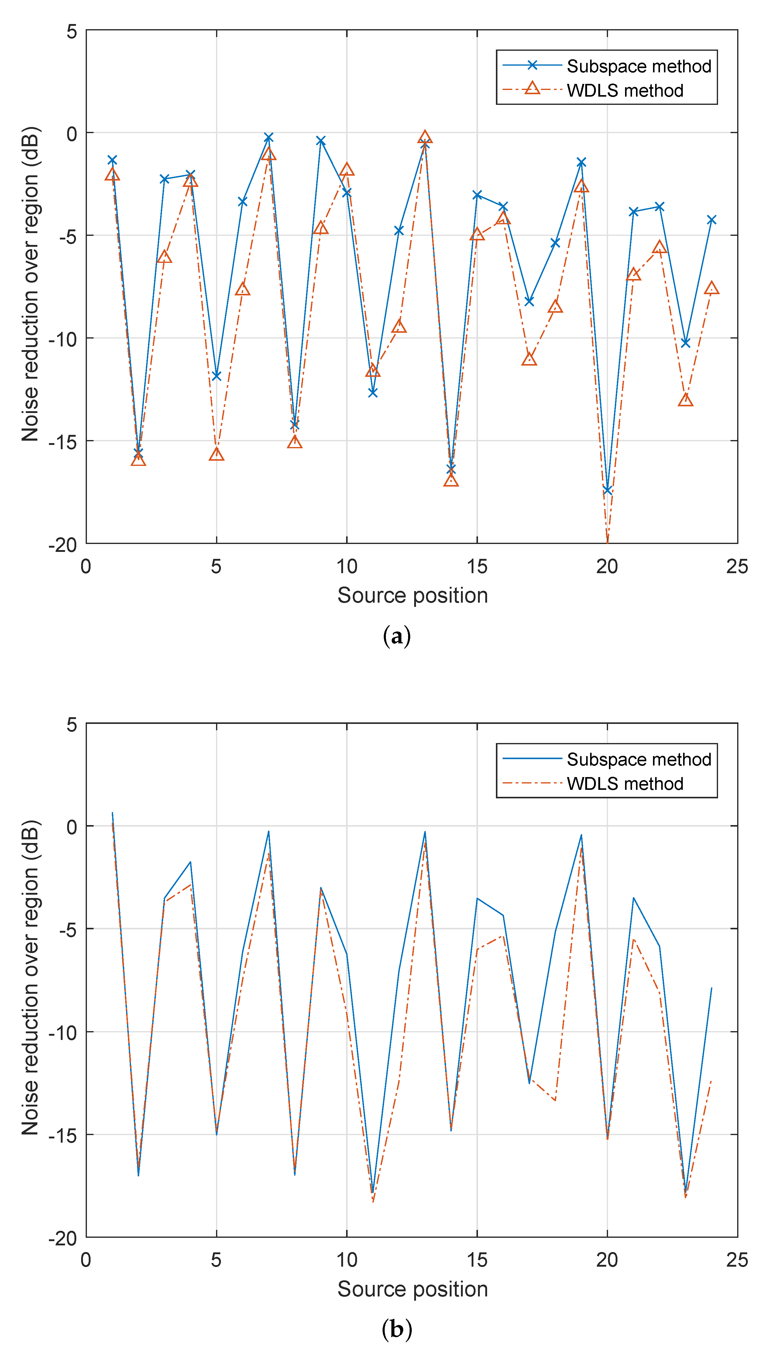
Figure 6 demonstrates the noise reduction performance for different source positions. For most of the positions, the WDLS method can achieve slightly better noise reduction than the subspace method. This is because the subspace method only uses the principal components while the WDLS method exploits all the information of the secondary path. Since 8 out of 12 loudspeakers are located in the x-y plane, the noise source positions indicated better noise reduction levels in
Figure 6a,b are position No. 2, 5, 8, 11, 14, 17, 20, 23, which are the source candidates on the x-y plane. As the accuracy of the microphone recordings is reduced, the performance prediction becomes less accurate. For example, as shown in
Figure 6b, at the noise source position 15, using both methods, the noise reduction levels are positive, which indicates the opposite result from that of
Figure 6a.
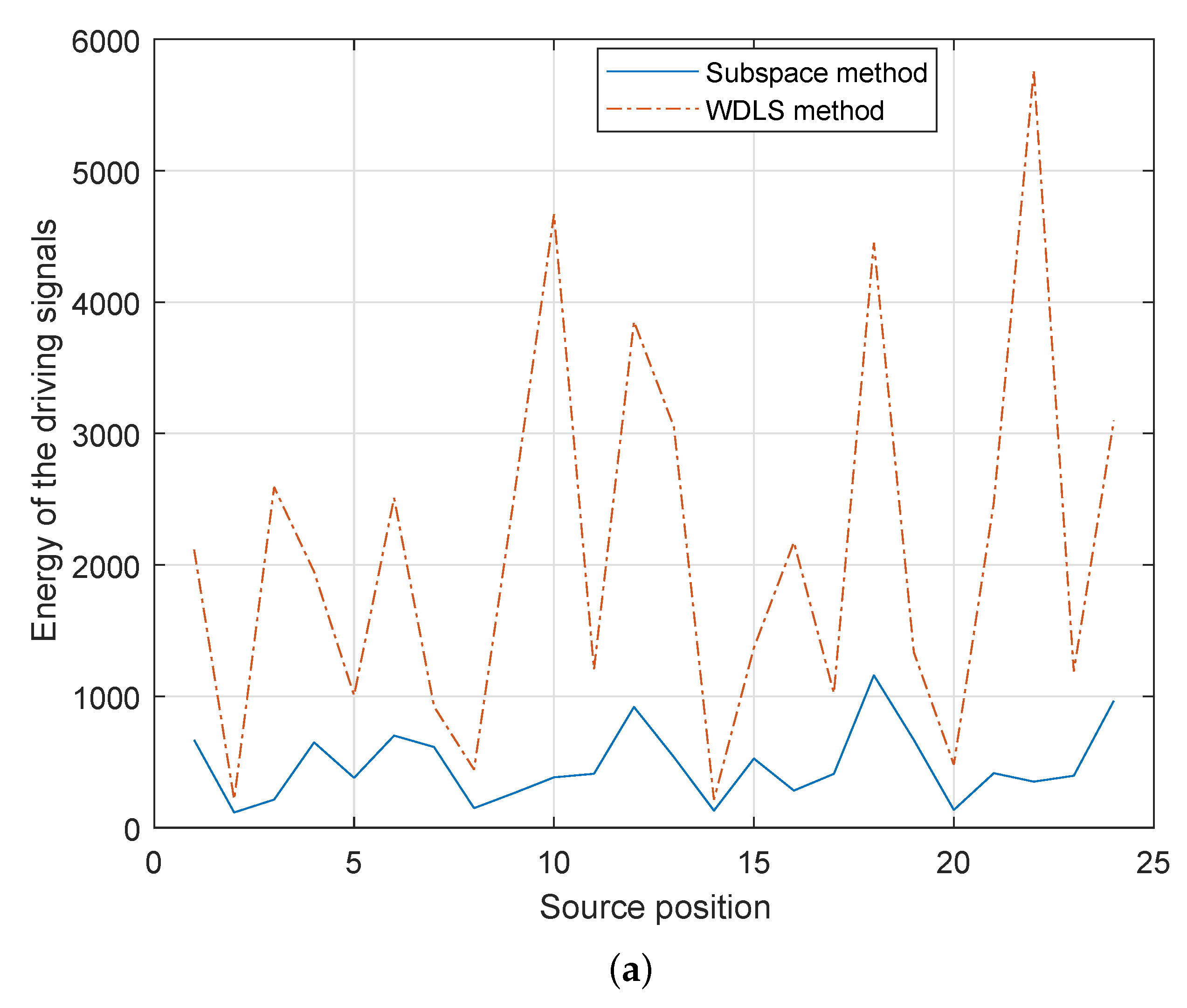
Figure 7 demonstrates the energy of the loudspeaker driving signals (
in (35)) using different methods (Here, we evaluate the summation of squared driving signals, for all the loudspeakers.). As shown in
Figure 7a,b, in both cases, compared with the WDLS method, the proposed subspace method can reduce the total energy on the loudspeakers significantly, which can avoid the overloading of the secondary sources.
5.4. Comparison of the Effect of Different Loudspeaker Placements
Since the loudspeaker placements effect the numbers of principal components in the subspace method, we investigate the noise reduction performance and energy of driving signals under different loudspeaker configurations. The ANC systems with two configurations are shown in
Figure 5. In case 4, loudspeakers in the x-y plane have symmetric geometry with respect to the control region, so that the spatial correlation between loudspeakers is greater than that in case 3 (non-symmetry).
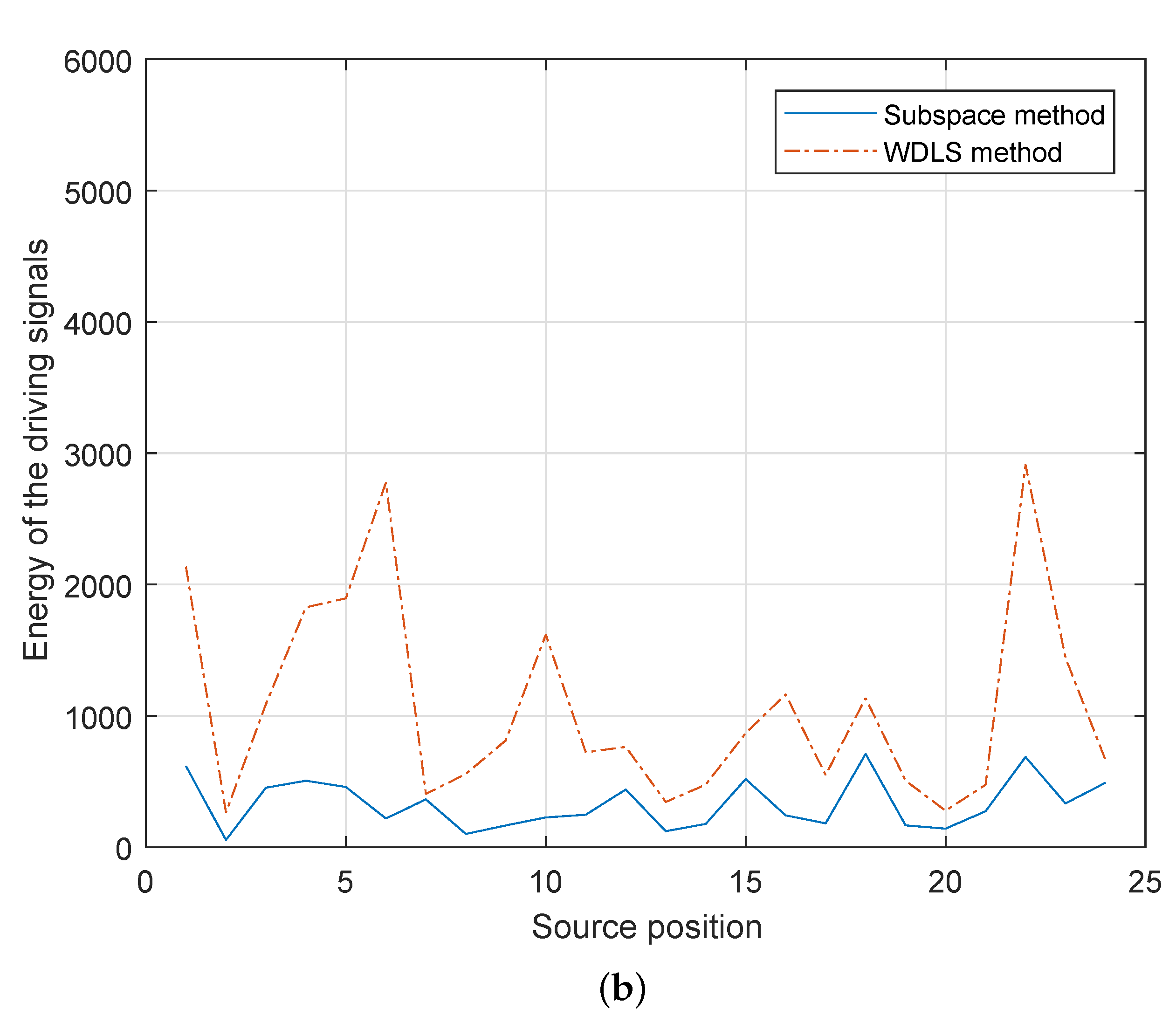
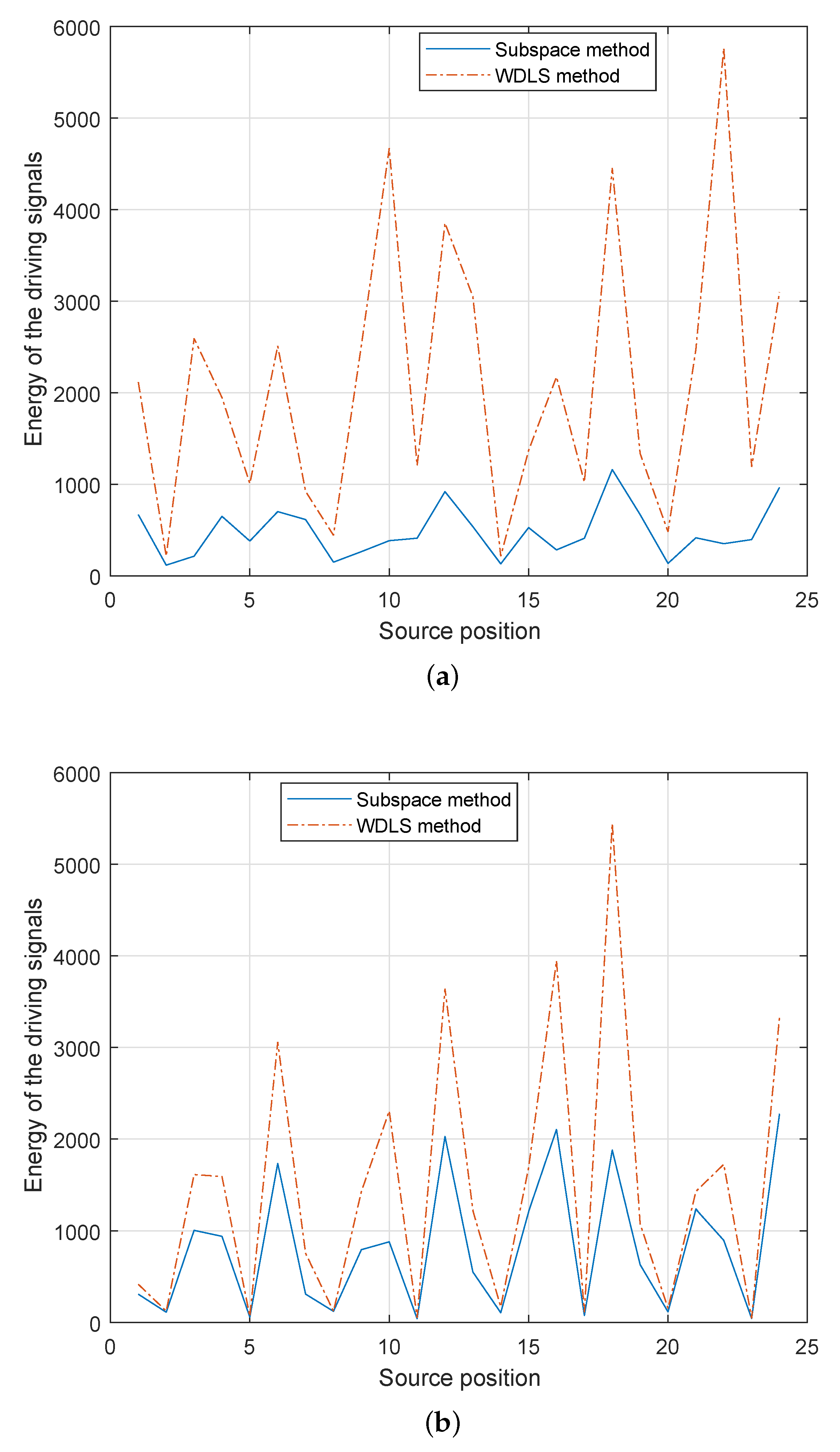
Figure 8 and
Figure 9 demonstrate the noise reduction and the energy of the loudspeaker driving signals for each noise source positions. For both loudspeaker configurations, compared with the WDLS method, the proposed subspace method achieves less noise reduction and less total energy on the loudspeakers. The significantly reduced energy of the driving signals can avoid the overloading of the secondary sources and avoid the sound amplification outside the control area. In case 3, the correlation between different loudspeakers is higher than that in case 4. In case 4, the number of principal components is larger than that in case 3. Therefore, compared with
Figure 8a and
Figure 9a, in
Figure 8b and
Figure 9b, there are less difference between the subspace method and the WDLS method.
5.5. Summary and Discussion
In summary, when the number of loudspeakers is less than the number of modes required for representing the primary noise field within the region of interest, ANC over the entire control region cannot be fully achieved. Both WDLS method and subspace method can predict the maximum achievable noise control performance over a spatial region for a given system. In most cases, the WDLS method has slightly better noise reduction performance compared to the subspace method. However, using the subspace method, both the total loudspeaker energy and the energy of the residual noise field outside the control region can be maintained at a relatively low level, which can avoid overloading of the secondary sources and sound amplification outside the control region. From the simulation results, we also notice that if the spatial correlation between different loudspeakers are small, or the accuracy of the microphone recordings are low, there are less difference between the subspace method and the WDLS method, in terms of noise reduction over the control region and energy of the loudspeakers.
6. Conclusions
In this paper, we analyzed the performance of ANC systems in 3-D reverberant environments, especially when the secondary sources have constraints on numbers and locations. We investigated the maximum achievable ANC performance based on the primary noise field and the secondary-path information in the wave domain.
We discussed a WDLS method to analyze the maximum ANC performance by matching the secondary sound field to the primary noise field in the wave domain. We proposed a subspace method to analyze the maximum ANC performance by investigating the subspace of secondary-path coefficients. We compared the proposed subspace method with the WDLS method under different loudspeaker configurations and different noise source positions, when the number of secondary sources could not control all the modes in the control region. We validated the noise reduction performance inside the control region, energy of the loudspeakers, and energy of the residual signals outside the control region.
Using the subspace method, we obtained a feasible solution with slightly lower noise reduction level inside the control region, significantly less energy on the loudspeakers, and significantly less energy on the residual noise field outside the control region. The validation with broadband noise signals and the validation with measurements in real spatial ANC applications will be conducted in the future work.
Author Contributions
Conceptualization, J.Z., T.D.A., W.Z. and P.N.S.; Funding acquisition, T.D.A., W.Z. and P.N.S.; Investigation, J.Z.; Methodology, J.Z., T.D.A., W.Z. and P.N.S.; Project administration, T.D.A.; Supervision, T.D.A., W.Z. and P.N.S.; Validation, J.Z.; Writing—original draft, J.Z.; Writing—review and editing, T.D.A., W.Z. and P.N.S.
Funding
This research was funded by ARC Discovery Project Grant number DP180102375.
Conflicts of Interest
The authors declare no conflict of interest.
Abbreviations
The following abbreviations are used in this manuscript:
| 3-D | Three-dimensional |
| ANC | Active noise control |
| ATF | Acoustic transfer function |
| PCA | Principal component analysis |
| WFS | Wave field synthesis |
| WD | Wave domain |
| WDLS | Wave-domain least squares method |
| SNR | Signal to noise ratio |
References
- Elliot, S.J.; Nelson, P.A.; Stothers, I.M.; Boucher, C.C. In-flight experiments on the active control of propeller-induced cabin noise. J. Sound Vib. 1990, 140, 219–238. [Google Scholar] [CrossRef]
- Cheer, J.; Elliott, S.J. The design and performance of feedback controllers for the attenuation of road noise in vehicles. Int. J. Acoust. Vib. 2014, 19, 155–164. [Google Scholar] [CrossRef]
- Cheer, J.; Elliott, S.J. Multichannel control systems for the attenuation of interior road noise in vehicles. Mech. Syst. Signal Process. 2015, 60, 753–769. [Google Scholar] [CrossRef]
- Samarasinghe, P.N.; Zhang, W.; Abhayapala, T.D. Recent Advances in Active Noise Control Inside Automobile Cabins: Toward quieter cars. IEEE Signal Process. Mag. 2016, 33, 61–73. [Google Scholar] [CrossRef]
- Mohammad, J.I.; Elliott, S.J.; Mackay, A. The performance of active control of random noise in cars. J. Acoust. Soc. Am. 2008, 123, 1838–1841. [Google Scholar] [CrossRef] [PubMed]
- Kajikawa, Y.; Gan, W.S.; Kuo, S.M. Recent advances on active noise control: Open issues and innovative applications. APSIPA Trans. Signal Inf. Process. 2012, 1, 21. [Google Scholar] [CrossRef]
- Barkefors, A.; Berthilsson, S.; Sternad, M. Extending the area silenced by active noise control using multiple loudspeakers. In Proceedings of the IEEE International Conference on Acoustics, Speech, and Signal Processing, Kyoto, Japan, 25–30 March 2012; pp. 325–328. [Google Scholar]
- Bouchard, M.; Quednau, S. Multichannel recursive-least-square algorithms and fast-transversal-filter algorithms for active noise control and sound reproduction systems. IEEE Trans. Speech Audio Process. 2000, 8, 606–618. [Google Scholar] [CrossRef]
- Benesty, J.; Morgan, D. Frequency-domain adaptive filtering revisited, generalization to the multi-channel case, and application to acoustic echo cancellation. In Proceedings of the IEEE International Conference on Acoustics, Speech, and Signal Processing, Istanbul, Turkey, 5–9 June 2000; Volume 2, pp. II789–II792. [Google Scholar]
- Lorente, J.; Ferrer, M.; De Diego, M.; González, A. GPU Implementation of Multichannel Adaptive Algorithms for Local Active Noise Control. IEEE/ACM Trans. Audio Speech Lang. Process. 2014, 22, 1624–1635. [Google Scholar] [CrossRef]
- Peretti, P.; Cecchi, S.; Palestini, L.; Piazza, F. A Novel Approach to Active Noise Control Based on Wave Domain Adaptive Filtering. In Proceedings of the 2007 IEEE Workshop on Applications of Signal Processing to Audio and Acoustics (WASPAA), New Paltz, NY, USA, 21–24 October 2007; pp. 307–310. [Google Scholar] [CrossRef]
- Spors, S.; Buchner, H. An approach to massive multichannel broadband feedforward active noise control using wave-domain adaptive filtering. In Proceedings of the 2007 IEEE Workshop on Applications of Signal Processing to Audio and Acoustics (WASPAA), New Paltz, NY, USA, 21–24 October 2007; pp. 171–174. [Google Scholar] [CrossRef]
- Spors, S.; Buchner, H. Efficient massive multichannel active noise control using wave-domain adaptive filtering. In Proceedings of the 3rd International Symposium on Communications, Control and Signal Processing, St Julians, Malta, 12–14 March 2008; pp. 1480–1485. [Google Scholar]
- Zhang, J.; Zhang, W.; Abhayapala, T.D. Noise Cancellation over Spatial Regions using Adaptive Wave Domain Processing. In Proceedings of the IEEE Workshop on Applications of Signal Processing to Audio and Acoustics, New Paltz, NY, USA, 18–21 October 2015; pp. 1–5. [Google Scholar]
- Zhang, J.; Abhayapala, T.D.; Samarasinghe, P.N.; Zhang, W.; Jiang, S. Sparse complex FxLMS for active noise cancellation over spatial regions. In Proceedings of the IEEE International Conference on Acoustics, Speech and Signal Processing (ICASSP), Shanghai, China, 20–25 March 2016; pp. 524–528. [Google Scholar]
- Zhang, J.; Abhayapala, T.D.; Zhang, W.; Samarasinghe, P.N.; Jiang, S. Active Noise Control Over Space: A Wave Domain Approach. IEEE/ACM Trans. Audio Speech Lang. Process. 2018, 26, 774–786. [Google Scholar] [CrossRef]
- Zhang, W.; Hofmann, C.; Buerger, M.; Abhayapala, T.D.; Kellermann, W. Spatial Noise-Field Control With Online Secondary Path Modeling: A Wave-Domain Approach. IEEE/ACM Trans. Audio Speech Lang. Process. 2018, 26, 2355–2370. [Google Scholar] [CrossRef]
- Maeno, Y.; Mitsufuji, Y.; Abhayapala, T.D. Mode Domain Spatial Active Noise Control Using Sparse Signal Representation. In Proceedings of the 2018 IEEE International Conference on Acoustics, Speech and Signal Processing (ICASSP), Calgary, AB, Canada, 15–20 April 2018; pp. 211–215. [Google Scholar] [CrossRef]
- Maeno, Y.; Mitsufuji, Y.; Samarasinghe, P.N.; Abhayapala, T.D. Mode-Domain Spatial Active Noise Control Using Multiple Circular Arrays. In Proceedings of the 2018 16th International Workshop on Acoustic Signal Enhancement (IWAENC), Tokyo, Japan, 17–20 September 2018; pp. 441–445. [Google Scholar] [CrossRef]
- Kuo, S.M.; Morgan, D. Active Noise Control Systems: Algorithms and DSP Implementations; John Wiley & Sons, Inc.: Hoboken, NJ, USA, 1995. [Google Scholar]
- Laugesen, S.; Elliott, S.J. Multichannel active control of random noise in a small reverberant room. IEEE Trans. Speech Audio Process. 1993, 1, 241–249. [Google Scholar] [CrossRef]
- Chen, H.; Samarasinghe, P.N.; Abhayapala, T.D. In-car noise field analysis and multi-zone noise cancellation quality estimation. In Proceedings of the 2015 Asia-Pacific Signal and Information Processing Association Annual Summit and Conference (APSIPA), Hong Kong, China, 16–19 December 2015; pp. 773–778. [Google Scholar] [CrossRef]
- Chen, H. Theory and Design of Spatial Active Noise Control Systems. Ph.D. Thesis, The Australian National University, Canberra, Australia, 2017. [Google Scholar]
- Buerger, M.; Abhayapala, T.D.; Hofmann, C.; Chen, H.; Kellermann, W. The spatial coherence of noise fields evoked by continuous source distributions. J. Acoust. Soc. Am. 2017, 142, 3025–3034. [Google Scholar] [CrossRef] [PubMed]
- Bianco, F.; Teti, L.; Licitra, G.; Cerchiai, M. Loudspeaker FEM modelling: Characterisation of critical aspects in acoustic impedance measure through electrical impedance. Appl. Acoust. 2017, 124, 20–29. [Google Scholar] [CrossRef]
- Kennedy, R.; Sadeghi, P.; Abhayapala, T.D.; Jones, H.M. Intrinsic Limits of Dimensionality and Richness in Random Multipath Fields. IEEE Trans. Signal Process. 2007, 55, 2542–2556. [Google Scholar] [CrossRef]
- Abhayapala, T.D.; Pollock, T.; Kennedy, R. Characterization of 3D spatial wireless channels. In Proceedings of the 2003 IEEE 58th Vehicular Technology Conference VTC 2003-Fall, Orlando, FL, USA, 6–9 October 2003; Volume 1, pp. 123–127. [Google Scholar]
- Kennedy, R.A.; Abhayapala, T.D. Spatial Concentration of Wave-Fields: Towards Spatial Information Content in Arbitrary Multipath Scattering. In Proceedings of the 4th Australian Communications Theory Workshop (AusCTW 2003), Australian National University, Canberra, Australia, 4 February 2003; pp. 38–45. [Google Scholar]
- Betlehem, T.; Abhayapala, T.D. Theory and design of sound field reproduction in reverberant rooms. J. Acoust. Soc. Am. 2005, 117, 2100–2111. [Google Scholar] [CrossRef] [PubMed]
- Golub, G.H.; Van Loan, C.F. Matrix Computations; JHU Press: Baltimore, MD, USA, 1996; pp. 236–247. [Google Scholar]
- Parodi, Y.L.; Rubak, P. Objective evaluation of the sweet spot size in spatial sound reproduction using elevated loudspeakers. J. Acoust. Soc. Am. 2010, 128, 1045–1055. [Google Scholar] [CrossRef] [PubMed]
- Wold, S.; Esbensen, K.; Geladi, P. Principal component analysis. Chemom. Intell. Lab. Syst. 1987, 2, 37–52. [Google Scholar] [CrossRef]
Figure 1.
ANC system in a 3-D room. Black stars represent primary sources, loudspeakers represent secondary sources, the blue sphere represents the control region, and dark blue stars represent error microphones over the control region.
Figure 1.
ANC system in a 3-D room. Black stars represent primary sources, loudspeakers represent secondary sources, the blue sphere represents the control region, and dark blue stars represent error microphones over the control region.
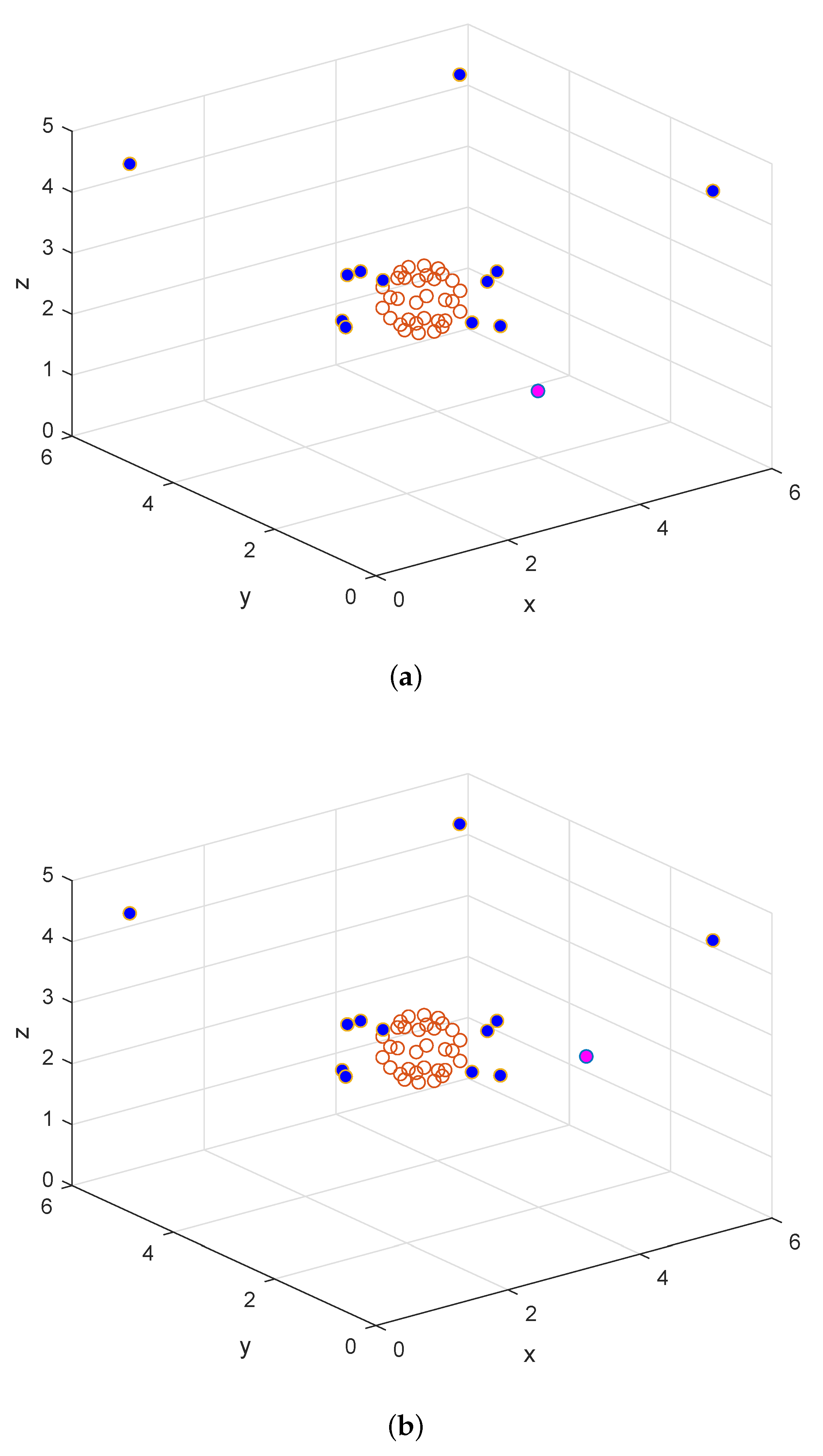
Figure 2.
ANC system setup, where the pink point is the noise source position, blue points are loudspeaker positions, and red points are microphone positions: (a) case 1; (b) case 2.
Figure 2.
ANC system setup, where the pink point is the noise source position, blue points are loudspeaker positions, and red points are microphone positions: (a) case 1; (b) case 2.
Figure 3.
Energy of the primary noise field, where pink point is the projection of the primary source on the x-y plane, blue points are the loudspeaker points located on the x-y plane, and the red dashed circle is the boundary of the region of interest: (a) case 1; (b) case 2.
Figure 3.
Energy of the primary noise field, where pink point is the projection of the primary source on the x-y plane, blue points are the loudspeaker points located on the x-y plane, and the red dashed circle is the boundary of the region of interest: (a) case 1; (b) case 2.
Figure 4.
Energy of the residual noise field, when the noise field is generated by one primary source
using different methods. Here, pink point is the projection of the primary source on the x-y plane and
blue points are the loudspeaker points located on the x-y plane: (a) the WDLS method in case 1; (b) the
WDLS method in case 2; (c) the subspace method in case 1; (d) the subspace method in case 2.
Figure 5.
Two different array setups, when the noise source moves around a sphere, where in both
setups, pink points are the primary source positions, blue points are loudspeaker positions, and red
points are microphone positions: (a) Case 3; (b) Case 4.
Figure 5.
Two different array setups, when the noise source moves around a sphere, where in both
setups, pink points are the primary source positions, blue points are loudspeaker positions, and red
points are microphone positions: (a) Case 3; (b) Case 4.
Figure 6.
Noise reduction performance in case 3, when the noise field is generated by one primary
source moving around the sphere using different methods: (a) with SNR = 60 dB white noise on the microphone recordings; (b) with SNR = 30 dB white noise on the microphone recordings.
Figure 6.
Noise reduction performance in case 3, when the noise field is generated by one primary
source moving around the sphere using different methods: (a) with SNR = 60 dB white noise on the microphone recordings; (b) with SNR = 30 dB white noise on the microphone recordings.
Figure 7.
Energy of the driving signals in case 3, when the noise field is generated by one primary
source moving around the sphere using different methods: (a) with SNR = 60 dB white noise on the microphone recordings; (b) with SNR = 30 dB white noise on the microphone recordings.
Figure 7.
Energy of the driving signals in case 3, when the noise field is generated by one primary
source moving around the sphere using different methods: (a) with SNR = 60 dB white noise on the microphone recordings; (b) with SNR = 30 dB white noise on the microphone recordings.
Figure 8.
Noise reduction over the region using different loudspeaker setups, when the noise field generated by one primary source moving around the sphere using different methods: (a) case 3; (b) case 4.
Figure 8.
Noise reduction over the region using different loudspeaker setups, when the noise field generated by one primary source moving around the sphere using different methods: (a) case 3; (b) case 4.
Figure 9.
Energy of the driving signals generated by one primary source moving around the sphere using different methods: (a) case 3; (b) case 4.
Figure 9.
Energy of the driving signals generated by one primary source moving around the sphere using different methods: (a) case 3; (b) case 4.
Table 1.
Loudspeaker array setup and noise source location in 4 cases, which are given in Figures 2 and 5, respectively.
Table 1.
Loudspeaker array setup and noise source location in 4 cases, which are given in Figures 2 and 5, respectively.
| Loudspeaker Array | Non-Symmetry | Symmetry |
|---|
| Noise Source Position | |
|---|
| case 1 | |
| case 2 | |
| 24 position candidates | case 3 | case 4 |
Table 2.
Loudspeaker positions for non-symmetric placement and symmetric placement.
Table 2.
Loudspeaker positions for non-symmetric placement and symmetric placement.
| Loudspeakers in the x-y Plane | Loudspeakers Outside the x-y Plane |
|---|
| No. | Non-Symmetry | Symmetry | No. | Non-Symmetry or Symmetry |
|---|
| 1 | (4, 3, 2.5) | (4.5, 3, 2.5) | 9 | (0.5, 0.5, 4.5) |
| 2 | (1.8, 3, 2.5) | (1.5, 3, 2.5) | 10 | (5.5, 5.5, 4.5) |
| 3 | (3, 2, 2.5) | (3, 1.5, 2.5) | 11 | (5.5, 0.5, 4.5) |
| 4 | (3, 4.2, 2.5) | (3, 4.5, 2.5) | 12 | (0.5, 5.5, 4.5) |
| 5 | (4.3, 3.2, 2.5) | (4.2, 1.8, 2.5) | | |
| 6 | (1.7, 2.8, 2.5) | (1.8, 1.8, 2.5) | | |
| 7 | (3.2, 1.7, 2.5) | (4.2, 4.2, 2.5) | | |
| 8 | (2.8, 4.2, 2.5) | (1.8, 4.2, 2.5) | | |
© 2019 by the authors. Licensee MDPI, Basel, Switzerland. This article is an open access article distributed under the terms and conditions of the Creative Commons Attribution (CC BY) license (http://creativecommons.org/licenses/by/4.0/).


