Change Detection of Water Resources via Remote Sensing: An L-V-NSCT Approach

Abstract

Aiming at the change detection of water resources via remote sensing, the non-subsampling contour transformation method combining a log-vari model and the Stractural Similarity of Variogram (VSSIM) model, namely log-vari and VSSIM based non-subsampled contourlet transform (L-V-NSCT) approach, is proposed. Firstly, a differential image construction method based on non-subsampled contourlet transform (NSCT) texture analysis is designed to extract the low-frequency and high-frequency texture features of the objects in the images. Secondly, the texture features of rivers, lakes and other objects in the images are accurately classified. Finally, the change detection results of regions of interest are extracted and evaluated. In this experiment, the L-V-NSCT approach is compared with other methods with the results showing the effectiveness of this method. The change in Dongting Lake is also analyzed, which can be used as a reference for relevant administrative departments.

1. Introduction

With improvement in the level of software and hardware for remote sensing acquisition along with the increase in the quantity of data, the need for change detection is also increasing, and the requirements for precision are getting higher and higher. Remote sensing plays an important role in water environment monitoring. In disaster prevention and mitigation, water conservation involves flood and waterlogging disasters, drought and wading geological disaster monitoring and assessment, flood forecasting and early warning. In water resource monitoring and protection, it involves satellite remote sensing precipitation forecasts, soil moisture and evapotranspiration remote sensing estimation, surface water monitoring, groundwater monitoring, water environment monitoring and surface water body monitoring. With respect to ecological protection, water conservation involves the monitoring of the environment, the investigation of soil and water conservation and irrigation area, the monitoring and control of river course and estuary change.

In lake water area change detection, remote sensing technology is used to monitor lake area change. On the one hand, the law along with the trend of annual and interannual changes in the lake area should be analyzed from a natural point of view to better protect lakes through watershed management. On the other hand, we must supervise the illegal occupation of water in real time to provide clues for law enforcement. In the Hubei Province, China, from January to July 2015, nearly 48 suspected illegal spots were found in lake monitoring by remote sensing. Law enforcement departments checked 15 suspected illegal spots in the field and confirmed seven real illegal events. This work will be further extended to the monitoring of reservoirs and rivers. In addition, surface water monitoring is also an important part of drought monitoring.

In the remote sensing of water resources, Xu et al. [1] used the NDWI model to extract the water bodies of the Tangjiashan barrier lake from the multisource satellite images to detect the changes in the barrier lake, pre- and post-earthquake. Qiao et al. [2] compared paleo lakes with modern lakes, showing that lakes on the Tibetan Plateau have shrunk significantly since the great lake period, which provides fundamental information to support research on both global paleo-climatology and paleo-hydrology change. Zhao et al. [3], by combining ecological quantity analysis with GIS technology based on land use data and remote sensing imagery, analyzed the changes in land use and land cover as well as the driving force in the mainstream of the Tarim River from 1973 to 2005. Markogianni et al. [4] used Landsat and Systeme Probatoire d’Observation de la Terre (SPOT) images to estimate the Normalized Difference Vegetation Index (NDVI) and land-use changes at the Plastira artificial lake catchment for the period 1984–2009. Adesina et al. [5] focused on change detection on the Jebba Lake Basin between 1978 (five years before the dam was established) and 1995 (twelve years after the dam impoundment). Refice et al. [6] applied high-resolution, X-band, and stripmap Cosmo-SkyMed data to the monitoring of flood events in the Basilicata region (Southern Italy). By using the mapping results with post-earthquake high-resolution images from Google Earth, Zhao et al. [7] showed that the pixel-based landslide mapping method was able to identify landslides with relatively high accuracy. Sun et al. [8] used Cosmo-Skymed ScanSAR mode (HH) data for one-year monitoring of seasonal changes in the water surface areas of Poyang Lake from January 2014 to December 2014. Li et al. [9] proposed a change detection method based on Gabor wavelet features for very high resolution (VHR) remote sensing images. The fuzzy c-means cluster algorithm was employed to obtain the final change map. Setiawan et al. [10] implemented the canny edge detection method, combining with Otsu thresholding to detect the edges, achieved good edge detection results.

Gao et al. [11] presented a change detection method for multitemporal synthetic aperture radar images based on PCANet and exploited representative neighborhood features from each pixel using PCA filters as convolutional filters. Zhao et al. [12] proposed a difference image analysis approach based on deep neural networks for use on image change detection problems. Gong et al. [13] put forward a novel approach for change detection in SAR images. This approach classified changed and unchanged regions by fuzzy c-means (FCM) clustering with a Markov random field (MRF) energy function.

At present, commonly used change detection methods are not accurate enough to detect the edge contours of rivers, lakes, urban roads, and forest vegetation in severely damaged areas and there are too many small areas of debris in the disaster areas, which are judged as image changes. At the same time, the impact of this noise will lead to high error rates and false alarm rates.

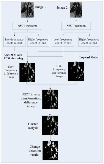
To dynamically monitor the changes of inland surface resources such as Ocean Lake wetlands and lake swamps, this paper proposes an L-V-NSCT approach based on the NSCT and the logarithmic variation function. Firstly, NSCT transform was used to decompose the detected image and the VSSIM algorithm was used to extract the texture information difference at different scales after multi-scale decomposition. Secondly, the texture difference images of rivers, lakes and other objects were fused by utilizing the NSCT inverse transform. Finally, the spectral information, texture information, and space of the objects were fully considered. The fuzzy c-means clustering model (CFCM) was designed to classify the difference features of the above images.

The experiments in subsequent chapters can prove the effectiveness of the method. At the same time, the greatest innovation of this method was that it has good practicability and has been applied in the protection of Dongting Lake. On the basis of the GF-2 image, the method regularly provided the relevant departments with test results and reference.

2. Directional Logarithmic Variogram and the VSSIM Model

At present, variogram analysis [14,15] is typically used to study the texture structure and spatial correlation of an entire image. This paper mainly uses a variation function to consider the structural characteristics of surface features in different period’s images and highlights the edge contour structure of target features such as rivers and lakes in images, as well as the variation characteristics of the main edges in the detection area. Based on the classic mathematical model of the variogram, a logarithmic variogram model with horizontal (0°), vertical (90°), and diagonal (45°, 135°) directions was proposed. The model can quickly locate and analyze the main edge contour information of image objects.

Set $f(x,y)$ as the size of the collected image M × N; the sliding window with the designed width $L=2d+1$ was designed to analyze and process different types of ground object data in the image source. The center pixel of the ground object in the window can be set as $(i_0,j_0)$, the coordinates of the ground object pixels in other positions can be set as $(i,j)$, and the edge analysis model (log-vari) of the directional logarithmic variation function can be set as follows:

$${r_h}^0(i_0,j_0)=\frac{1}{2N_0(h)}{\displaystyle \sum _{i-i_0-d}^{i_0+d}{\displaystyle \sum _{j-j_0-d}^{j_0+d-h}|\ln [f(i,j)]-\ln [f(i,j+h)]|}}$$

(1)

$${r_h}^{45}(i_0,j_0)=\frac{1}{2N_{45}(h)}{\displaystyle \sum _{i-i_0-d}^{i_0+d-h}{\displaystyle \sum _{j-j_0-d}^{j_0+d-h}|\ln [f(i,j+h)]-\ln [f(i+h,j)]|}}$$

(2)

$${r_h}^{90}(i_0,j_0)=\frac{1}{2N_{90}(h)}{\displaystyle \sum _{i-i_0-d}^{i_0+d-h}{\displaystyle \sum _{j-j_0-d}^{j_0+d}|\ln [f(i,j)]-\ln [f(i+h,j)]|}}$$

(3)

$${r_h}^{135}(i_0,j_0)=\frac{1}{2N_{135}(h)}{\displaystyle \sum _{i-i_0-d}^{i_0+d-h}{\displaystyle \sum _{j-j_0-d}^{j_0+d-h}|\ln [f(i,j)]-\ln [f(i+h,j+h)]|}}$$

(4)

where $f(i,j+h)$ and $f(i,j)$ are two coordinate values with distance h in the area. The values of the directional value $\theta$ are {0°, 45°, 90°, 135°}. $N_{\theta }(h)$ is the number of all two-coordinate points in the region with a distance of h, and the final output mathematical matrix sequence $r^{\theta }(x,y)$ is the texture coefficient matrix in the direction of $\theta$.

In the process of feature similarity analysis, the structure similarity model (SSIM) can be constructed from the brightness, contrast, and structure factor of the image [16]. The expression is as follows:

$$SSIM(x,y)={[l(x,y)]}^{\alpha }·{[c(x,y)]}^{\beta }·{[s(x,y)]}^{\gamma }$$

(5)

where $l(x,y)$ is the luminance coefficient matrix, $c(x,y)$ is the contrast parameter, and $s(x,y)$ is the structural parameter. The parameters $\alpha ,\beta ,\gamma$ are all less than 1.

To improve the detection accuracy of texture details of different types of objects in seismic images and the clearer edge structure of lakes and rivers, we used the edge texture coefficient matrix obtained in the upper section to improve and optimize the SSIM model and propose the structure of directional logarithmic variogram model similarity (VSSIM).

We selected two images of size M × N, which are represented by X and Y. First, the average value of the edge texture $r^{\theta }(x,y)$ of the two images was calculated by using the log-vari model in the direction of $\theta$. The extracted edge texture feature coefficients are $r_X(x,y)$ and $r_Y(x,y)$. At the same time, the structural similarity algorithm $v(x,y)$ of the logarithmic variation function was constructed to judge the change degree of edge features in the texture feature matrix.

$$v(x,y)=\frac{k{\displaystyle \sum _{j=1}^M{\displaystyle \sum _{i=1}^N[r_X(i,j)\times r_Y(i,j)}]+c_1}}{{\displaystyle \sum _{j=1}^M{\displaystyle \sum _{i=1}^N{[r_X(i,j)]}^2+{\displaystyle \sum _{j=1}^M{\displaystyle \sum _{i=1}^N{[r_Y(i,j)]}^2+c_2}}}}}$$

(6)

Through these experiments, we found that the optimal values of the parameters in the above expressions were generally $k$ = 2, $c_1$ = $c_2$ = 0.001.

In the SSIM expression, the structure factor $s(x,y)$ can be replaced by the edge structure factor $v(x,y)$. The constructed an edge structure similarity model (VSSIM) based on the logarithmic variation function is expressed as follows:

$$VSSIM(x,y)={[l(x,y)]}^{\alpha }·{[c(x,y)]}^{\beta }·{[v(x,y)]}^{\gamma }$$

(7)

3. Differential Image Construction

By using edge texture enhancement, the goal of change detection with the logarithmic variation function was to construct more accurate image difference features in the process of NSCT multiscale transformation. The main steps were as follows:

(1) NSCT multiscale transform of the original image; the multiscale NSCT transform was used to obtain low-frequency texture coefficients and high-frequency texture coefficients in different scales. The expressions are as follows:

$$NSCT(I_1)=\{L_1,{H_1}^{1,1},{H_1}^{1,2},\dots ,{H_1}^{1,k}\}$$

(8)

$$NSCT(I_2)=\{L_2,{H_2}^{1,1},{H_2}^{1,2},\dots ,{H_2}^{1,k}\}$$

(9)

where $L_1(x,y)$ and $L_2(x,y)$ are the low-frequency coefficient matrices of the two-period images, and ${H_1}^{l,k}(x,y)$ and ${H_2}^{l,k}(x,y)$ are the high-frequency coefficient matrices in the $k$th direction of the first level in the multiscale decomposition process.

(2) Construction of the low-frequency texture difference coefficient $L(x,y)$ in the NSCT domain; after $I_1$ and $I_2$ decomposition, the low-frequency features $L_1(x,y)$ and $L_2(x,y)$ were extracted. VSSIM was used to measure the difference in the low-frequency texture features, and the coefficient matrix $vssim(x,y)$ of low-frequency texture similarity was extracted. Then, the coefficient matrix was used to weigh the low-frequency texture difference to obtain the feature difference. Finally, threshold and FCM clustering were used to extract the low-frequency texture feature difference image $L(x,y)$.

$$L(x,y)=\mathrm{FCM}[\left|L_1(x,y)-L_2(x,y)\right|\times vssim(x,y)]$$

(10)

(3) Construction of the high-frequency texture difference coefficient $H^{l,k}(x,y)$ in the NSCT domain; the log-variogram was used to analyze high-frequency texture features and to extract the high-frequency edge texture coefficient matrix ${r_1}^{l,k}(x,y)$ and ${r_2}^{l,k}(x,y)$. These texture coefficients were used to calculate the similarity coefficient matrix $s^{l,k}(x,y)$ of high-frequency texture and to judge the degree of difference of high-frequency texture features in these scale-space images. Finally, FCM clustering was used to extract the high-frequency edge difference texture features.

$$s^{l,k}(x,y)={\displaystyle \sum _{i=1}^M{\displaystyle \sum _{j=1}^N\{1-\frac{\left|{r_1}^{l,k}(i,j)-{r_2}^{l,k}(i,j)\right|}{\max [{r_1}^{l,k}(i,j),{r_2}^{l,k}(i,j)]}\}}}$$

(11)

The difference coefficient expression of high-frequency edge texture features in NSCT domain is as follows:

$$H^{l,k}(x,y)=\mathrm{FCM}[\left|{H_1}^{l,k}(x,y)-{H_2}^{l,k}(x,y)\right|\times s^{l,k}(x,y)]$$

(12)

(4) Construction of image texture difference features based on the NSCT transform; the low-frequency texture difference coefficients $L(x,y)$ and high-frequency texture difference coefficients $H^{l,k}(x,y)$ on different scales were extracted. The NSCT inverse transform was used to construct texture difference images $D(x,y)$ of multi-temporal remote sensing images.

$$D(x,y)=NSCTRE\{L(x,y),H^{l,k}(x,y)\}$$

(13)

4. Difference Image Clustering

To improve the classification accuracy of remote sensing images, an improved fuzzy C-means clustering method (CFCM) was used based on the degree of correlation. Firstly, the correlation between image data were accurately described by the similarity between their key feature vectors. The improved weighted coefficient similarity measure takes the similarity degree between the central vertex ${\mathrm{O}}_{\mathrm{i}}$ and the neighboring vertex ${\mathrm{O}}_{\mathrm{j}}$ as the $\mathrm{weight}({\mathrm{e}}_{ij})$ of any edge ${\mathrm{e}}_{ij}$ in a 3 × 3 sliding window.

$$\mathrm{weight}({\mathrm{e}}_{ij})={\displaystyle \sum _{k=1}^3\frac{1}{1+m_i\times \left|d_{ik}-d_{jk}\right|}}$$

(14)

where m_i is a coefficient, and the values of k and i belong to {1,2,3}. Secondly, the weight of an edge ${\mathrm{e}}_{ij}$ of the center vertex ${\mathrm{O}}_{\mathrm{i}}$ of the texture information in the window was calculated.

$$k_{ij}=\frac{\mathrm{weight}({\mathrm{e}}_{ij})}{{\displaystyle \sum _{{\mathrm{e}}_{ij}\in E}\mathrm{weight}({\mathrm{e}}_{ij})}}$$

(15)

Next, the correlation degree of data objects based on pixel $D(x,y)$ in difference images was calculated.

$$\mathrm{Cor}({\mathrm{D}}_i)={\displaystyle \sum _{{\mathrm{e}}_{ij}\in E}\{k_{ij}\times \mathrm{weight}({\mathrm{e}}_{ij})}\}$$

(16)

FCM clustering was then used to accurately classify the correlation degree of all data objects in the extracted differential images.

$$D(p,q)=\{\begin{array}{l}{w}_c,\mathrm{Cor}({\mathrm{D}}_{\mathrm{i}})>T_1\\ w_n,T_2\le \mathrm{Cor}({\mathrm{D}}_{\mathrm{i}})\le T_1\\ w_u,\mathrm{Cor}({\mathrm{D}}_{\mathrm{i}})<T_2\end{array}$$

(17)

where $w_c,w_n,w_u$ denote change class, fuzzy class and invariant class, respectively. $T_1,T_2$ are thresholds. Lastly, a region growing method was used to optimize the classification results of CFCM based on the classified difference features and the appropriate threshold processing was used to extract more accurate change detection results.

5. Experimental Results and Analysis

To verify the effectiveness of the L-V-NSCT method proposed in this paper, we used real datasets to conduct experiments and analyze the results. Before the change detection, we first carried out the image gray normalization, texture enhancement, and other preprocessing. The flow chart of L-V-NSCT change detection is shown in Figure 1.

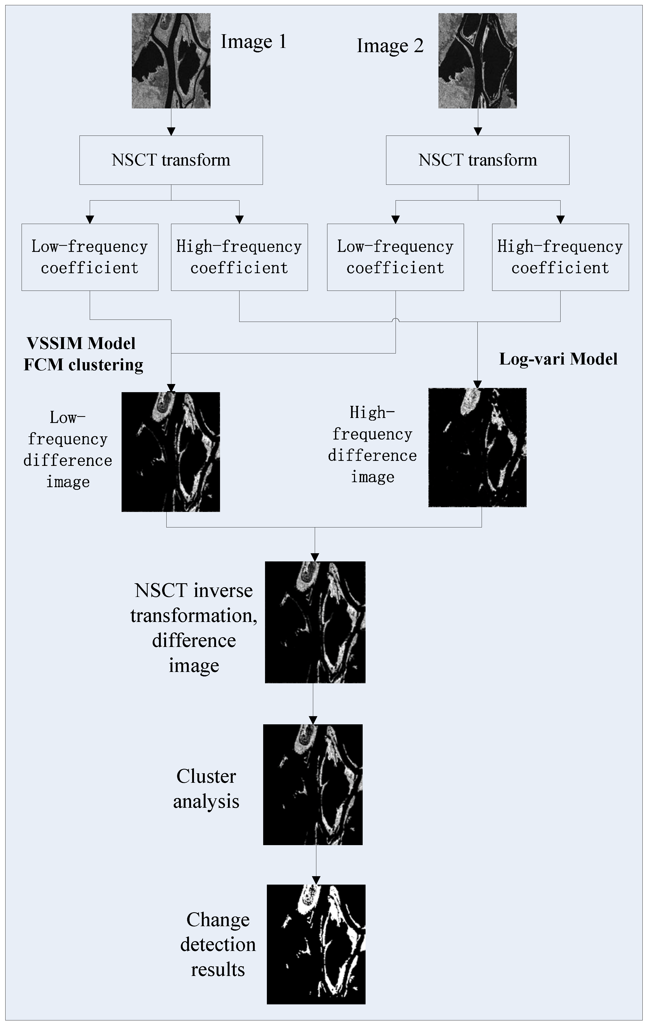
We first detected the changes of lakes and water bodies in Sardinia area [17], as shown in Figure 2. The size of the image was 412 × 300. The comparison algorithms were NSCTKFCM [18] and NSCTFCM [19], both of which were improvements of the NSCT algorithm. Figure 2a is the image of the Sardinia region in April 1999, Figure 2b is the image of the Sardinia region in May 1999, Figure 2c is the result of the NSCTKFCM method, Figure 2d is the result of the NSCTFCM method, Figure 2e is the result of L-V-NSCT and Figure 2f is the reference image of the result, where the number of changed pixels was 7626.

From the results, we can see that three detection algorithms achieved good results for the change detection of rivers and lakes in the image. However, the other two algorithms were greatly affected by noise, the edges of the river change areas were blurred, and the fragments change areas (areas of no concern) caused by false alarm were relatively increased. Nonetheless, the L-V-NSCT approach can effectively preserve the details of the change area and show that the edge of the main change area is clear. The above experiments showed that L-V-NSCT approach has some advantages in detecting changes in remote sensing images.

In the experiment, we found that the indexes of the L-V-NSCT approach were different when different types of images were analyzed. For low-brightness images, the bit error rate of change detection increased, and the accuracy decreased.

Radarsat images of Ottawa, Canada, from May 1997 and August 1997 were the original images of the dataset in the second experiments [11,12,13], as shown in Figure 3. The image size is 290 × 350, and the number of changed pixels is 16049.

Figure 4 shows the low-frequency difference image, the high-frequency difference image, and the final detection result. Figure 4a,b are the low-frequency difference image based on the logarithmic variation function and the low-frequency difference coefficient image after further clustering, respectively. Figure 4c is the high-frequency difference coefficient image after similarity analysis. Figure 4d is the NSCT inverse transform fusion image. Figure 4e is the clustering result image, and Figure 4f is the last change detection binary image.

As seen from the images, L-V-NSCT can detect the changes in the registered images very well, and the details are relatively complete.

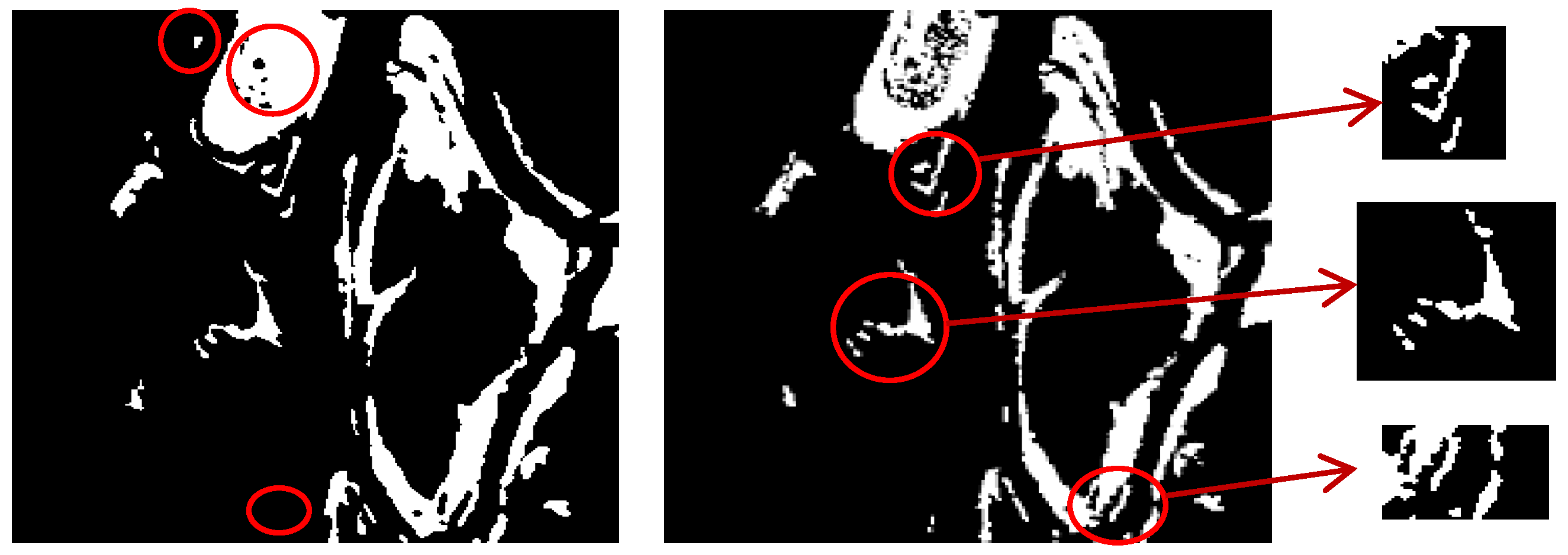
Figure 5 further reflects the detail effect of L-V-NSCT change detection. The left image is the manual labeled change detection reference image, and the right image is the detection result of this method. The labeling parts in the right figures show that the proposed method can obtain results consistent with the manual judgment in most local areas. The left parts with circles are marked with false alarm or missing alarm areas, which need further analysis and judgment. Therefore, we will further compare the indicators with other methods.

We used statistical accuracy (PCC) and Kappa index (KC) as experimental indicators to evaluate the performance of the algorithm [12]. If FP is the number of the pixels belonging to the unchanged class but falsely classified as the changed class, and FN is the number of the pixels belonging to the changed class but falsely classified as the unchanged class. TP and TN represent the number of changed pixels and unchanged pixels that are correctly detected, respectively. Then the correct classification accuracy (PCC) is:

$$PCC=\frac{TP+TN}{N}$$

(18)

where $N$ is the total number of pixels in the image. And the Kappa index KC is calculated as:

$$KC=\frac{PCC-PRE}{1-PRE}$$

(19)

where $PRE=\frac{(TP+FP)\times (TP+FN)+(FN+TN)\times (FP+TN)}{N^2}$.

In the experimental comparison, besides NSCTKFCM and NSCTFCM, the L-V-NSCT method was also compared with other methods in recent years, namely PCANet [11], DNN [12], and MRFFCM [13]. The experimental results are shown in

Table 1. Change detection results under evaluation by different algorithms.

Method	PCC (%)	FN	FP	KC
NSCTKFCM	95.24	2085	2749	0.8241
NSCTFCM	97.51	236	2286	0.9113
PCANet	98.22	944	863	0.9300
DNN	98.09	1059	883	0.9278
MRFFCM	97.69	712	1636	0.9151
L-V-NSCT	98.36	948	681	0.9379

.

From the data analysis in Table 1, we can see that both the PCC and KC of L-V-NSCT were higher than the other five approaches. Although the FN of L-V-NSCT was higher than NSCTFCM, MRFFCM and PCANet, the FP was comparatively lower. So, the final PCC and KC of L-V-NSCT were also better than that of the 3 algorithms.

We also conducted experiments with 20 of our remote sensing image databases, with the average accuracy and Kappa index obtained are shown in

Table 2. Average results of change detection by different methods.

Method	PCC (%)	KC
NSCTKFCM	82.63	0.5527
NSCTFCM	84.51	0.7816
PCANet	90.78	0.8569
DNN	91.57	0.8932
MRFFCM	88.34	0.8544
L-V-NSCT	92.96	0.8845

. As can be seen from the table, among all the six methods, NSCTKFCM performed the worst and the experimental results were unstable. The experimental results of PCANet, DNN and L-V-NSCT were better. DNN, in particular, performed very well due to the use of deep neural networks. The performance of L-V-NSCT was relatively stable. Although KC of L-V-NSCT was slightly lower than that of DNN, the PCC was still higher than that of DNN.

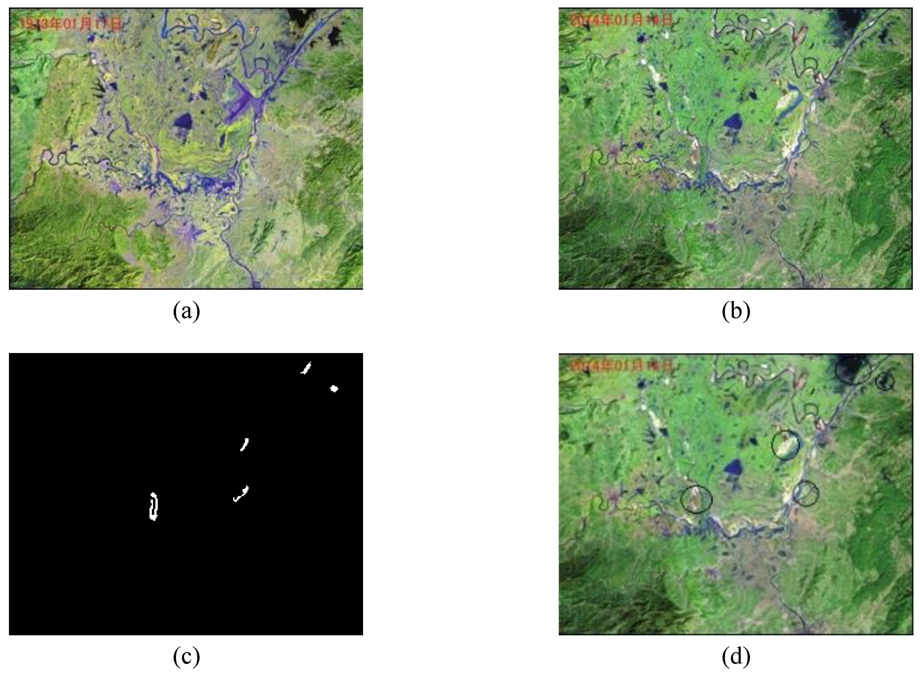
This method can be used to detect and analyze changes in the water environment and provide help for water environment management. We examined the changes in the Dongting Lake in China. The remote sensing images of Dongting Lake from January 1973 and February 2014 are shown in Figure 6a,b. Figure 6a was derived from landsat1 with a resolution of 79 m, while Figure 6b was derived from landsat8 with a resolution of 15 m.

Images collected in the same season can better reflect the real changes in the lake. Figure 6c shows the changes in Dongting Lake on a large scale. The region with the greatest change in the map showed that, after 40 years, the area of some local watersheds had changed, and some local watersheds have changed their original route. Although the results of large-scale detection do not provide specific details, the results can provide location reference for further research.

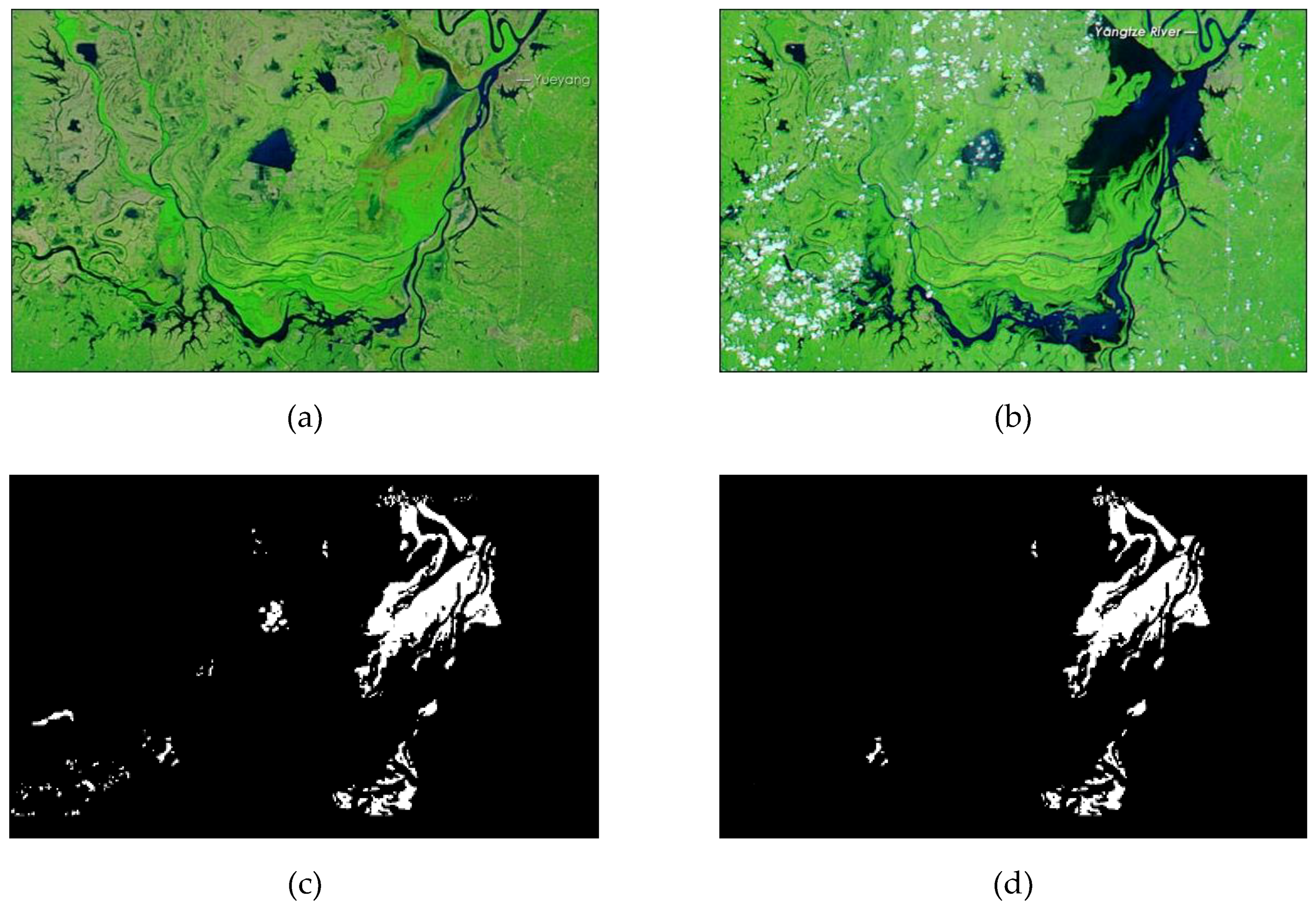
Upon further analysis, changes in the rainy season and dry season in Dongting Lake are shown in Figure 7. The original image size is 4400 × 4000, and the resolution is 10 kilometers [20]. Because of the cloud interference in Figure 7b, the detection result is affected. After removing the cloud and text interference information by color detection [21], the detection result is shown in Figure 7d, and the number of pixels is 8786. The results of change area detection provide a basis for water storage, flood prevention and landform change analysis of Dongting Lake.

6. Conclusions

Addressing the change characteristics of surface types with complex texture information such as rivers and lakes, this paper used an improved directional logarithmic variation function model to analyze the texture features of images and proposes an L-V-NSCT approach. This approach can not only effectively reflect the characteristics of land surface change in different periods but also has good anti-noise performance.

Through our experiments, we can also see that the detection accuracy and other indicators of the proposed method are not stable for different types of images. The stability and parameter settings of the method merit further study.