Vibroacoustic Optimization Study for the Volute Casing of a Centrifugal Fan

Featured Application

Authors are encouraged to provide a concise description of the specific application or a potential application of the work. This section is not mandatory.

Abstract

A numerical optimization is presented to reduce the vibrational noise of a centrifugal fan volute. Minimal vibrational radiated sound power was considered as the aim of the optimization. Three separate parts of volute panel thickness (ST: the side panel thickness; BT: the back panel thickness; FT: the front panel thickness) were taken as the design variables. Then, a vibrational noise optimization control method for the volute casing was proposed that considered the influence of vibroacoustic coupling. The optimization method was mainly divided into three main parts. The first was based on the simulation of unsteady flow to the fan to obtain the vibrational noise source. The second used the design of experiments (DoE) method and a weighted-average surrogate model (radial basis function, or RBF) with three design variables related to the geometries of the three-part volute panel thickness, which was used to provide the basic mathematical model for the optimization of the next part. The third part, implementing the low vibrational noise optimization for the fan volute, applied single-objective (taking volute radiated acoustical power as the objective function) and multi-objective (taking the volute radiated acoustical power and volute total mass as the objective function) methods. In addition, the fan aerodynamic performance, volute casing surface fluctuations, and vibration response were validated by experiments, showing good agreement. The optimization results showed that the vibrational noise optimization method proposed in this study can effectively reduce the vibration noise of the fan, obtaining a maximum value of noise reduction of 7.3 dB. The optimization in this study provides an important technical reference for the design of low vibroacoustic volute centrifugal compressors and fans whose fluids should be strictly kept in the system without any leakage.

1. Introduction

The centrifugal fan is considered a common turbomachinery that is widely used in the ventilation systems of the ship cabin and other sites, bringing comfortable working and living environments for people. However, the noise and vibrations generated with the fan running troubled researchers; thus, the study of the mechanisms of noise and vibration generation and propagation became more and more important. Most of the current studies on fan noise have dealt with aeroacoustic problems. However, the noise is induced not only by internal turbulent flow, but also by flow-induced structure vibration. In some particular application environments, the fluid should be strictly kept within the fan’s systems (e.g., petrochemical compressors and large fans with fan system inlets and outlets are entirely connected to the extended pipe) without any leakage, and the aerodynamic noise-induced unsteady flow of a fan cannot directly spread to the outside. At this moment, the fan casing and the inlet and outlet pipe vibration noise caused by the vibrations of the volute surface are predominant. Therefore, an intensive study of the generation mechanism of the vibrational noise and the noise reduction method is necessary.

In fact, the fan noise induced by unsteady flow belongs to fluid–structure coupling noise, and the impeller and volute can be classified as an elastomer; in particular, the volute vibration cannot be neglected in large fans [1]. In addition, the aeroacoustic and vibroacoustic calculations usually require high computational resources; in order to reduce the computational cost and have an accurate response, hybrid methods are applied. With respect to the vibroacoustics of casings, such as the vibrational noise of car body and compressor casings, the hybrid finite-element method/boundary-element method (FEM/BEM) approach and the hybrid finite-element method/statistical energy analysis (FEM/SEA) approach are often used. It could be also appropriate to cite Citarella and Federico [2], who have made a comprehensive literature review of both the structural and acoustic modeling methods that are used nowadays to predict the vibroacoustics’ performance. They pointed out that lower frequencies, where the tonal resonances are significant, are calculated applying finite element methods (FEM), whereas for higher frequencies, a statistic energy approach can be chosen. Besides, the FEM/BEM method is usually used to perform the free-field sound radiation analysis of open domains. Armentani [3,4] carried out a vibroacoustic analysis for the chain cover of a four-stroke four-cylinder diesel engine through an FEM–BEM coupled approach, while Bianco [5] described an innovative integrated design verification process, based on the bridging between a new semiempirical jet noise model and a hybrid finite-element method/statistical energy analysis (FEM/SEA) approach for calculating the acceleration produced at the payload and equipment level within the structure, vibrating under the external acoustic forcing field. However, there are few studies on the vibration noise induced by the vibration of the casing in a centrifugal fan. This type of noise is prominent in large-scale fan systems and fans with closed pipelines.

At present, research on the vibration noise induced by casing vibration resulting from impeller outlet unsteady flow is usually conducted using simulation methods. A prediction method based on a method of combining boundary element method (BEM) calculations with experimental measurement was proposed by Koopmann [6]. In this method, the aerodynamic noise is isolated, the volute vibrations induced by the unsteady flow are calculated separately, and the pressure fluctuations required for noise and vibration calculations are obtained experimentally. On this basis, some scholars such as Hwang [7], Cai [8,9], and Lu [10] have used the same method to calculate the vibrational sound radiation of a compressor and the T9-19 No.4 industrial centrifugal fan. Cai Jiancheng [11] calculated the vibrational sound radiation of a volute casing of the same centrifugal fan using a fluid–structure–acoustic coupling method. Indeed, this BEM method discretizes the Lighthill equations by applying a free-field Green function integral. At present, the Green function integral method can only solve problems with simple geometric boundaries, and those complex boundaries must be simplified in the free field. Without doubt, this simplification does not consider reflection and scattering effects in the noise propagation. Based on the above advantages, the finite element method (FEM) for solving noise radiation has been recognized by scholars. Durand [12] predicted the structural acoustics of automotive vehicles through using the FEM model. However, there is a computational disadvantage when the finite element method solves the structural acoustic problem of a closed domain. To overcome this disadvantage, automatically matched boundary layers (AMLs) were introduced to simulate the unbound boundary of the exterior computational domain. The outermost layer exposed to the AML surface that satisfied the Sommerfeld radiation condition was defined as a non-reflecting boundary. Based on the FEM method, Zhang [13] performed the aerodynamic noise of the centrifugal fan using the FEM method, and achieved higher prediction accuracy while using less computing resources. To reveal and reduce the noise primarily generated by the freezer fan unit, Onur [14] investigated the vibration and acoustic interactions between the structure and the cavity inside the freezer cabinet, and the FEM method was also used. Zhou [15] performed a vibroacoustic analysis of a centrifugal compressor with connecting piping systems, in which the sound was induced by the unsteady flow in the centrifugal compressor and pipes, and the same FEM method was used. These studies have been of benefit in promoting the development of the research of vibrational sound radiation on structural casing, allowing for a deeper understanding of vibrational noise during the fan operation, and have provided a useful reference for the noise reduction of such machinery.

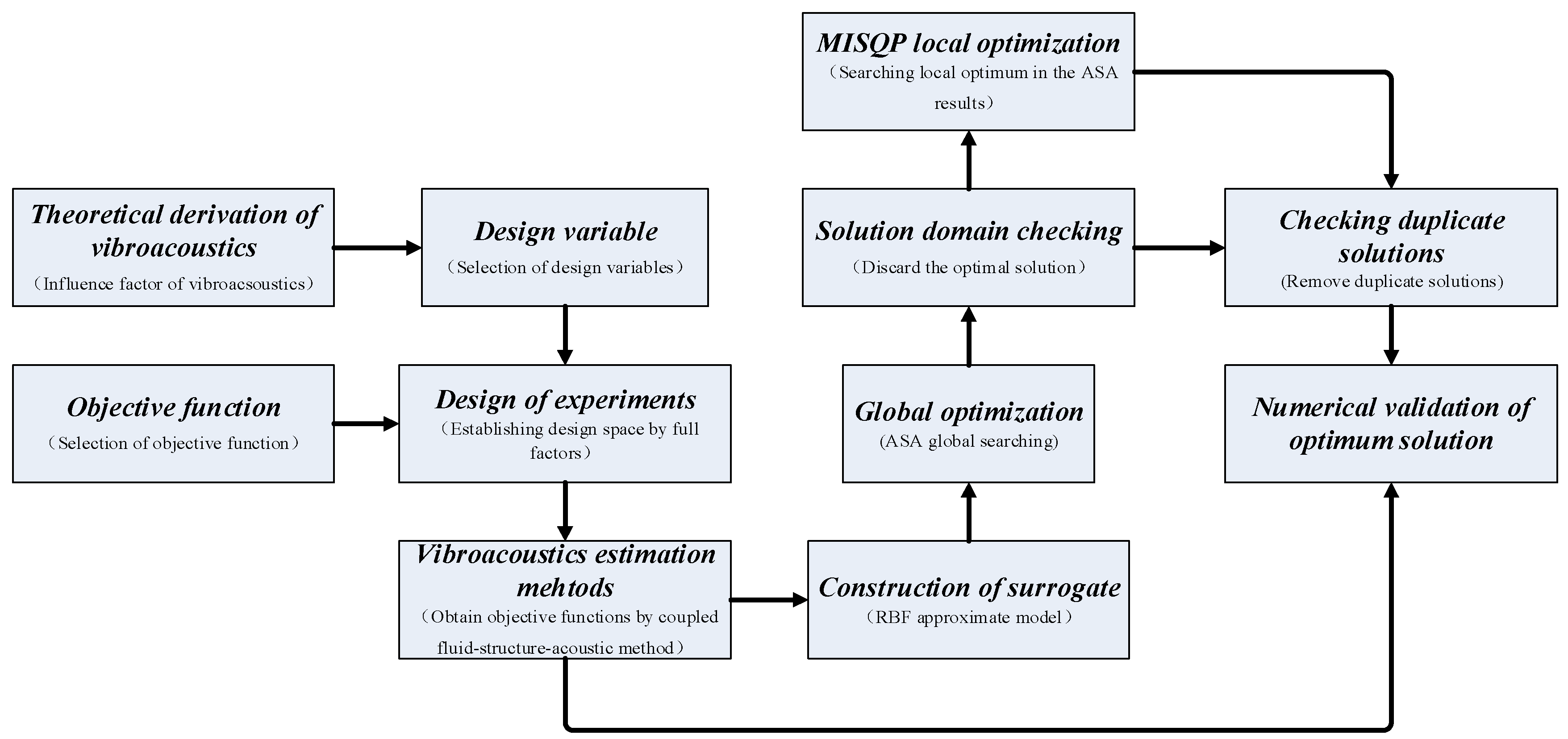
The purpose of vibrational noise research is to explore the generation mechanism of vibrational noise, and then propose targeted methods of vibration and noise reduction. Concerning vibration and noise control, there are certain means: controlling the vibrational source, such as vibration absorption and vibration isolation [16]; dynamic vibration absorption; damping vibration control [17]; and structural vibration control [18,19,20,21,22,23,24,25,26,27]. At present, a structural vibration control method that meets specific requirements by modifying the dynamic characteristics of the controlled object without adding any subsystem is a research hotspot. Moreover, current structural vibration control is focused on structural optimization. However, a centrifugal fan casing belongs to a thin-casing structure, and the vibrational sound power of the thin casing is a quadratic function of the structural vibration velocity [18,19]. As optimization reduces the structural vibration speed of a fan casing, it can be concluded that the sound power radiation must be reduced within a specific range. The optimal design of a thin-casing structure usually uses the panel thickness as the design variable and the square sum of the vibration velocities of the nodes on the wall as the optimization target function [20,21]. Adopting the mentioned method, Zhou et al. [22] and Lu et al. [23] implemented the optimization study on structure vibration control and noise reduction for the T9-19 No.4A centrifugal fan.

By reducing fan casing vibration, an effect of casing noise reduction is achieved using the aforementioned optimization method, which sets the vibration (node vibrational speed) as the target function. However, this method does not consider the propagation of sound waves and sound boundary influences on the calculation results; thus, deviation is nearly inevitable. The integration of structural–acoustic optimization correctly eliminates these drawbacks. This method has been used in the automotive field, and shows that the sound radiation generated by the excitation of body surface vibrations on the engine is substantially reduced [24,25,26,27] after optimization. Based on the aforementioned advantages of optimization, the authors proposed a vibration–acoustic integrated optimization design method that is suitable for turbomachinery volute. In investigating the vibrational noise of the studied marine centrifugal fans, the following three aspects were the focus:

(1) In this study, we proposed a numerical method for one-way fluid–solid–acoustic coupling. The rationality of this one-way coupling is verified by a volute wall vibration test.

(2) To analyze the influence factors of vibrational noise and reduce the vibrational sound radiation induced by unsteady flow in the fan, a detailed theoretical derivation of vibration noise is put forward.

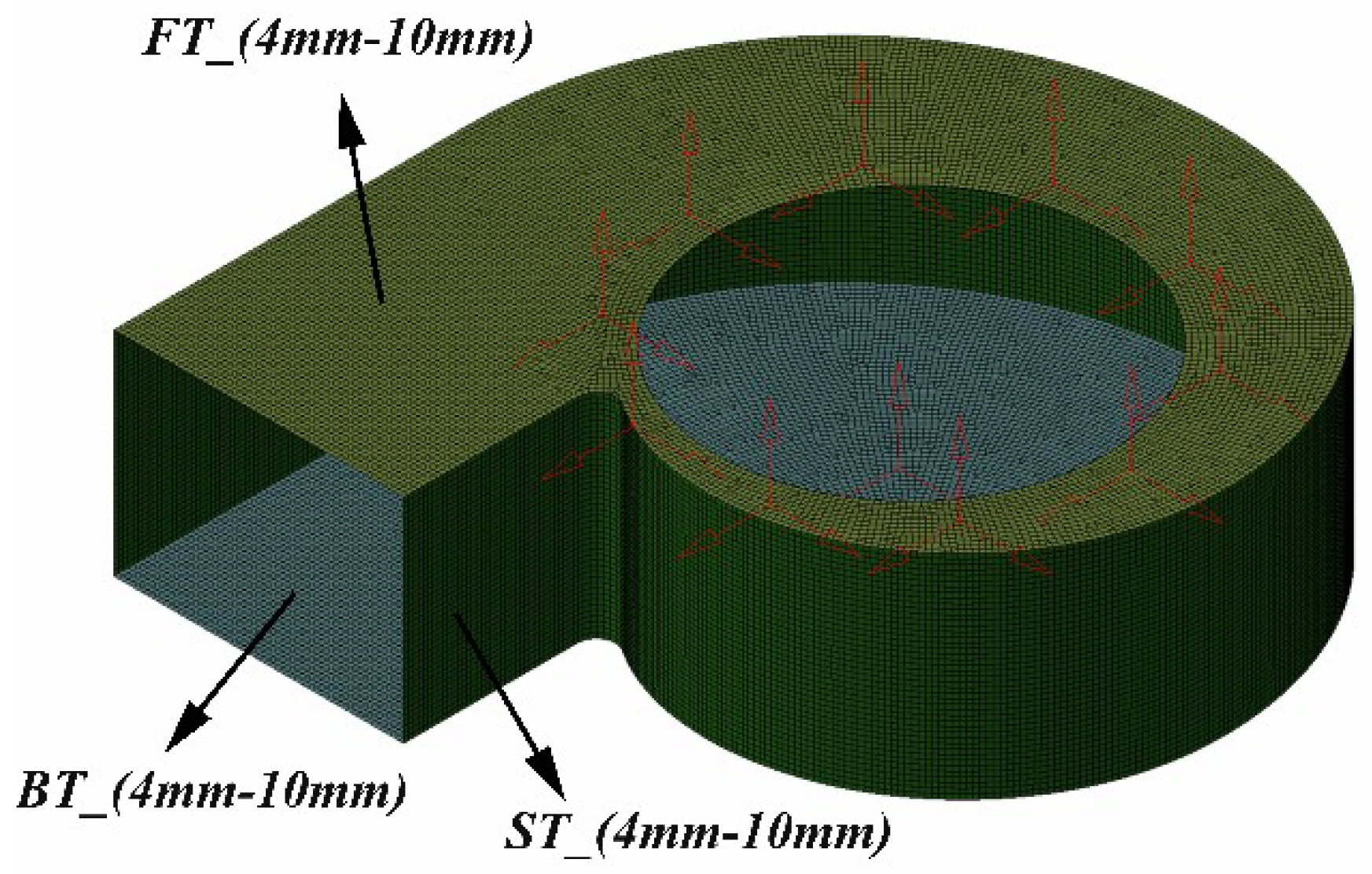
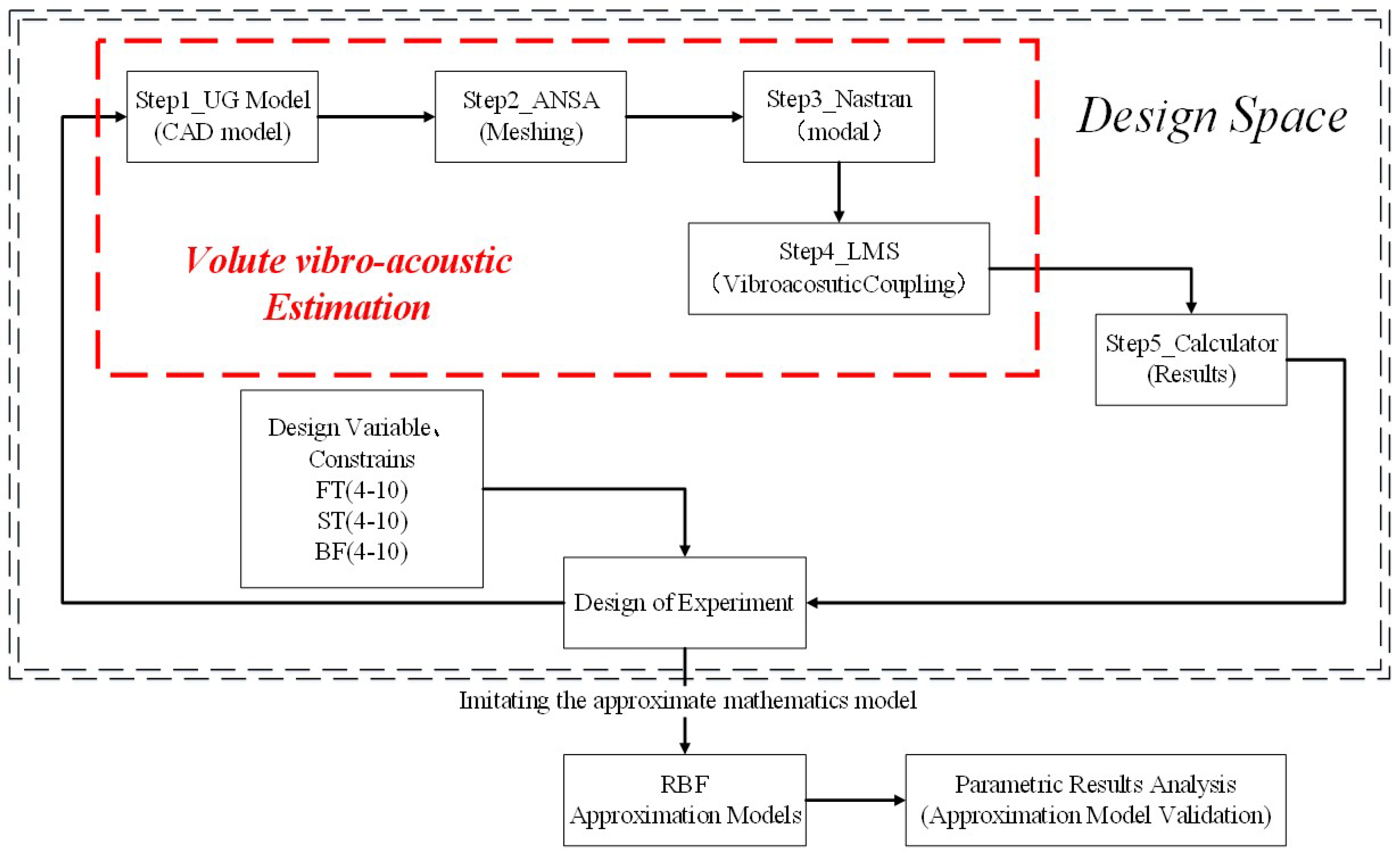
(3) To control the vibrational noise of a certain type of marine centrifugal fan volute, an optimization method considering the influence of vibroacoustic coupling is proposed. Under the premise of whether volute total mass constraints, accordingly taking the panel thickness of the volute casing (FT: the front panel thickness, ST: the side panel thickness, BT: the back panel thickness) as the design variable, this study conducted low vibrational noise single target (taking the volute vibrational radiated sound power as the target function) and multi-target optimization (taking the volute vibrational radiated sound power and total mass as the target function).

2. Centrifugal Fan Description

The studied machine was a ventilating centrifugal fan with four main components (conical bell mouth, shrouded impeller, volute casing with conventional tongue, and conical flow rates throttle) driven by an AC inverter motor with adjustable angular speed between ~0–3600 r/min; the design rotational speed was specified as 2920 r/min, as shown in Figure 1. The main dimensions and characteristics of the investigated fan for this study are presented in

Table 1. Fan dimensions.

Parameters Description	Parameter Values
Impeller blade outlet diameter D2 (mm)	520
Impeller blade inlet diameter D1 (mm)	328
Impeller outlet width b2 (mm)	102
Impeller inlet width b1 (mm)	138
Blade number Zn	12
Volute width B (mm)	286
Impeller-tongue distance (mm)	38
Impeller-tongue distance (% of D2)	13.2%

. The ambient air was intake from the inlet pipe. The tests for characterizing the aerodynamic and acoustic behaviors of the fan system were made in a resilient installation to fulfill ship system noise and vibration requirements (according to standards GJB4058-2000 China [28] and GB-T1236-2000 China [29]). Figure 2a shows the details of the test system installation and data collection procedure. The following maximum measurement errors were obtained for the different magnitudes: total pressure ±2% (±10 Pa), flow rate: ±2% (±0.05 m³/s), and shaft power ±2% (±50 W).

3. Vibroacoustic Aerodynamics

3.1. Numerical Methods

CFD (Computational fluid dynamics) technology has been proven to be a very useful tool in the analysis of the internal flow of turbomachinery both in design and performance prediction. It has been widely applied to simulate the fully three-dimensional (3D) unsteady flow in centrifugal turbomachinery. In this part, the unsteady aerodynamic forces that excite vibrational noise are calculated by CFD. The whole unsteady flow for the entire impeller-volute configuration was conducted using the computational fluid dynamics (CFD) code ANSYS CFX. The numerical simulation is based on a finite-volume numerical method that employs an incompressible flow model to solve the Unsteady Reynolds Averaged Navier–Stokes equations (URANS). The characteristic Mach number of the simulated fan described by the blade tip circumferential velocity was u₂/c = 0.18 (<0.3); therefore, the flow was guaranteed to be incompressible. The continuity equation and momentum equations were solved independently of the energy equation because of the isothermal flow. The standard k-ε turbulence model, which Ballesteros-Tajadura [30] and Cai [31] applied to capture wall pressure fluctuations, was used in the present simulation of the unsteady flow field. A coupled solver, which uses a fully implicit discretization scheme to solve all of the equations (corresponding to the velocity and pressure), was used. However, a second-order high-resolution discretization scheme was used for the convection terms, and a second-order backward Euler scheme was used for the transient terms.

For the three-dimensional calculations, a couple of high-quality hexahedral structural grids were employed to define the flow domains. Details of the grid features and meridian grid cross-section, including the radical gap and cavity around the volute, are shown in Figure 2. More details about the grids of this fan have been reported in the previous work (Jianhua Zhang et al.) [13]. The numerical deviations result from the grid number needed to be removed, and a grid-independent validation of the fan total pressure coefficient and efficiency was performed. Figure 3 shows the influence of the grid size on the fan total pressure coefficient and efficiency. From Figure 3, we can see that the grid was independent when the total number of grid points exceeded 2.8 million. In addition, by increasing the grid size to 5.7 million, the total pressure coefficient with respect to the flow rate was nearly unchanged, compared with the smaller total pressure coefficient over a small flow rate range that was close to the best efficiency point (BEP).

The modeled boundary conditions were considered to have greater physical meaning for turbomachinery flow simulations. In this case, the CFD simulation process began with a steady flow calculation using the frozen-rotor approach, and nonslip conditions were specified at the solid walls. In addition, for the near-wall flow region, a scalable wall function treatment based on the logarithmic law [32] was applied to cause the mean value of y⁺ (y+ is the dimensionless distance from the wall; it is used to check the location of the first node away from a wall) to vary between 30–300 (the recommended values by ANSYS CFD code to ensure a high calculation accuracy), as shown in Figure 4. Therefore, by applying this method, the number of the grid points was greatly reduced without reducing the calculation accuracy. For the unsteady flow, a transient rotor/stator grid interface based on the sliding grid technique was applied, which allowed unsteady interactions between the impeller and volute casing. A time step of 5.7089e⁻⁵ s was used for the calculation of the unsteady interactions, which was sufficient for the dynamic analysis. The time step was related to the rotational speed of the impeller, and the time step was specified such that the impeller rotated once in 360 steps (a blade passage defined 30 steps). The number of iterations was adjusted to reduce the residual below an acceptable value at each time step. At each time step, a reduction of 10⁻⁵ (five orders of magnitude) in the residuals for the given variables in the cells was required. The unsteady simulation was initialized using a steady solution, and over 15 revolutions (approximately 5400 time steps) were required to converge on a periodic unsteady solution.

3.2. CFD Validation

3.2.1. Experiments Description

In this part, the Dynamic Pressure Testing System (DPTS) was employed to obtain the information of the casing pressure fluctuations. This system contained XCQ-080-5G Kulite highfrequency dynamic pressure sensors (Kulite, Leonia, NJ, America), standard power supplies, 8300 AU amplifiers (Econ, Hangzhou, China), and AVANT MI-7016 signal acquisition (Econ, Hangzhou, China). The test system installation is shown in Figure 5. There are 44 measurement locations on the casing surface, which were at five locations (p01–p05) in the vicinity of the volute tongue, and another six monitoring locations (p06–p11) were evenly distributed along the circumferential direction of the volute.

Table 2. Angular coordinate of the measurement points over the volute.

Tongue Points	Angular Position (°)	Volute Points	Angular Position (°)
P1	0	P6	52
P2	3	P7	97
P3	8	P8	142
P4	14	P9	187
P5	20	P10	232
-	-	P11	280

summarizes the angular coordinates of the measurement positions over the volute surface. The locations of monitoring points are shown in Figure 6. The origin of the angle is the volute tongue. At each angular position, four axial measurements were made at the following Z/B coordinates: 0.17, 0.27, 0.34, and 0.75 (B is the volute axial width, and Z is the axial measurement position from the volute rear casing). Z/B = 0.07 corresponds to the impeller hub, and Z/B = 0.36 corresponds to the impeller shroud. More details about the DPTS installation and test have been reported in the previous work (Jianhua Zhang et al.) [13].

3.2.2. Aeodynamic Characteristics Validation

Using the defined test bench, the overall performance of this fan as predicted by the CFD calculations was compared for different flow rates. The non-dimensional flow rate and the total pressure rise were transformed by:

$$\phi =\frac{4Q}{D_2^2{u}_2\pi }$$

(1)

$$\psi =\frac{P_T}{\rho u_2^2}$$

(2)

The best efficiency point (BEP) at a rotational speed 2920 rpm corresponded to a flow rate Q = 3.3614 kg/s (φ = 0.1659) and a total pressure rise P_T = 3182 Pa (ψ = 0.41954). Figure 7 indicates that the measured total pressure coefficient and efficiency agreed well with the three-dimensional steady-state calculations. The expected trend of decreasing total pressure coefficients with increasing flow rates can be observed in the experimental and numerical curves. In addition, the performance curves between the numerical simulation and experimental test results were perfectly consistent regards of larger grids (nearly double the size of the small grids).

3.2.3. Unsteady Pressure Fluctuation Validation

The pressure fluctuations on the volute casing induced by the unsteady flow at the impeller outlet are the significant vibration noise sources; thus, the validation of the unsteady aerodynamics is very important. In this study, to confirm the simulation accuracy, a comparison analysis between the dynamic pressure measurement results of volute casing and the numerical calculation was conducted. Due to the similar spectrum signals of the different measurement points on the volute surface, only a few typical points were selected for analysis and confirmation. Figure 8 shows the power spectrum of the volute pressure fluctuations at the BEP at the typical selected measurement points: point 01, point 06, and point 09. The left figure shows the experimental measurement results, and the right figure shows the numerical results. It can be found that the numerical and experimental amplitude of the blade-passing frequency (BPF), which presented the predominant frequency component, were in good agreement at the three most important axial positions (Z/B = 0.17, 0.27, and 0.34). More details about the results discussion have been reported in the previous work (Jianhua Zhang et al.) [13].

4. Volute Vibroacoustic Model, FEM Validation, and Simulation

For the simulated fan, the displacement of the volute vibration was very small, and the flow was incompressible. Furthermore, the characteristic Mach number was smaller than 0.3. Therefore, the volute’s vibration influence on the internal flow was neglected. Therefore, one-way fluid–solid coupling was applied in the simulation. Jiang et al. [33] applied a one-way coupling technique that validated the rationality of an unsteady flow-induced vibration of a centrifugal pump. The validation of one-way coupling is also presented in this study. For details, please refer to Section 4.2.

4.1. Vibroacoustic Mathematical Model

For a continuous system of an actual structure, which was dispersed by FEM, the dynamic balance equation is as follows:

$$M\ddot{x}\left(t\right)+C\dot{x}\left(t\right)+kx\left(t\right)=\mathit{F}\left(t\right)$$

(3)

As the structure is subjected to external harmonic force, the external force can be expressed as follows:

$$\mathit{F}(t)=\mathit{F}\cdot e^{jwt}$$

(4)

The modal vectors are linearly independent of each other. Therefore, the response of the dynamic under any excitation can be regarded as the coupling of the systematic modes and the modal participation factors (MPFs) of each order. At this point, the displacement response can be expressed as follows:

$$x(t)={\displaystyle \sum _{i=1}^n{\mathsf{\phi }}_i{y}_i\left(t\right)}=\Phi Y$$

(5)

In the formula, ${\phi }_i$ represents the ith mode shape of the structure, and $y_i\left(t\right)$ represents the ith mode coordinate, which is called the ith MPFs; $\Phi =\left[{\mathsf{\phi }}_1{\mathsf{\phi }}_2\cdot \cdot \cdot {\mathsf{\phi }}_n\right]$; $Y=\left[y_1{y}_2\cdot \cdot \cdot y_n\right]$. Substituting Equation (5) into Equation (3) and multiplying ${\Phi }^T$ on the two laterals yields the following:

$${\Phi }^{T}M\Phi \ddot{Y}+{\Phi }^{T}C\Phi \dot{Y}+{\Phi }^{T}K\Phi Y={\Phi }^T\mathit{F}{\mathrm{e}}^{j\omega t}$$

(6)

Using the orthogonality of the modal vectors for the mass, damping, and stiffness matrixes, we obtain independent coefficients of the single degrees of freedom of n items. Therefore, the original system can be regarded as linear superposition independent coefficients of single degrees of freedom of n items.

If,

$${\Phi }^{T}M\Phi =m_i,{\Phi }^{T}C\Phi =C_i,{\Phi }^{T}K\Phi =K_i,{\Phi }^T\mathit{F}={\mathit{F}}_i$$

(7)

Then, substituting Equation (7) into Equation (6), the transformation is as follows:

$$m_i{\ddot{y}}_i(t)+C_i{\dot{y}}_i(t)+K_i{y}_i(t)=F_i{e}^{j\omega t}$$

(8)

If,

$${\omega }_n=\sqrt{\frac{k_i}{m_i}},{\zeta }_i=\frac{c_i}{2\sqrt{k_i{m}_i}}$$

(9)

Then, substituting Equation (9) into Equation (8) results in the following:

$${\ddot{y}}_i(t)+2{\zeta }_i{\omega }_n{\dot{y}}_i(t)+{\omega }_n^2{y}_i(t)=F_i{e}^{j\omega t}$$

(10)

Using the theory of ordinary differential equations, we obtain the stable solution of Equation (4) as follows:

$$y_i(t)=\frac{F_i}{{\omega }_n^2-{\omega }^2+2j{\zeta }_i\omega {\omega }_n}{e}^{j\omega t}$$

(11)

Introducing the frequency ratio $\mathsf{\lambda }={\omega }_n/\omega$ and the dimensionless vibration mode amplification factor ${\beta }_i$ results in the following:

$${\beta }_i=\frac{1}{\sqrt{{({\lambda }^2-1)}^2+{(2{\zeta }_i\lambda )}^2}}$$

(12)

Ordering:

$${\psi }_i=\arctan \frac{2{\zeta }_i\lambda }{{\lambda }^2-1}$$

(13)

Substituting equations (12) and (13) into Equation (11) results in the following:

$$y_i(t)=\frac{F_i}{{\omega }^2}{\beta }_i{e}^{j(\omega t-\psi )}$$

(14)

At this point, the vibrational displacement is as follows:

$$\mathit{x}(t)={\displaystyle \sum _{i=1}^n{\mathsf{\phi }}_i{y}_i\left(t\right)}={\displaystyle \sum _{i=1}^n{\mathsf{\phi }}_i\frac{F_i}{{\omega }^2}{\beta }_i{e}^{j(\omega t-\psi )}}$$

(15)

The vibrational velocity is as follows:

$$\dot{\mathit{x}}(t)={\displaystyle \sum _{i=1}^n{\mathsf{\phi }}_i{\dot{y}}_i\left(t\right)}={\displaystyle \sum _{i=1}^n{\mathsf{\phi }}_i\frac{F_i}{\omega }{\beta }_i{e}^{j(\omega t-\psi +\frac{\pi }{2})}}$$

(16)

The active output power is as follows:

$$W_{o,active}={\displaystyle \underset{S}{\int }\mathrm{Re}(I_n)}ds=\frac{1}{2}{\displaystyle \underset{S}{\int }\mathrm{Re}(p{v}_n^{*})}ds$$

(17)

The relationship between the plane wave sound pressure p and the surface velocity $v_n^{*}$ is as follows:

$$p={\rho }_0{c}_0{v}_n^{\ast }$$

(18)

Substituting Equation (18) into Equation (17) results in the following:

$$W_{o,active}={\displaystyle \underset{S}{\int }\mathrm{Re}(I_n)}ds=\frac{1}{2}{\rho }_0{c}_0{\displaystyle \underset{S}{\int }\mathrm{Re}(v_n^{\ast }{}^2)}ds$$

(19)

Substituting Equation (16) into Equation (19) results in the following:

$$W_{o,active}={\displaystyle \underset{S}{\int }\mathrm{Re}(I_n)}ds=\frac{1}{2}{\rho }_0{c}_0{\displaystyle \underset{S}{\int }\mathrm{Re}{({\displaystyle \sum _{i=1}^n{\mathsf{\phi }}_i\frac{F_i}{\omega }{\beta }_i{e}^{j(\omega t-\psi +\frac{\pi }{2})}})}^2}ds$$

(20)

According to Equation (20), it can be concluded that the structural acoustic radiation power is mainly determined by the modal shape ${\phi }_i$, the applied exciting force ${\mathrm{F}}_i$, and the frequency amplification factor ${\mathsf{\beta }}_{\mathrm{i}}$. Therefore, the following methods can be used to control vibrational noise:

(1) With the structural model and material determined, the vibrational sound radiation can be weakened by attenuating the amplitude of the applied exciting force;

(2) With the determination of the exciting force, the geometric parameters of the structural model are modified to reduce the modal shape;

(3) To reduce the amplitude amplification factor, the natural frequency and the external excitation force frequency should be avoided.

Regarding the studied fan volute structure, the structural mode can be changed by controlling the thickness distribution of the structure if the geometry, the stiffness, and the constraint position are all fixed.

4.2. Volute Vibration Simulation and Validation

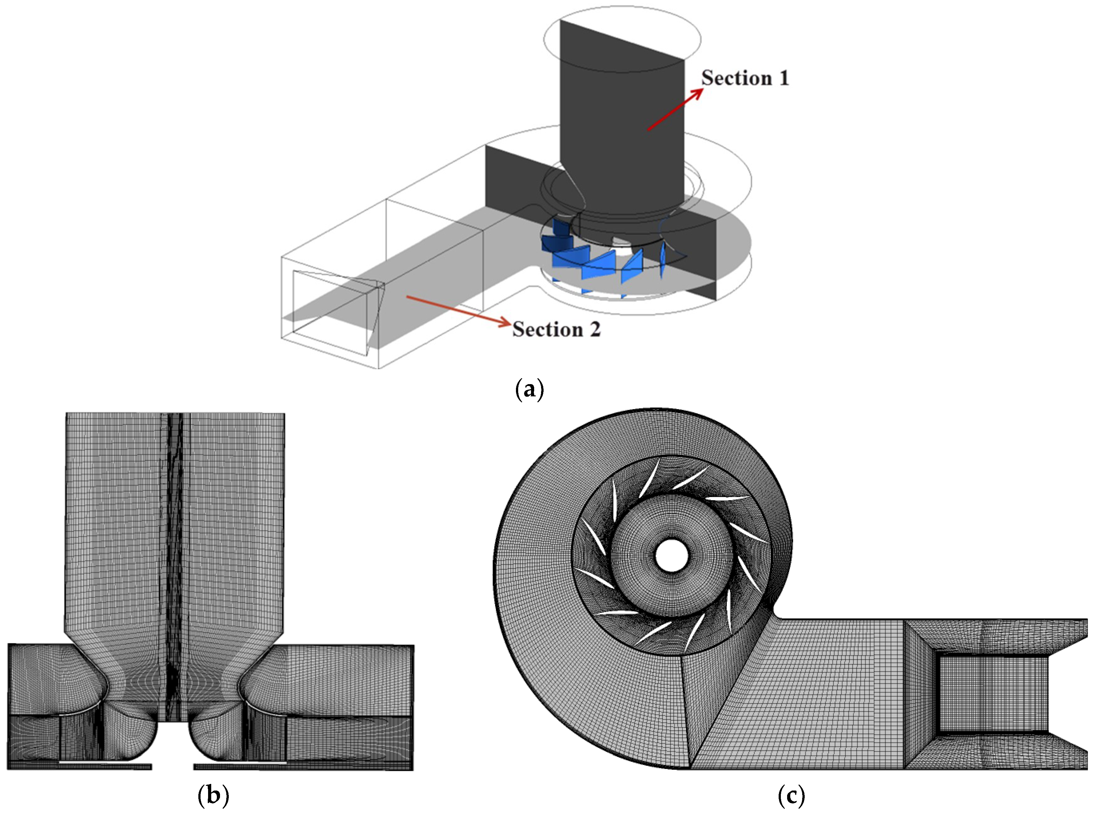
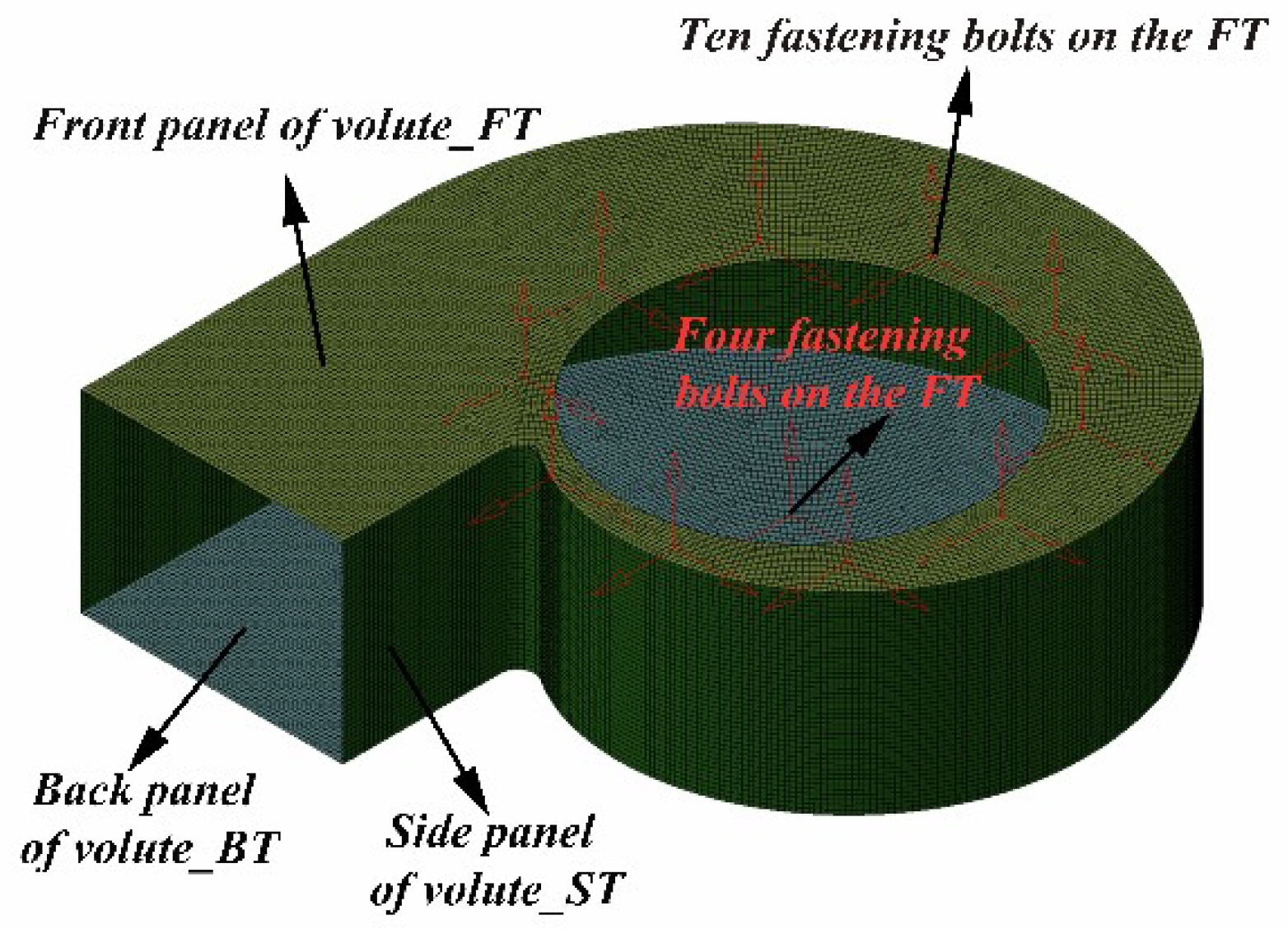
The finite element analysis method is one of the important methods to obtain the vibrations of the structure surface. In this study, N × Nastran, the commercial software made by the Siemens Company, was used to calculate the modal and vibration response of the volute. The finite element model (FEM) of the volute was selected by using a high-quality surface quadrilateral mesh, as shown in Figure 9. The thickness of the volute panel is relatively small (up to six mm), and the shell63 element is selected for the FEM, as the shell63 element has both bending and membrane capabilities, and can suffer from both plane and normal loads. The volute FEM with a total of 46,182 shell63 element grids was divided into three main sections according to the different thickness properties. The front panel thickness (FT) and the back panel thickness (BF) were set to six mm, and the volute side panel thickness was set to five mm (ST). 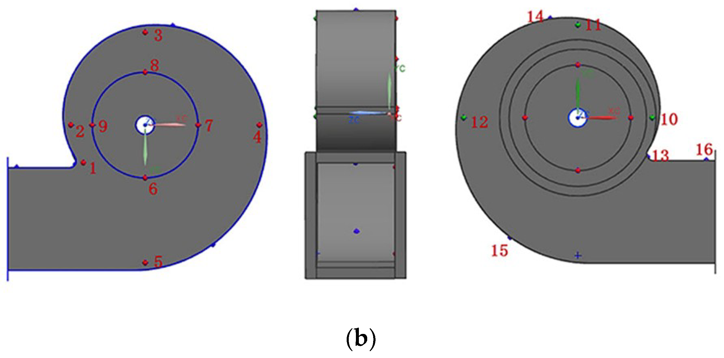In addition, the model material was steel, the density ρ = 7800 kg/m³, the elastic modulus = 2.06e11 pa, and Poisson’s ratio υ = 0.3. The volute casing was fixed to a supporting stand by 10 fastening bolts at the casing front. The volute panel rear (near the motor) was connected by four fixed bolts, and the three translational degrees of freedom of the nodes at the bolts were restricted to zero. The panel thickness distribution and the degree of freedom constraints on the volutes are shown in Figure 9.

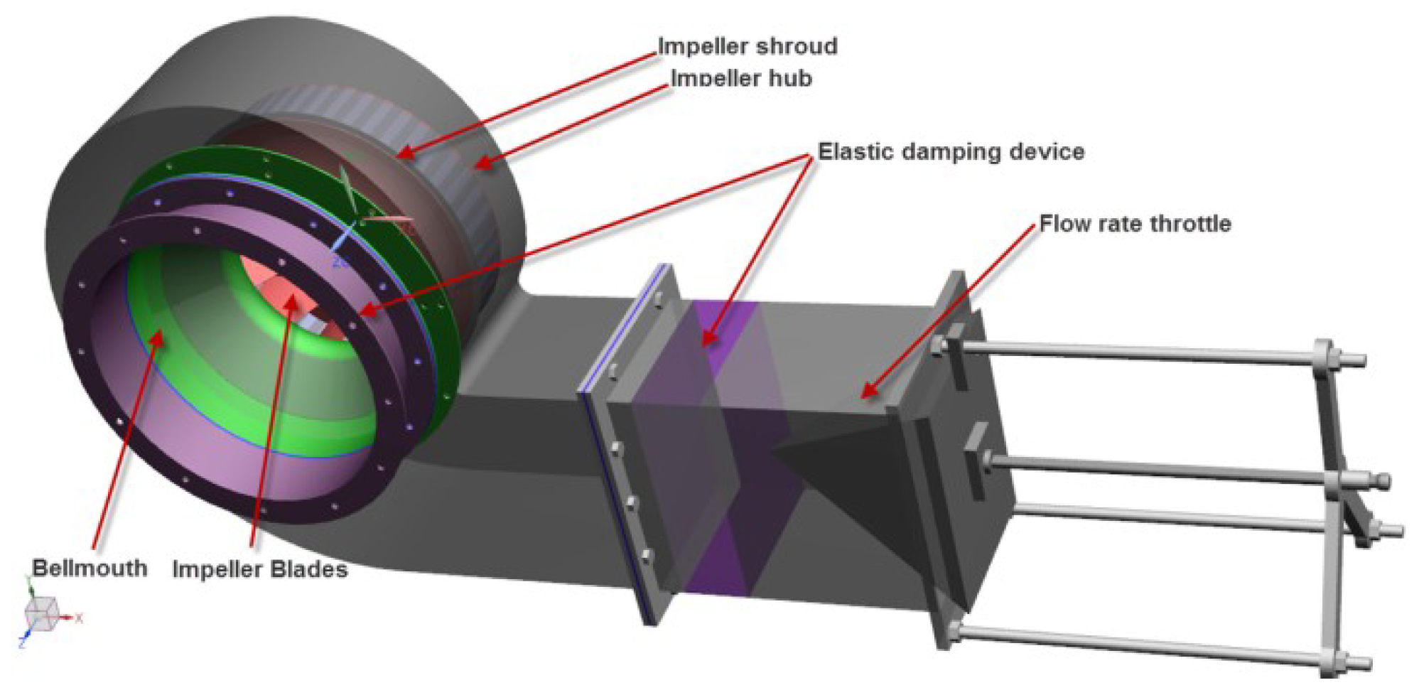
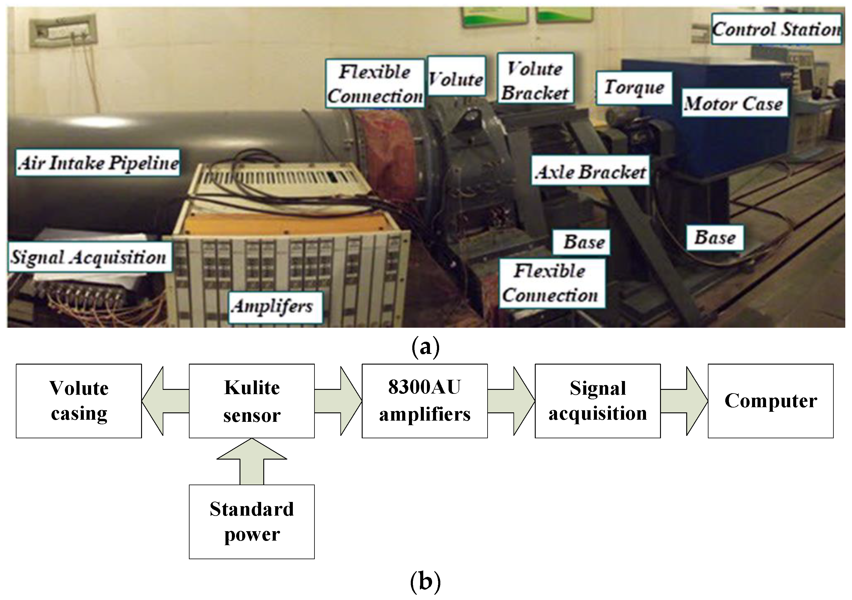
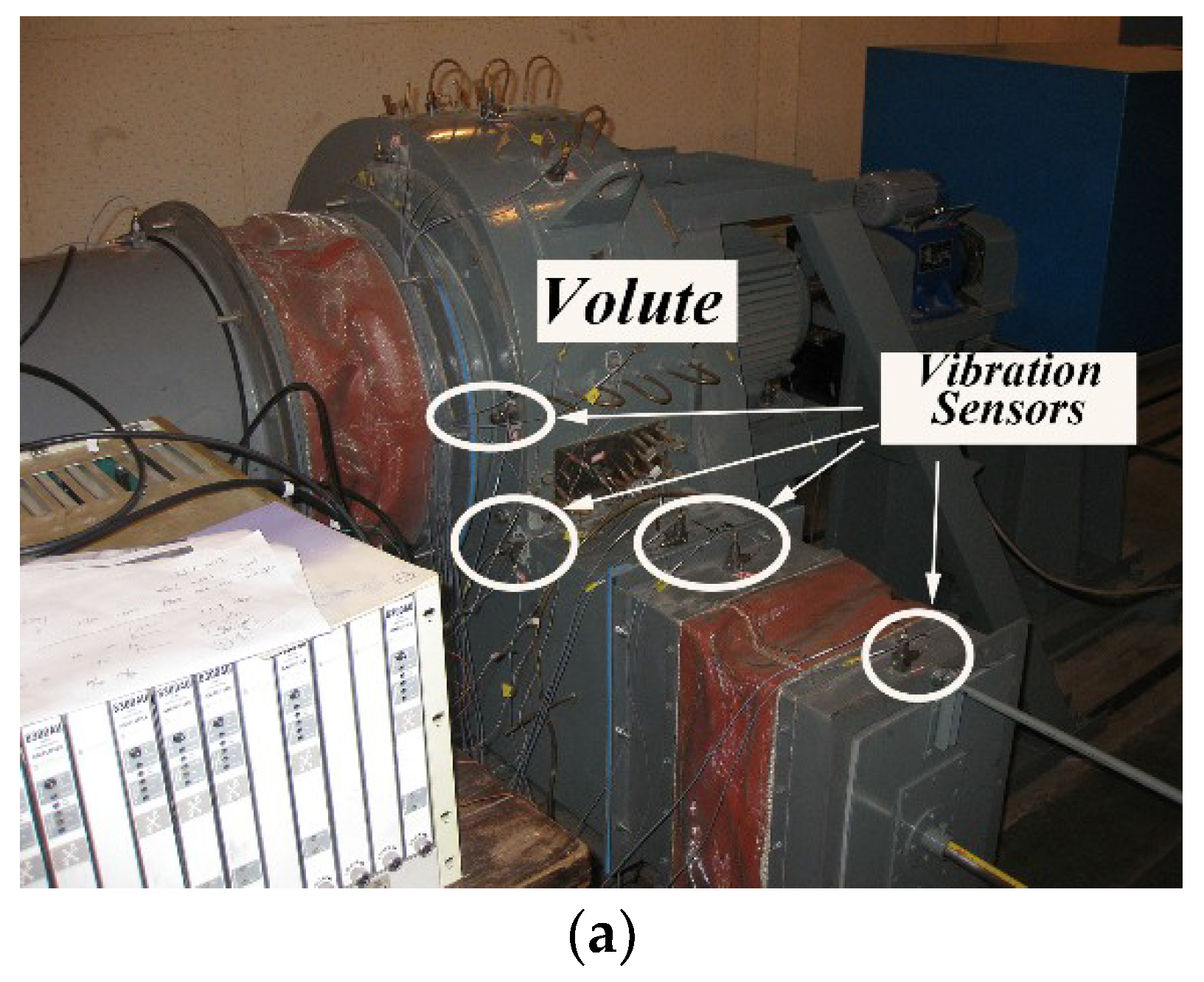
To validate the one-way fluid–solid coupling, vibration analysis was performed, and the results were compared with those of experimental vibrational analysis. The LMS Test Lab test system was used to complete the vibrational test of the fan casing. To eliminate the vibrational disturbances on the volute originating from the imported pipe and outlet throttle flow, elastic connections were used in two positions: at the connection between the transition section of an inlet and the volute, and between the volute outlet and the throttle valve. The flexible installation should meet the requirements of GJB4058-2000 (The Noise and Vibration Measurement Method of Ship Equipment) [28]. There is some major equipment required for this test, such as an LMS SC310W signal analyzer, a B&K 4513 accelerometer, and a B&K 4514 accelerometer. The background noise is ignored because of the lower value compared to the actual value of the fan. One hand of the accelerometer is fixed on the volute by bonding, and the other hand is directly connected to the data processing and analysis notebook by the data line. 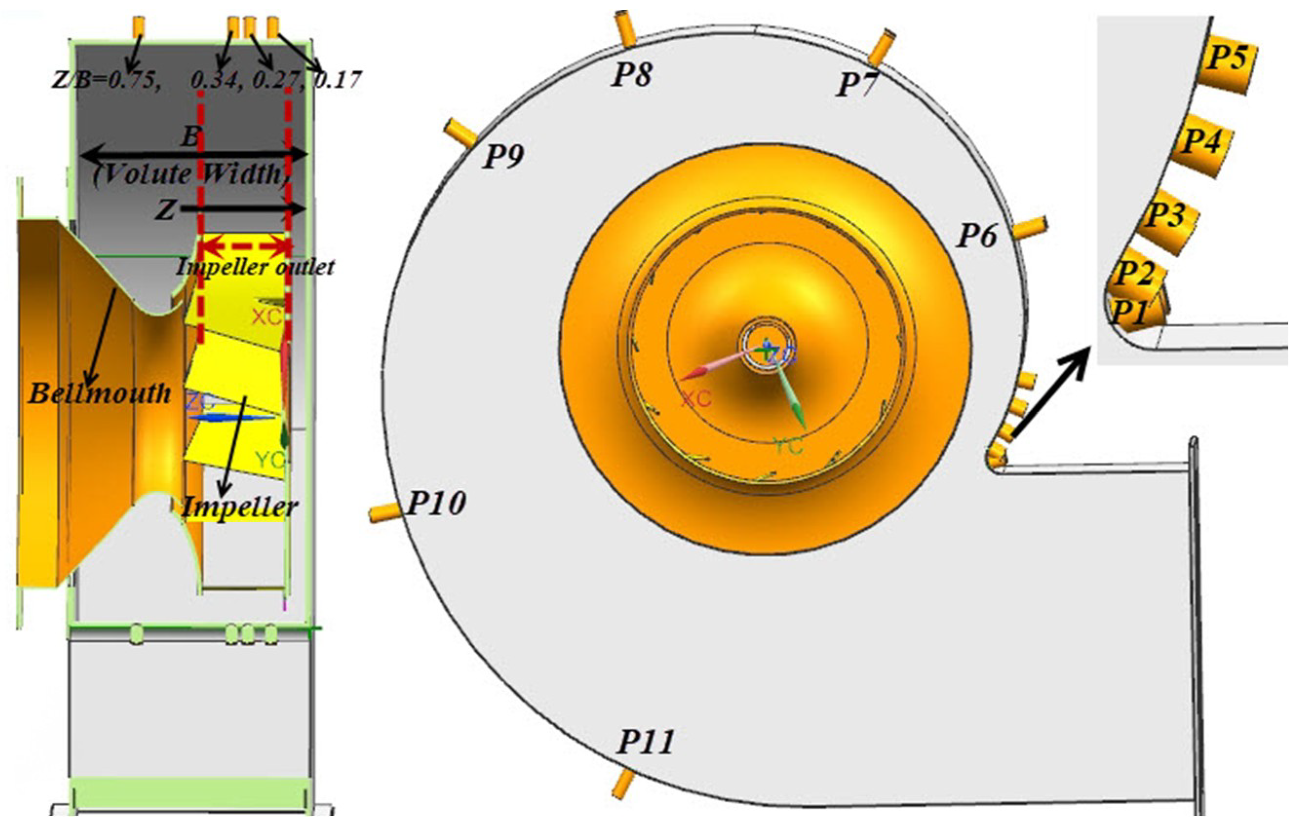The arrangement of the vibration sensor is shown in Figure 10. There are 16 vibration measurement locations on the casing surface. The first five measuring points are arranged near the border between the back panel of the volute and the side panel of the volute. The first measuring point is located near the tongue, and the second through fifth measuring points, #2–5, are respectively arranged at the positions of 0°, 90°, 180°, and 270°. The sixth to ninth measuring points, which are located at the edge of the plate between the back panel of the volute and the motor along with the connecting plate in the circumferential direction, are arranged at an interval of 90 degrees. At the front panel of the volute, with a 90-degree interval in the direction of a counterclockwise rotation layout, are measuring points 10 to 12. The vibration measuring point of the volute side panel is in the middle of the axial width of the volute arranging measuring points 13 to 15. Measuring point 13 is defined as the starting point; measuring points 14 and 15 are also arranged in the side volute at an interval of 140 degrees; and the measuring point 16 is at the outlet of the volute side panel. The vibration test and the dynamic pressure test of the volute are carried out at the same time, and the data are, respectively, collected in different control computers. Then, the data are sequentially extracted to complete the post-processing.

The definition of the total vibrational amplitude is shown as follows:

$$VAL=\sqrt{{\displaystyle \sum _{i=1}^n{a}_{fei}^2}}$$

(21)

where, $a_{fei}$ represents the vibration acceleration at any frequency in the spectrum.

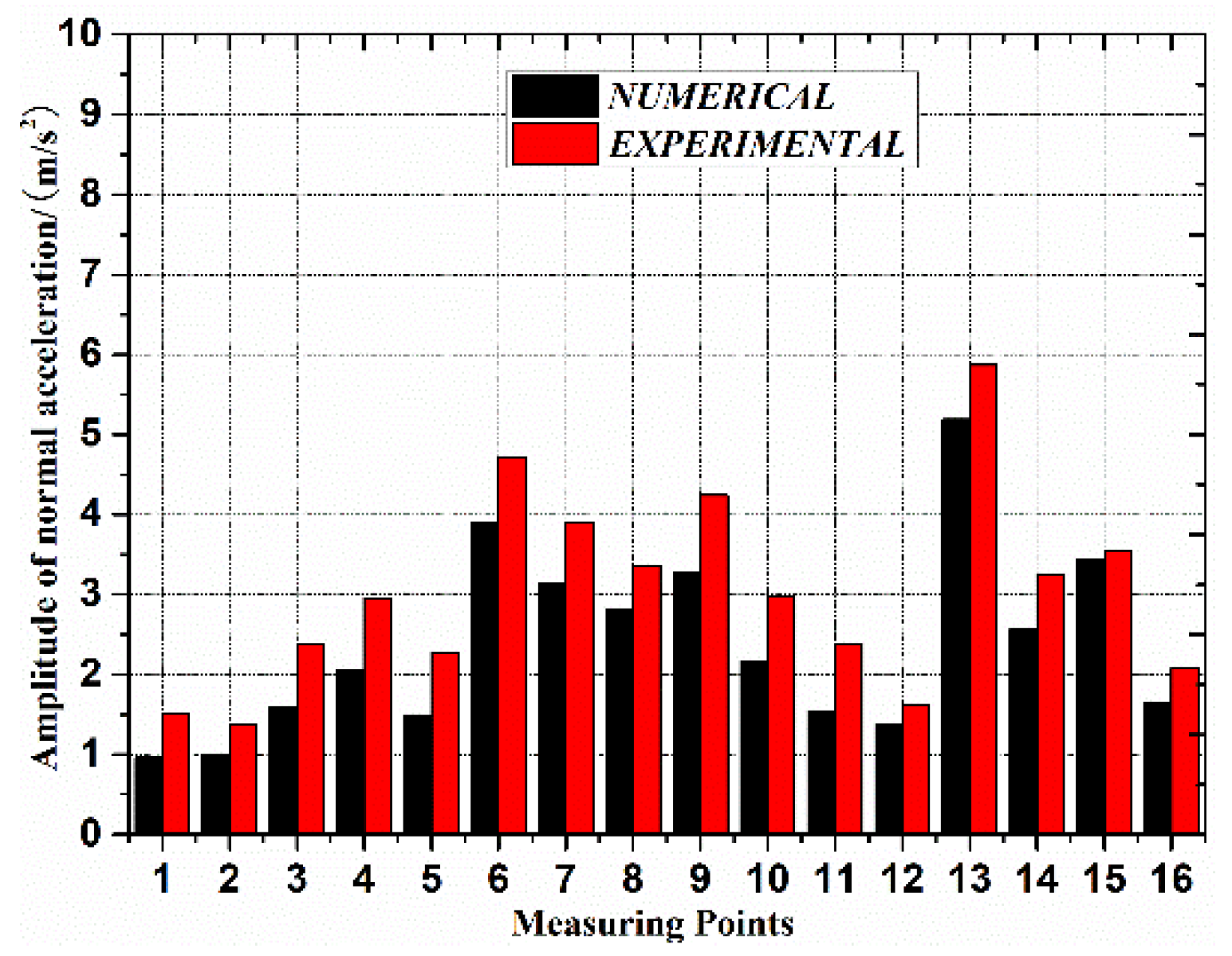
Figure 11 shows a comparison of the numerical and experimental results of the total vibration levels of various vibrational positions in the range of 20 to 3000 Hz. The calculated vibrational measurement positions are arranged according to the vibrational test. Most importantly, it should be stated that the volute casing vibration measurements, the vibration response calculation, and the vibrational noise production are all carried out on the fan design flow rate, the best efficiency point (BEP). As seen in the Figure 11, the calculations are in good agreement with the experiments; the detailed results and analysis refer to the reference [34]. Moreover, a comparison between the experimental and the numerical results shows that it is reasonable and effective to adopt the one-way fluid–structure–acoustic coupling method. 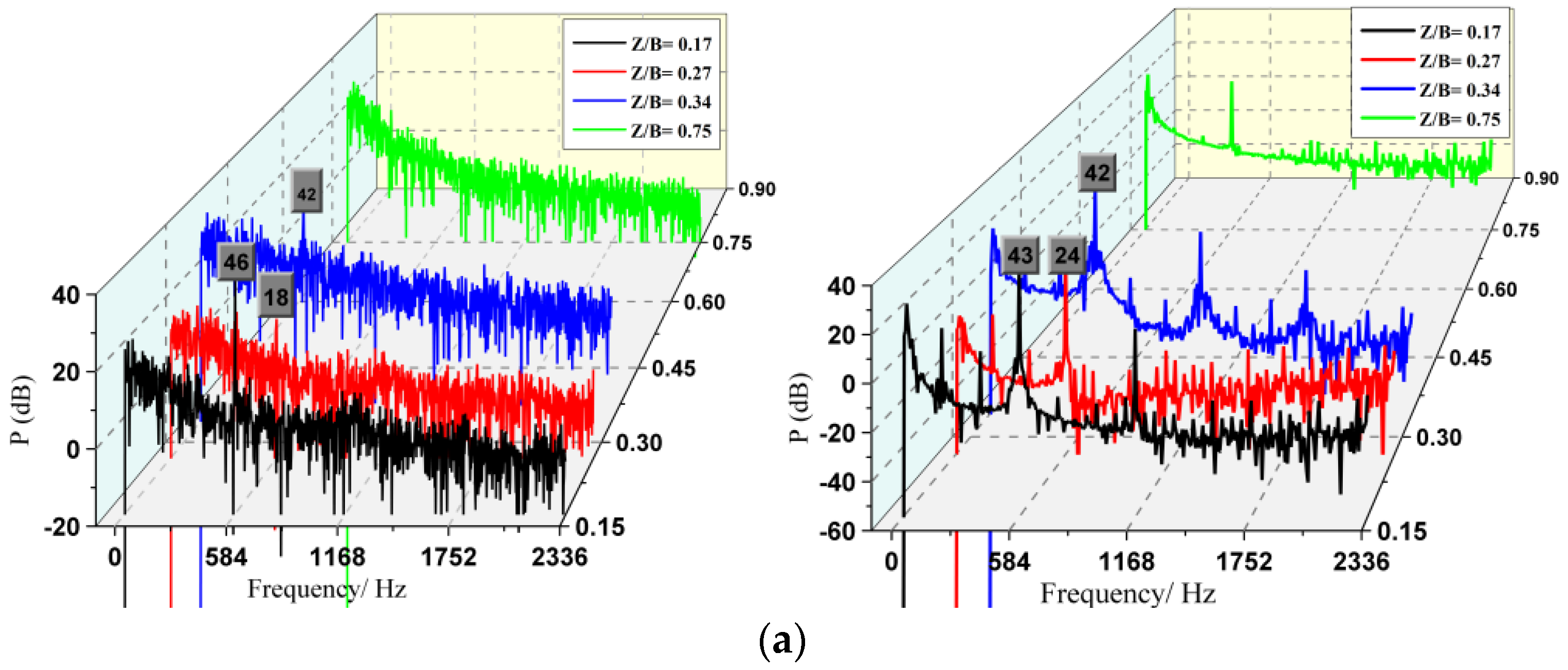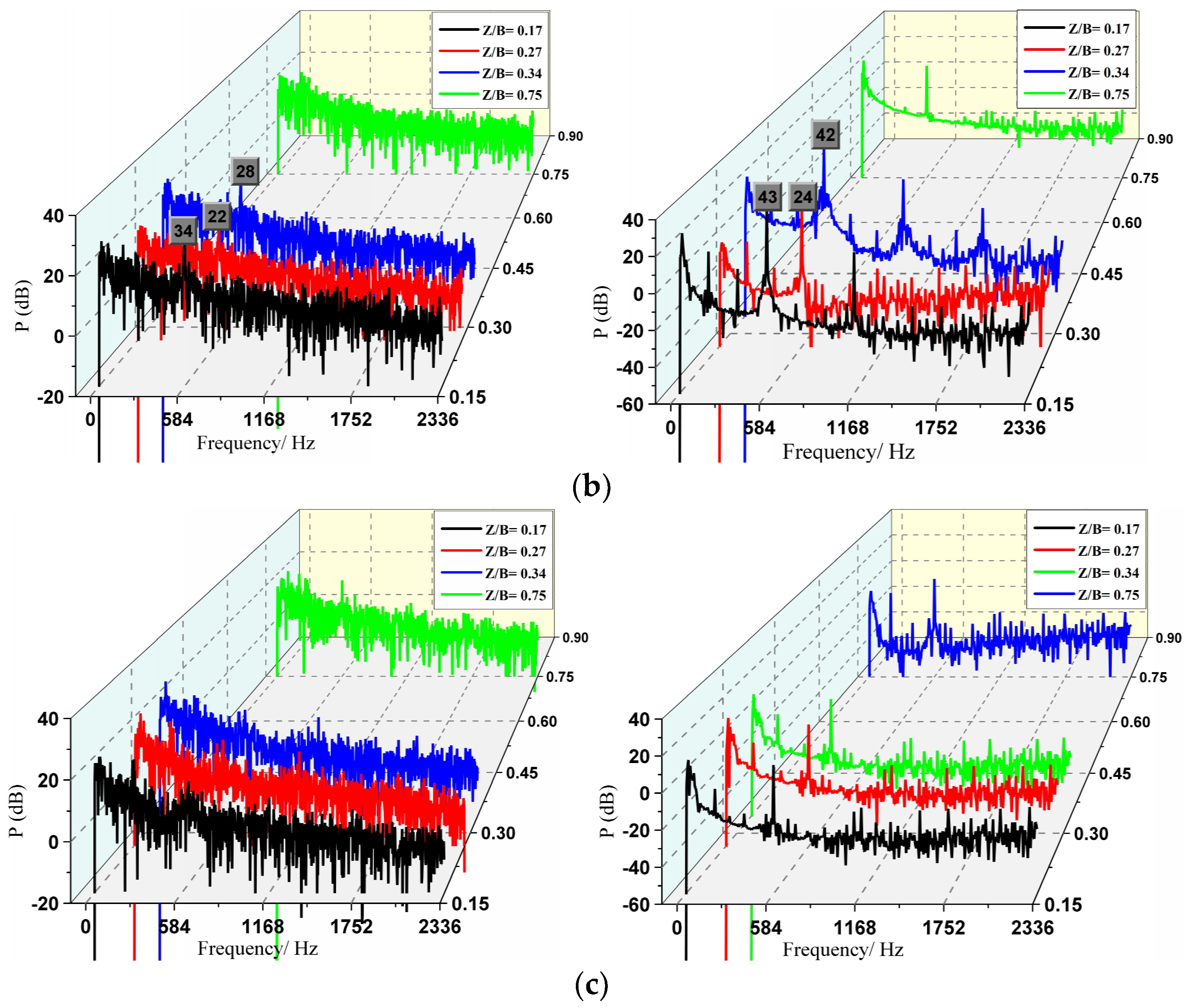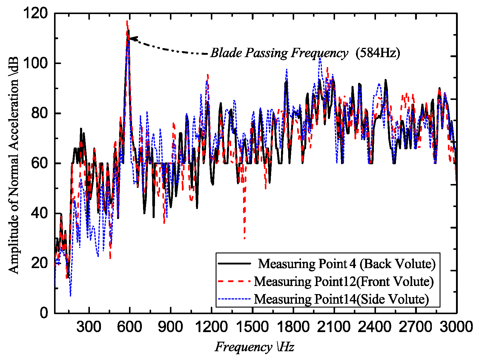Figure 12 presents the vibration acceleration spectrum of the selected three measuring positions (corresponding to the volute rear panel [BT], the volute front panel [FT], and the volute side panel [ST]). It can be seen from Figure 12 that the spectrum waveforms at each measuring position are similar, and the maximum amplitude of vibration acceleration presents at the fundamental frequency, indicating that the fundamental frequency, the blade-passing frequency (BPF), is the major component for volute vibrations induced by unsteady flow.

4.3. Volute Vibroacoustics Estimation Method

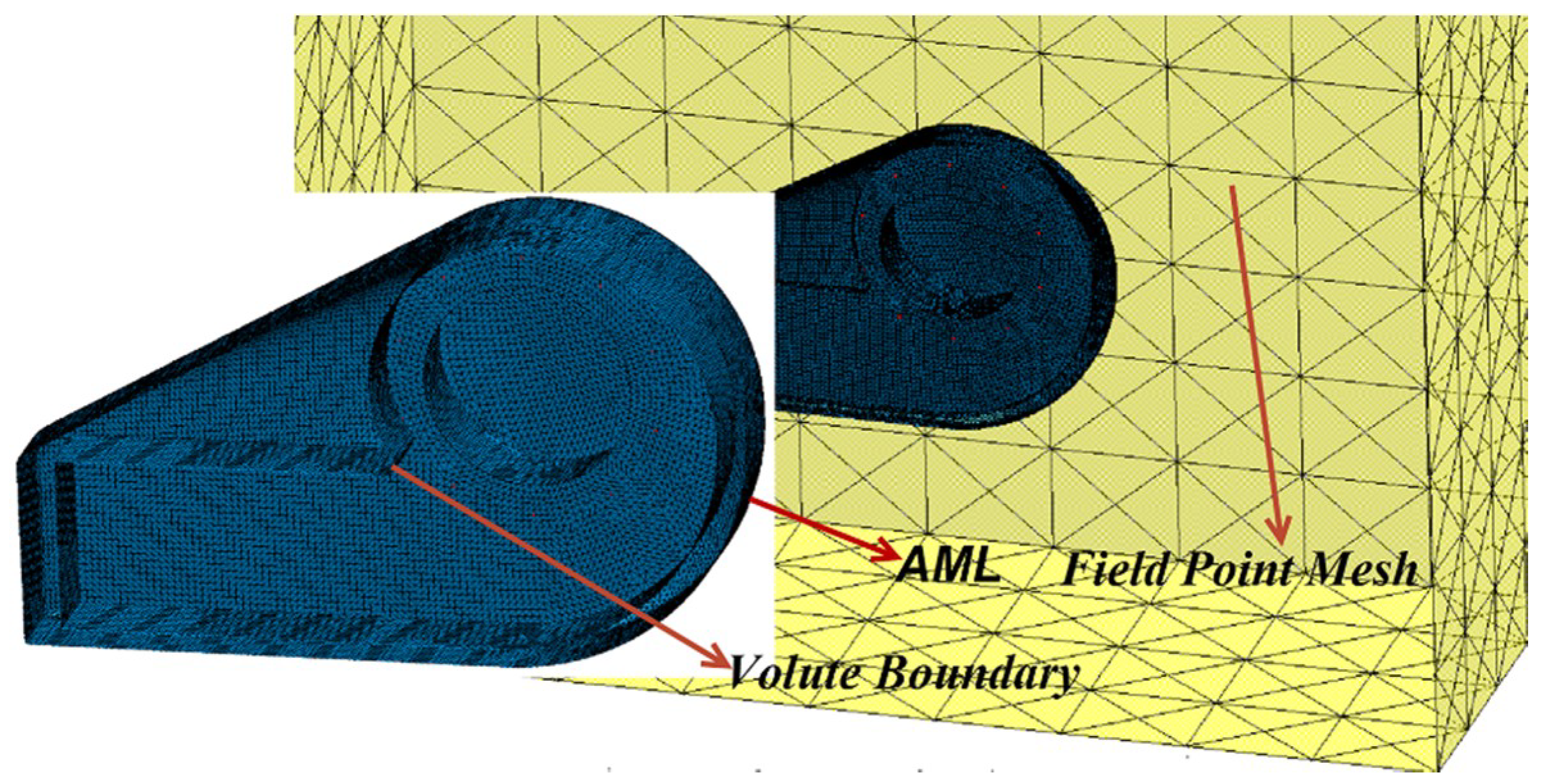
The vibroacoustic simulation was performed using the LMS Virtual Acoustics commercial code, and the volute acoustical FEM model is shown in Figure 13. It was similar to the acoustical finite element mesh that was used for aerodynamic noise calculations [13]. Taking into account the characteristic of radiated vibrational noise, the volute’s inlet and outlet were completely enclosed. More importantly, according to the requirements on element size driven by maximum frequency, the computational acoustic mesh had to satisfy each wavelength corresponding to six elements. An acoustical mesh with a maximum element size of 15 mm was applied in the sound computation, and guaranteed a spatial resolution at the maximum frequency of 3236 Hz of six points per wavelength. Atmospheric boundary layers (AMLs) were introduced to simulate the unbound boundary of the exterior fluid domain. The outermost layer exposed to the AML surface that satisfied the Sommerfeld radiation condition was defined as a non-reflecting boundary. Then, a field point mesh based on standard ISO3744 [35] that enclosed the entire calculation domain was established using an approximate free-field engineering method.

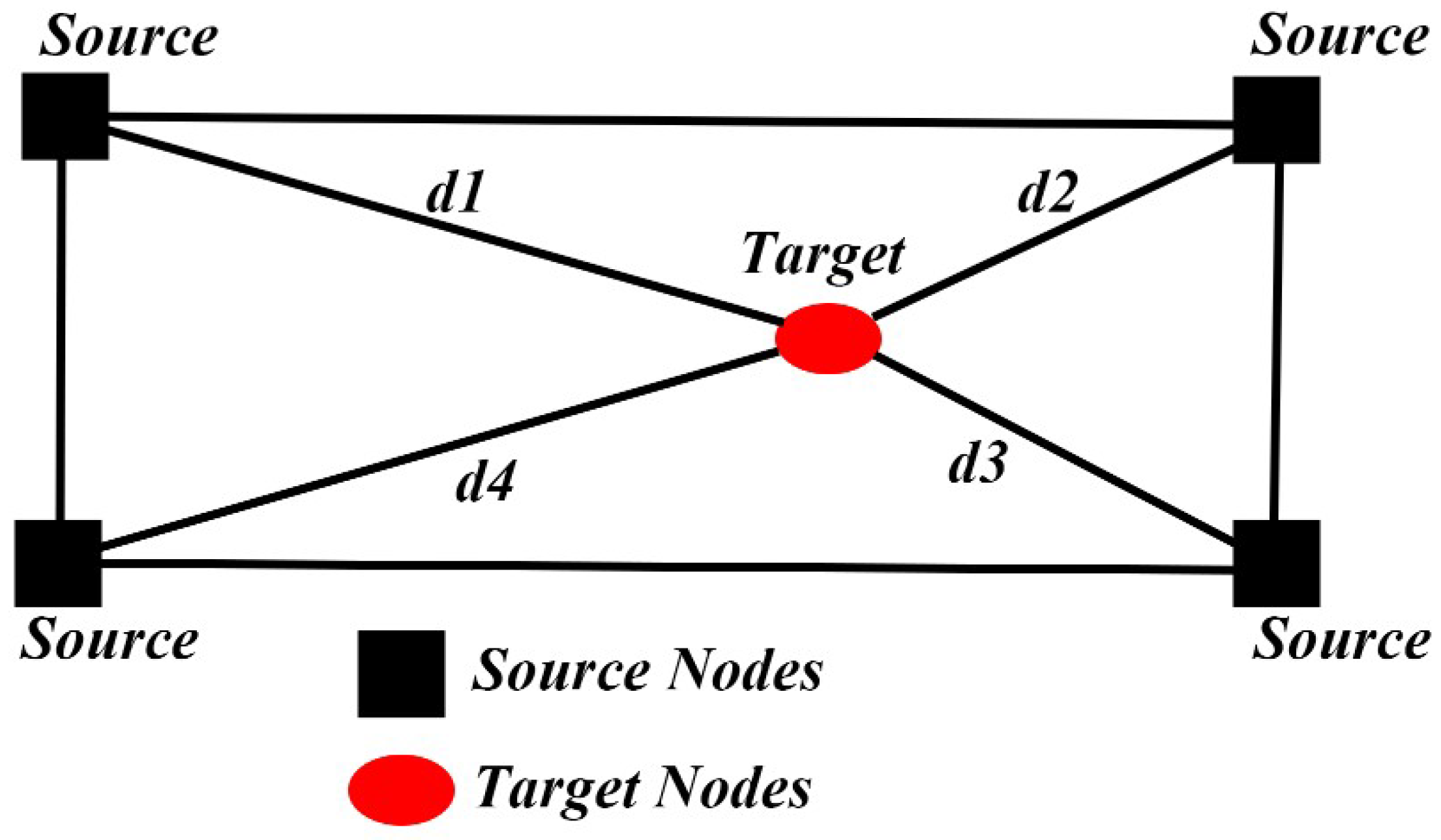
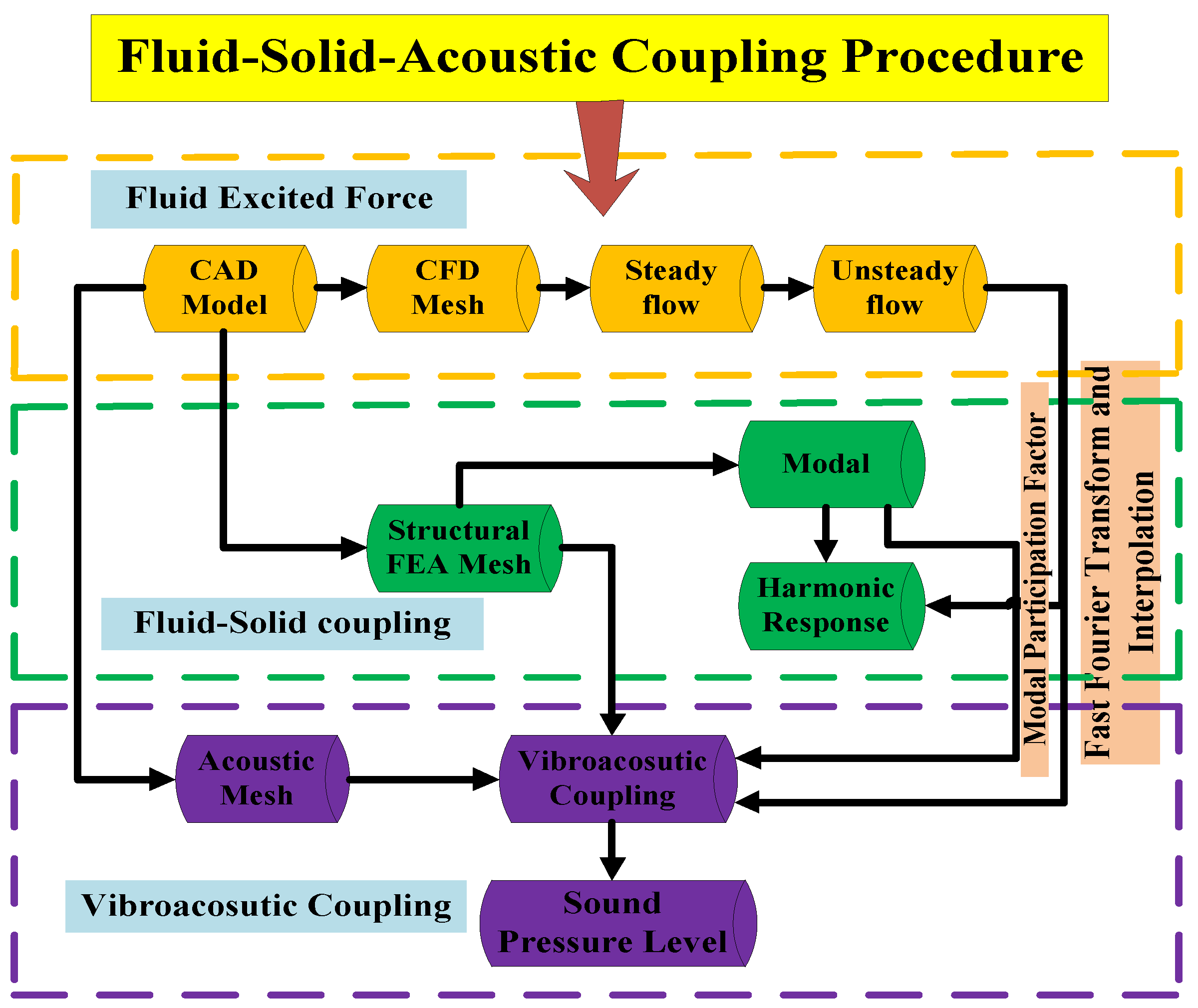
Figure 14 shows the numerical evaluation method of the volute vibroacoustic coupling. It can be seen that the one-way fluid–structure–acoustic coupling method is divided into three main steps. The first involves the acquisition of the vibrational source of the volute based on the unsteady flow calculation on the centrifugal fan, and then transformation of the extracted time-domain fluctuation data into frequency-domain data through FFT, providing basic data for the next vibration response and vibroacoustic calculation. The second steps involves the interpolation of the frequency-domain node pressure of the fluid into the corresponding structural FEM nodes according to Equation (5) (where P_i (i = 1, 2, 3, 4) is the source node pressure load, P_A is the target node pressure load, and d_i (i = 1, 2, 3, 4) is the distance from the source node to the target node; Figure 15 is a sketch of the geometric interpolation algorithm), assignment of the interpolated node pressure of the structure to the boundary loads of vibroacoustics, and then application of the structural FEM to obtain the modal participation factor of the volute. The third step involves loading the modal participation factor and vibroacoustic boundary loads that were obtained during the second step in order to calculate the volute vibrational sound radiation using the modal superposition vibroacoustic method.

$$P_{\mathrm{A}}=\frac{P_1\frac{1}{d_1}+P_2\frac{1}{d_2}+P_3\frac{1}{d_3}+P_4\frac{1}{d_4}}{\frac{1}{d_1}+\frac{1}{d_2}+\frac{1}{d_3}+\frac{1}{d_4}}$$

(22)

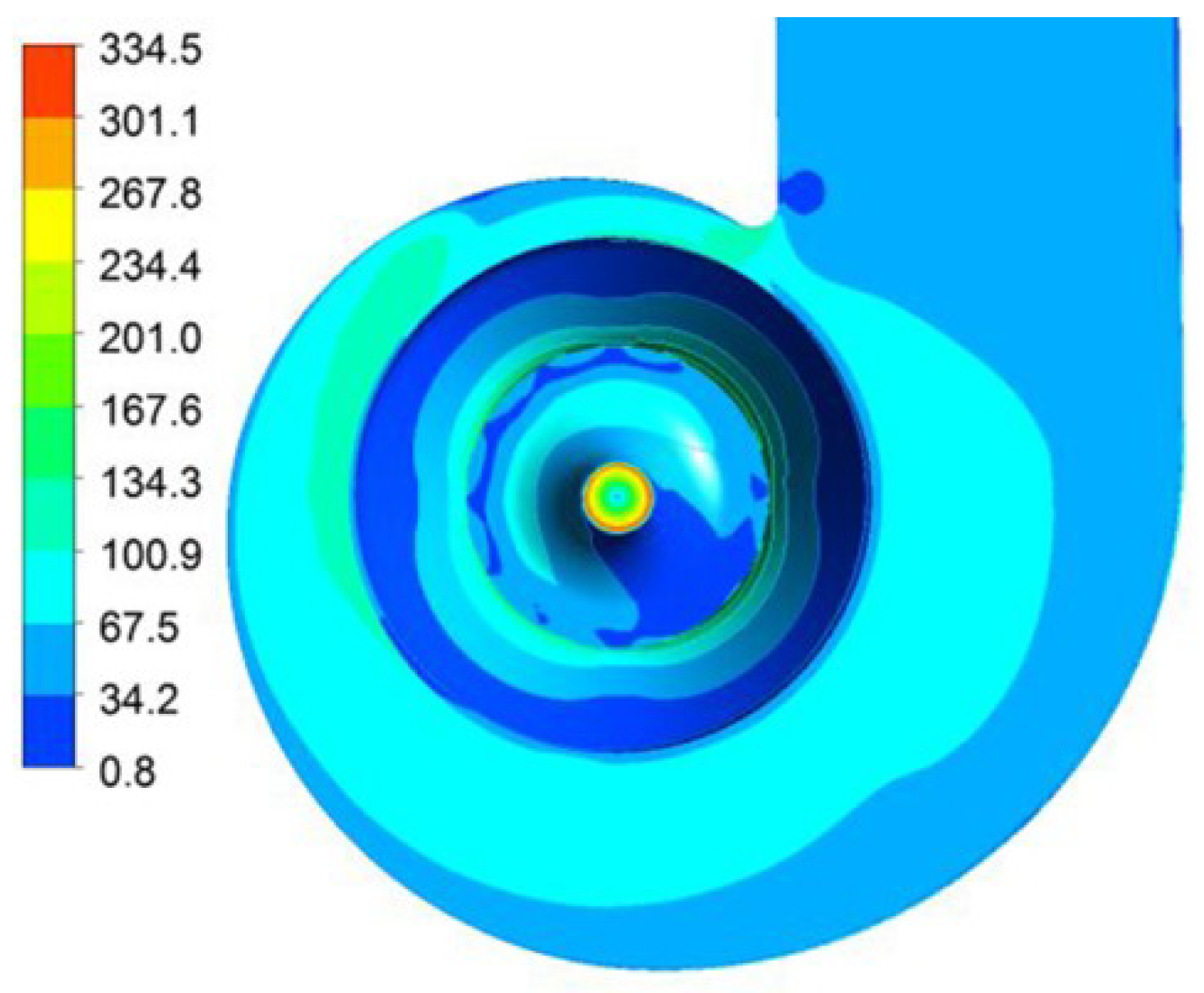
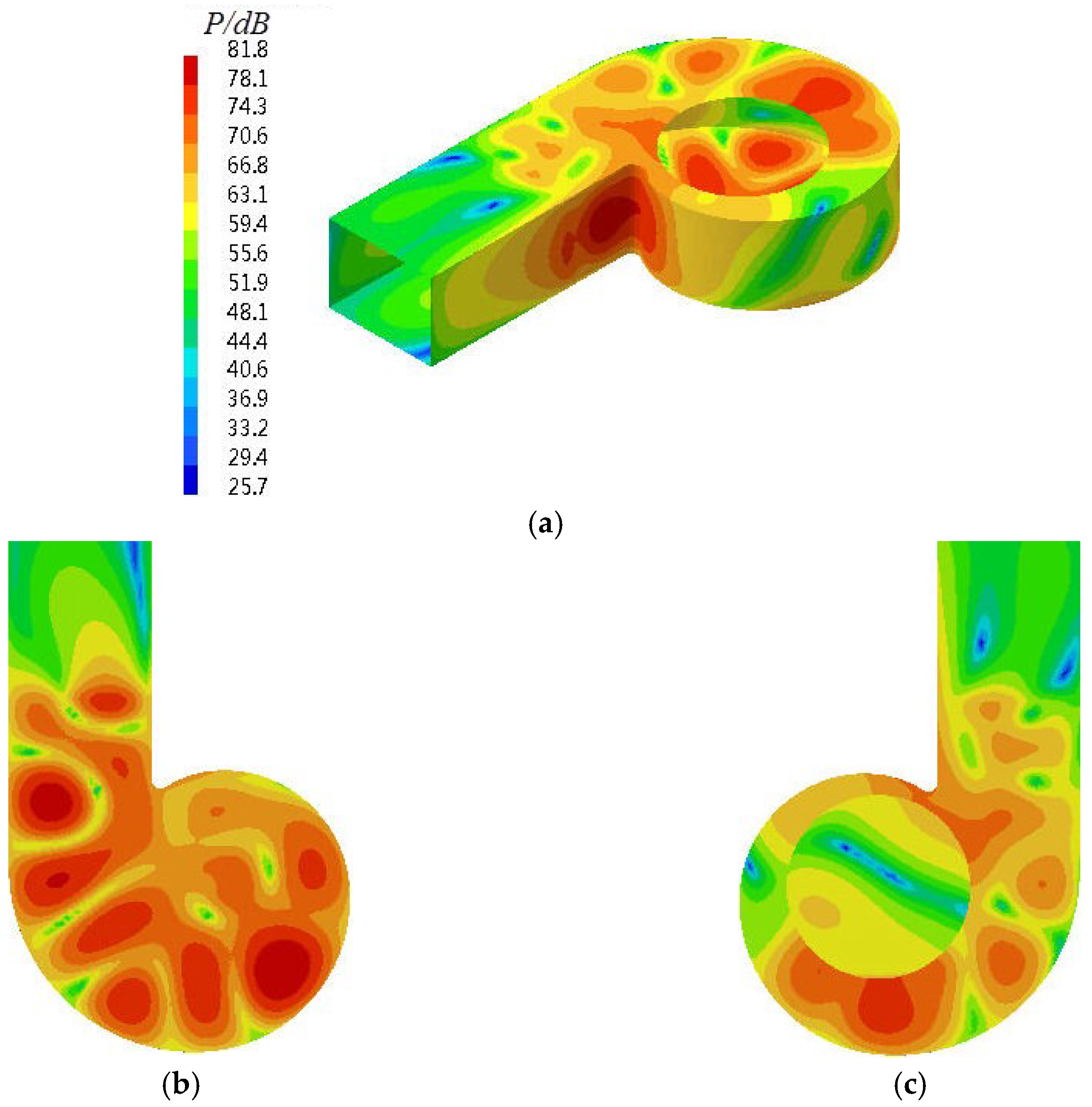
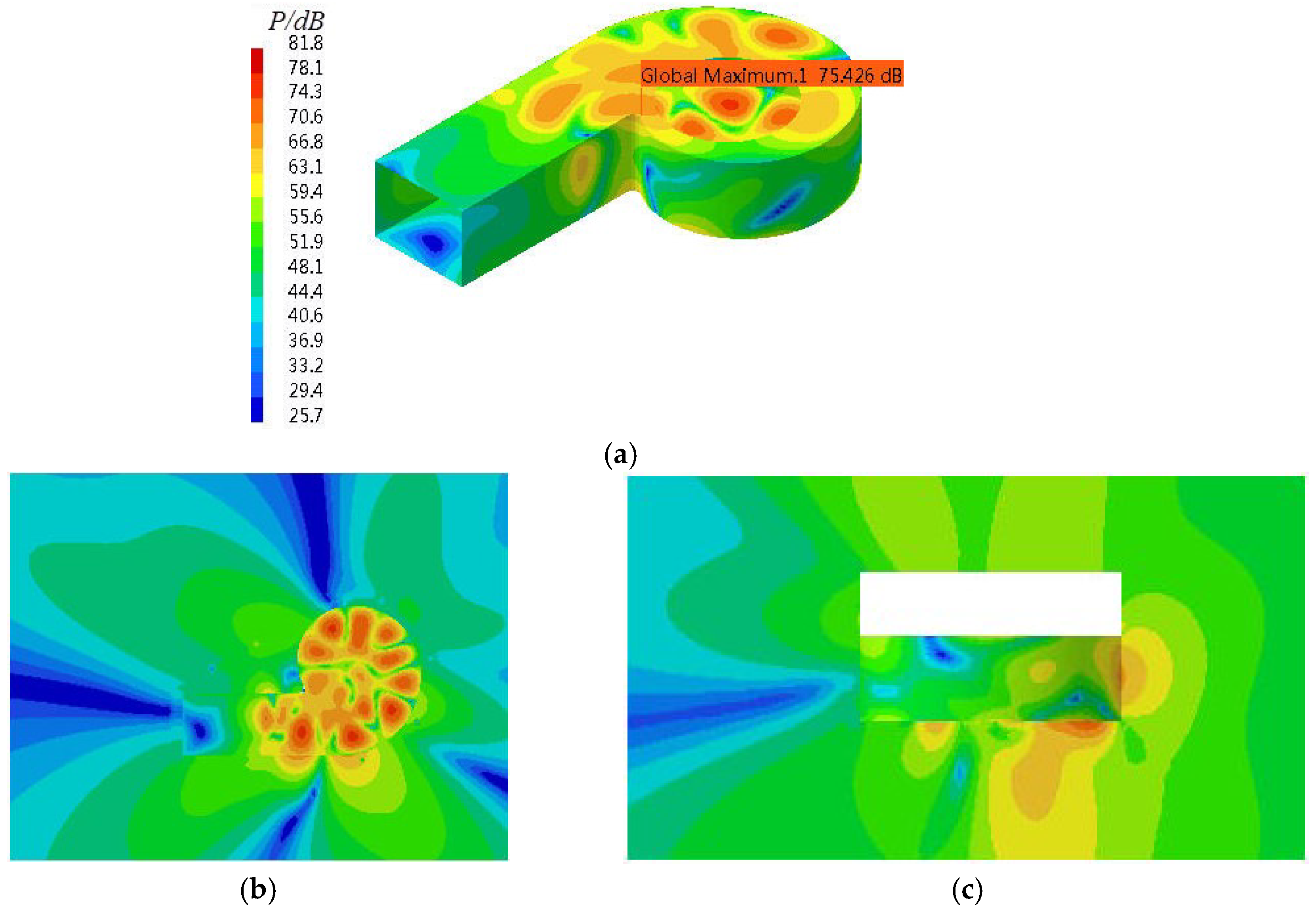
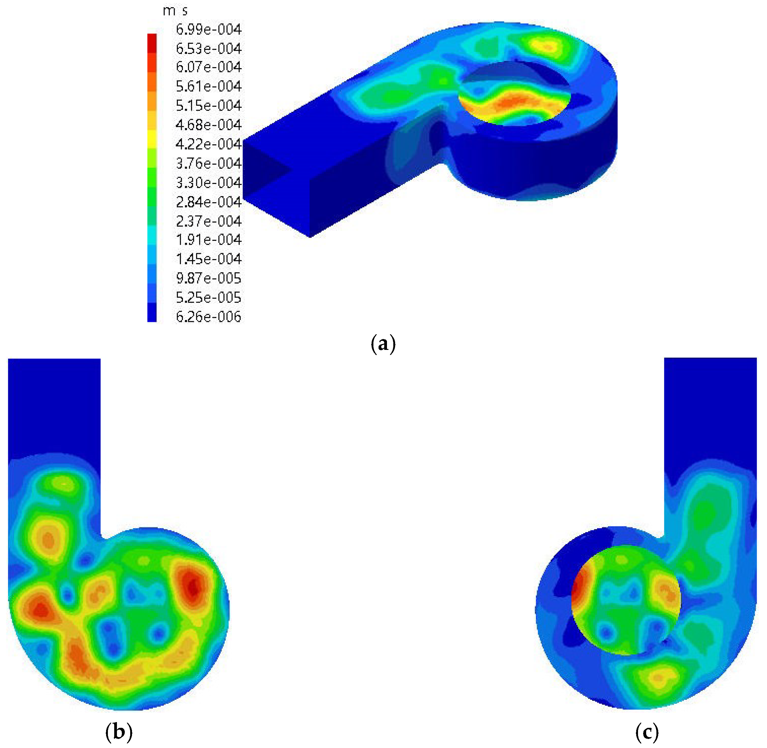
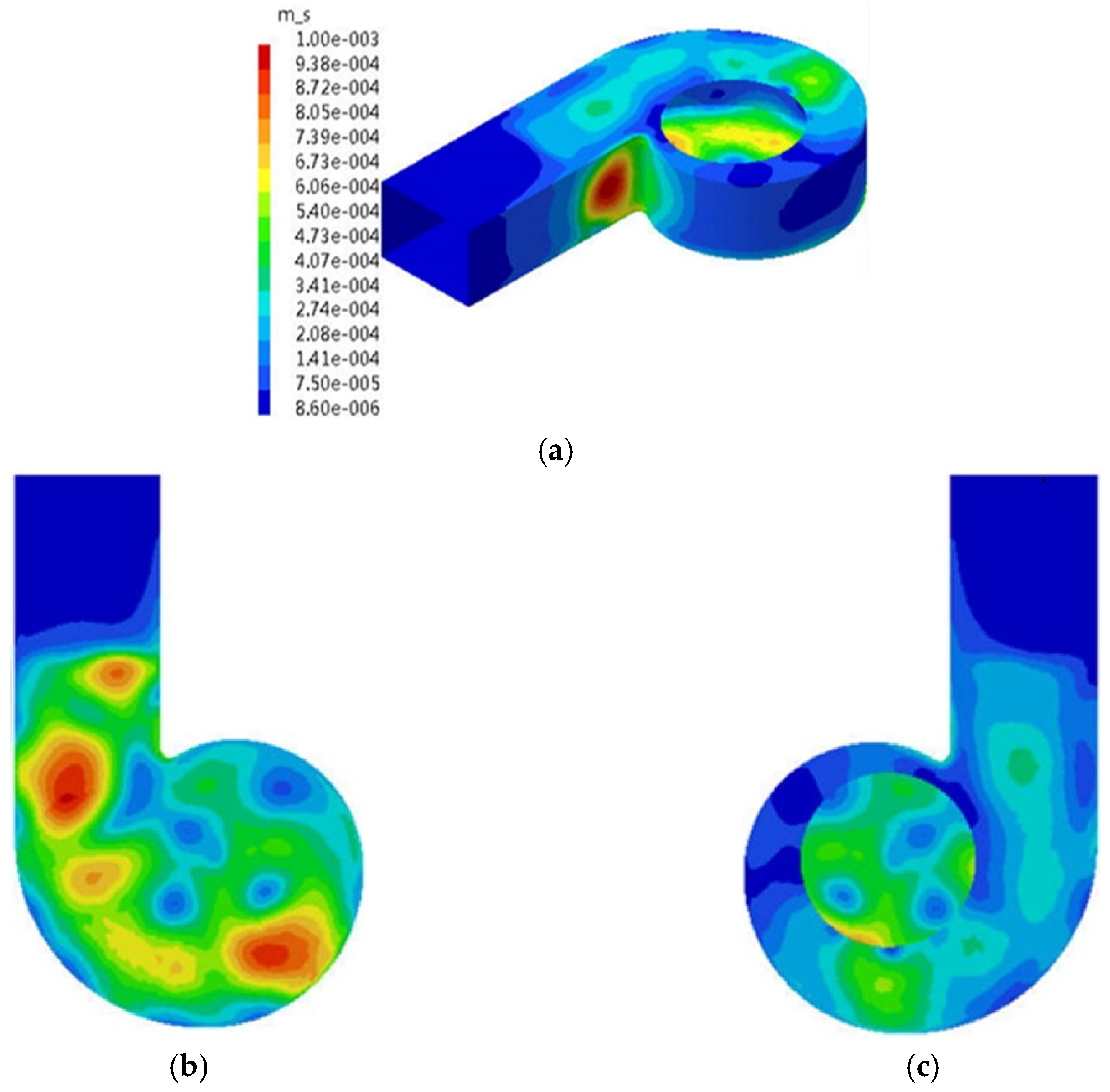
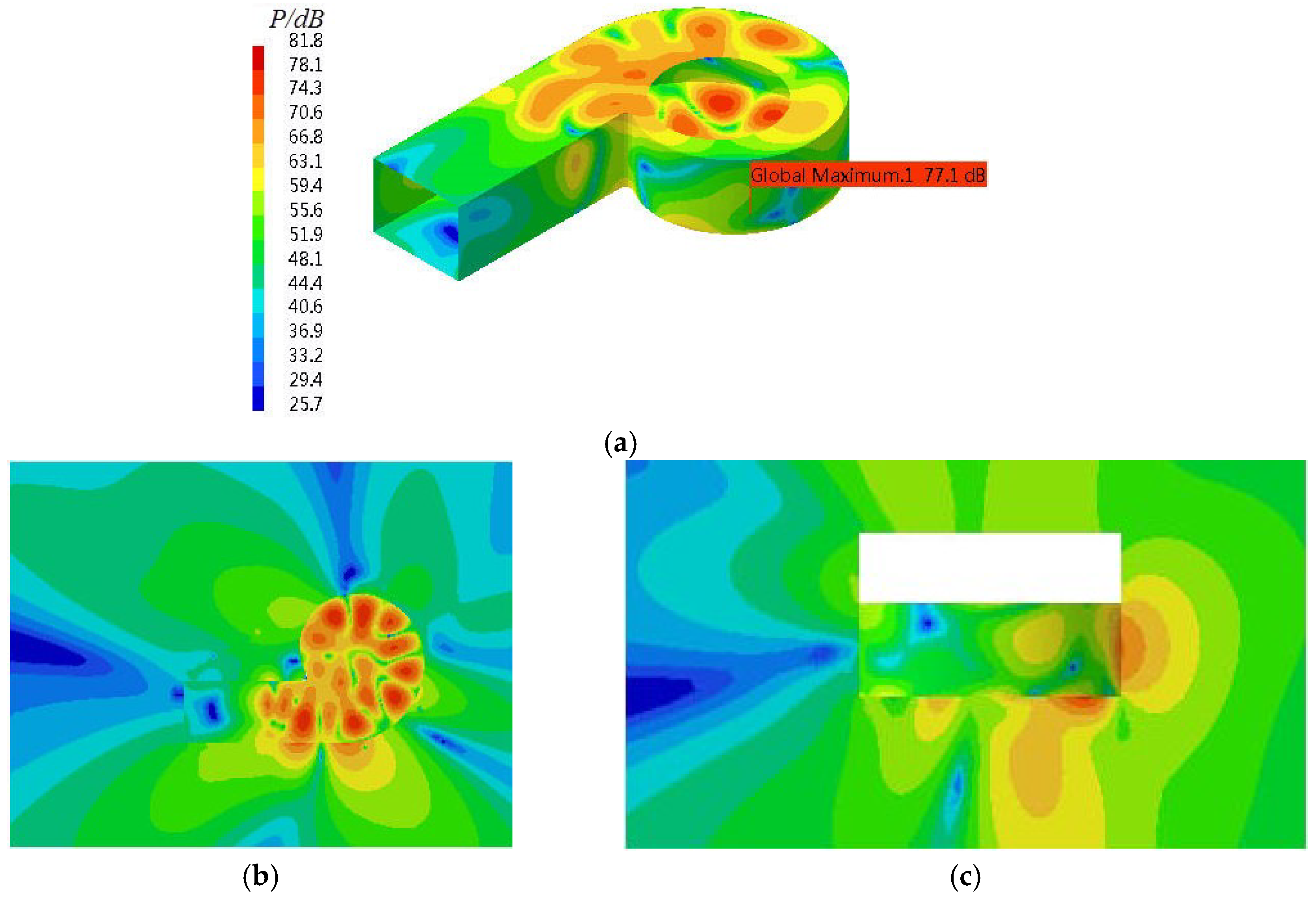
Figure 16 presents the spectrum chart of the vibrational sound radiation of volute casing, and the vibrational noise at the fundamental frequency (BPF) is obvious. Besides, the distribution of the vibrational sound radiation and the normalized velocity of the volute casing surface at the fundamental frequency is presented in Figure 17 and Figure 18. It can be observed that the distribution shape of the surface sound pressure and surface normal velocity on the volute have identical characteristics, and the outlet of the volute side panel near the volute tongue region and the volute back panel at 180° from the tongue presented very strong vibrational acoustic radiation values. In addition, the previous study [36] showed that the normal vibration velocity of the volute was the decisive factor that determined the volute surface acoustic radiation. Moreover, the theoretical derivation of Section 4.1 (according to Equation (19)) shows that the acoustical power that characterized the vibrational acoustic energy is also a quadratic function of the vibrational velocity (according to Equation (19), Zhou [22]) indirectly reducing the volute surface acoustical radiation through a decrease in the surface normal velocity of the volute casing.

5. Vibroacoustic Optimization Strategy

5.1. Optimization Objective Selection and Volute Panel Thickness Parametrization

Determining the appropriate optimization objective function is the key problem of optimizing calculations. Section 4.1 of this paper provides two means to control vibroacoustics. Control method (1) can be used to modify the geometrical shape of the volute tongue or wavy edge of the blade to weaken the pressure fluctuations on the volute casing. Control method (2) can be used to modify the model geometry, thickness distribution, and constrained position, and reduce the modal shapes. However, the shapes and natural frequency are determined by the structural thickness distribution, structural stiffness, and the constrained position. The modal shapes can be changed by controlling the thickness distribution, when the geometry, stiffness, and constrained position of the structure are fixed.

Concerning the studied centrifugal fan volute with several welding panels, this study developed an optimization method of vibroacoustics by changing different panel thicknesses (FT, BT, and ST) to attenuate the volute vibrational acoustic radiation. Regarding vibroacoustic optimization, we must first determine the optimization target function. From the literature review, it is generally considered that the uniform sound pressure at the received position or the radiated sound power at the structural surface should be set as the optimization function. The selection of the target function depends on the research problems, and the target function is divided into two categories according to different attributes. One is a noise optimization problem (internal noise control problem) applied in a closed domain. In this case, one or a few sound pressure levels of a specific measuring point are taken as the target function [24,25,26,27]. Concerning the noise control problem in the open domain, the external acoustic power on the structural surface was chosen as the optimal target function. This method has been proven by many scholars [24,25,37].

For the type of target function, the sound pressure at the arranged receiving position can be clearly determined, but it may result in judgments distortion, such that a low sound pressure value at an arranged position may be obtained, and a high sound pressure value at other points can be presented. Thus, it is very important to choose such target functions. Fortunately, Marburg [38] proposed an improved target function (F), which is defined as follows:

$$F={\tilde{F}}^{\frac{1}{n}}={(\frac{1}{{\omega }_{\max }-{\omega }_{\min }}{\displaystyle {\int }_{{\omega }_{\min }}^{{\omega }_{\max }}\varphi \left\{p_l(\omega )\right\}d\omega })}^{\frac{1}{n}}$$

(23)

In Equation (23), $\varphi \left\{p_l\left(\omega \right)\right\}$ represents the given weighting function, which is replaced by the following equation:

$$\varphi \left\{p_l(\omega )\right\}=\{\begin{array}{cc}{(p_l-p_{ref})}^n,& p_l>p_{ref}\hfill \\ 0,& p_l<p_{ref}\hfill \end{array}$$

(24)

Where n = 1, which is the average value of sound pressure in the frequency spectrum; and n = 2, which is the root mean square (RMS) value of the sound pressure.

For the second type of problem, Koopmann and Fahnline [6] proposed an optimization method that takes the external radiated sound power as the target function, and is suitable for the optimal noise control method in this study. They provided the root mean square (RMS) expression of sound pressure in an enclosed space as follows:

$$W={\displaystyle \underset{S}{\int }\mathrm{Re}(I_n)}ds=\frac{1}{2}{\displaystyle \underset{S}{\int }\mathrm{Re}(p{v}_n^{*})}ds$$

(25)

Where S refers to the structural surface, and the structural surface is discretized based on FEM. At this time, the structural radiated sound power can be regarded as the sum of the individual radiated sound power on the FEM mesh [39]. Thus, after organization, Equation (25) can be changed to the following:

$$W={\displaystyle \sum }_{\mathrm{j}=1}^{N_e}{W}_j=\frac{1}{2}Re({\displaystyle \sum }_{\mathrm{j}=1}^{N_e}\frac{1}{2}{\displaystyle \underset{S_j}{\int }{p}_j{v}_{nj}^{*}dS})$$

(26)

In the formula:

• ${\mathrm{N}}_e$—the number of finite elements on the structural casing;
• $S_j$—the area of jth finite element, ${\mathrm{m}}^2$;
• ${\mathrm{P}}_j$—the sound pressure of jth finite element, ${\mathrm{p}}_{\mathrm{a}}$;
• ${\mathrm{v}}_{nj}^{*}$—the normal velocity of jth finite element, $\mathrm{m}/\mathrm{s}$.

The vibrational noise of the volute structure of the marine centrifugal fans that is studied in this paper belongs to the typical external opening noise radiation problem. Therefore, the second type of optimization target function should be adopted.

The previous analysis in Section 4 shows that the structure modal shape can be changed by controlling the structural thickness distribution. Therefore, the volute thicknesses of the three panels (FT, BT, and ST in mm) were specified as the design variables. Thus, the design objectives can be achieved by adjusting the combination of different volute panel thicknesses in the optimization design. The thickness of each volute panel is parameterized using FEM. Figure 19 shows the volute parameterization structural FEM. Since the panel thickness of each volute is generally less than 10 mm, we assigned the panel thickness of each volute to be from four mm to 10 mm.

5.2. RBF Approximation Surrogate Models and Validation

The high computational cost of each vibration and acoustic simulation to predict the vibroacoustics performance of each volute panel thickness design makes a direct optimization approach to find an optimum low-vibration noise volute unfeasible. Indeed, an optimized cycling takes 24–26 h. In addition, the optimization process terminates due to the failure of a single simulation program. Therefore, the long time of the optimal iterative procedure is the major bottleneck in the optimization of acoustics performance for all complex structures. Instead, the use of a surrogate model, which was constructed from and used in lieu of the actual simulation model, represents a valuable alternative to increase the speed of the optimization. For this reason, a metamodeling approach was chosen for vibroacoustic optimizations. Therefore, the combination of a design of experiment (DoE) and an approximation model (AM) was used to determine the relationship between the structural design variables and the target function, and provide the basic data and models for the subsequent optimization. According to the studied centrifugal fan volute, taking each volute thickness (FT, BT, and ST) as design variables, each design variable was given five levels.

Table 3. The levels of distribution of each volute panel thickness. FT: the front panel thickness, ST: the side panel thickness, BT: the back panel thickness.

Variables	Range/mm	Levels of Distribution/mm
FT	5.00~10.0	5.00	6.25	7.50	8.75	10.0
ST	5.00~10.0	5.00	6.25	7.50	8.75	10.0
BT	5.00~10.0	5.00	6.25	7.50	8.75	10.0

provides the levels of distribution of the design variables. Due to the smaller number of design variables, the full-factor method was adopted to collect sample points of the design space constructed by the three variables collected; thus, a total of 125 sample points was collected.

For each sample point, the aforementioned vibroacoustic coupling assessment method was used to calculate the radiated sound power and the total volute mass of the volute structure surface of each combination. The approximate model approach is generally divided into two broad categories: first, least squares fitting, also known as response surface methodology (RSM); and the second, interpolation. RSM uses polynomial functions to fit the design space. In addition, the RSM fitted the complex response relationships through regression models due to the simple algebraic expression. In addition, because of the advantages of being systematic and practical, the RSM had been used in a broad range [40,41,42,43], but the approaching effect is not as good as that of neural network and other methods for highly complex functional relationships (a complex relation of nonlinear function). The radial basis function (RBF) belongs to the interpolation algorithms, and is the second approximate model method. Since the neural network model has a strong ability to approximate complex nonlinear functions, the learning speed is fast, has excellent generalization ability, and is highly fault-tolerant. It is used by many scholars and engineers in aircraft wingtips [44], highway traffics [45], turbomachinery [46], engineering optimization [47], compressors [48], gas cyclone separator [49], MMES controllers [50], and many other applications. The relationships between the vibrational sound radiation of the volute casing surface and the volute panel thickness are typically nonlinear. Thus, this study used the RBF model to approximate and fit the design space.

Figure 20 shows the fitting procedure of the vibroacoustic optimization of volute casing. It can be seen from Figure 20 that this procedure is mainly divided into two parts. The first is the creation of a design space for the collected sample points using the assessment method of vibroacoustic coupling. The FEM model of fan volute was established by UG; then, ANSA constructed FEM mesh, and the Nastran code solved the volute modal participation factor. At last, the vibrational sound radiation of volute was used by LMS Virtual Acoustics. In addition, all the calculation codes were integrated into the multi-disciplinary optimization platform, Isight. The second built an RBF approximation model (RBF surrogate model) instead of a simulation loop, as mentioned for the first part. Thus, the RBF method with Isight code was used to establish an approximate alternative model.

In fact, the approximate model can be considered an approximate approach for the physical model, in which the precision of the approximate model is affected by the number of sampling points. At present, statistical theory with analysis of variance is usually used to verify the effectiveness of an approximate model. However, the approximate model is usually tested by the complex correlation coefficient R² (0 < R² < 1) in engineering, and Shi [51] provided its mathematical expression. The closer the value of R² is to one, the more precise the approximation model. Figure 21 shows the error schematic diagram of each response surface model. In Figure 21, the Kirchhoff SPW (dB) represents the radiated sound power of the volute surface, and the mass (kg) represents the total mass of the volute. It can be seen that all the response surface models are infinitely close to the value one; thus, the approximate model that was established using the mentioned method can completely replace the real simulation loop. The parametric analysis related to the radiated sound power of the volute surface is performed, which will be discussed in the following sections.

5.3. Single-Objective Optimization Procedure

The single-objective optimization was conducted to improve the radiated sound power of the fan volute by using a weighted-average surrogate model with three design variables related to the geometries of the three-part volute panel thickness. The collection of sample points that was described in the previous text, and based on the RBF approximation model, provides the basic database and the analysis model of the target function for the optimization of the vibroacoustic coupling of the volute structure. In this part, the single-objective optimization took three panel thicknesses (FT, BT, and ST in mm) as design variables, and took the vibrational sound radiated power of the volute surface (Kirchhoff SPW (dB)) as the target function. In addition to these, the single-objective optimization was divided into two parts: the first part maintained the volute total mass as invariable, and for the second part, there was no mass constraint on the volute. Since the thickness of the volute panel is generally less than 10 mm, the author assigned the volute panel thickness as from four mm to 10 mm. Therefore, the mathematical model optimized in this section is as follows:

The objective function, W_s (minimum):

$$W_s={\displaystyle \sum }_{\mathrm{j}=1}^{N_e}{W}_j=\frac{1}{2}Re({\displaystyle \sum }_{\mathrm{j}=1}^{N_e}\frac{1}{2}{\displaystyle \underset{S_j}{\int }{p}_j{v}_{nj}^{*}dS}),(\mathrm{vibrational}\mathrm{sound}\mathrm{radiated}\mathrm{power}\mathrm{of}\mathrm{volute}\mathrm{surface},\mathrm{W})$$

(27)

Variables:

[FT, ST, BT]

(28)

Constrained conditions:

$$\begin{array}{l}4\le \mathrm{FT}\le 10\\ 4\le \mathrm{ST}\le 10\\ 4\le \mathrm{BT}\le 10\end{array}$$

(29)

Constrained variable:

$$M_T=S_{FT}\cdot FT+S_{ST}\cdot ST+S_{BT}\cdot BT,(\mathrm{total}\mathrm{mass},\mathrm{kg})$$

(30)

Defining the sound power level as follows:

$$10\times {\lg }^{(W_s/W_{ref})}$$

(31)

In Equation (31), $W_{ref}$ represents the reference value of sound power, $W_{ref}=1\times {10}^{-12}$ $\mathrm{W}$

Figure 22 shows the flow chart of the single-objective optimization. The single objective optimization uses the simulated annealing algorithm (ASA) to implement a global search. The optimal result of the approximate model in the previous text is assigned as the initial value, and the global optimization iterates 10,000 steps and takes 12 minutes. Then, the value is locally optimized using mixed integer sequential quadratic programming (MISQP), which iterates more than 12 steps in several seconds. The results of the single-objective optimization of the vibroacoustics of a volute surface will be discussed in the following sections.

5.4. Multi-Objective Optimization Procedure

In fact, the parameters of the vibrational sound power and total mass on the volute surface are somewhat contradictory. Thus, a multi-objective optimization method is needed to obtain the optimal volute thickness combination. The definition of the multi-objective optimization mathematical model is presented as follows:

The objective function, W_s, M_T (minimize):

$$W_s={\displaystyle \sum }_{\mathrm{j}=1}^{N_e}{W}_j=\frac{1}{2}Re({\displaystyle \sum }_{\mathrm{j}=1}^{N_e}\frac{1}{2}{\displaystyle \underset{S_j}{\int }{p}_j{v}_{nj}^{*}dS}),\mathrm{vibrational}\mathrm{sound}\mathrm{radiated}\mathrm{power}\mathrm{of}\mathrm{volute}\mathrm{surface},\mathrm{W}:$$

(32)

$$M_T=S_{F\mathrm{T}}\cdot FT+S_{ST}\cdot ST+S_{BT}\cdot BT,(\mathrm{total}\mathrm{mass},\mathrm{kg})$$

(33)

Variables:

[FT, ST, BT]

(34)

Constrained conditions:

$$\begin{array}{l}4\le \mathrm{FT}\le 10\\ 4\le \mathrm{ST}\le 10\\ 4\le \mathrm{BT}\le 10\end{array}$$

(35)

Figure 23 presents a flow chart of multi-objective optimization. The multi-objective genetic algorithm termed NSGA_2 was adopted to solve the multi-objective optimization with the optimal value obtained by taking the single-objective optimization of specific mass constraints as the initial values. The global search iterates 4800 steps, and the Pareto frontier solutions are marked. A solution satisfying the requirement is selected as the initial value of MISQP for mixed integer quadratic programming; then, the final solution satisfying the engineering requirement is obtained by iterating 15 steps again. Finally, the vibroacoustic estimation method mentioned in Section 4.3 is used to verify the precision of the optimal solution. The multi-objective optimization results will be discussed in the following sections.

6. Results and Discussion

6.1. Results of Sensitivity and Parametric Analysis

In order to investigate the influence of each design variable on the optimization objectives, it is necessary to perform the sensitivity analysis for the design variables. Sensitivity analysis is performed by studying the correlations between the design variables and the objectives. Figure 24 shows the correlation distribution of design variables and optimization objectives (Kirchhoff SPW, volute mass on the volute structure surface); the correlation theory and definition referred to the reference [52]. The positive value indicates that the optimization objective is proportional to the design variable, and otherwise is an inverse relationship. The closer the absolute value of the coefficient is to one, the higher the degree of correlation. It can be seen from Figure 24 that ST had the largest influence on all the objectives, followed by FT, then BT. Concerning radiated sound power, ST and FT present an inverse proportionality to the radiated sound power, which means that the larger the volute panel thickness (ST and FT), the smaller the radiated sound power.

However, the relationship diagram between each volute panel (ST, BT, FT) and objective functions (the Kirchhoff SPW or the total mass of the volute) in Figure 25 shows that BT and FT present nonlinearity characteristics for the acoustic power of the volute surface. With an increase of BT value, the vibrational radiated sound power of the volute surface increases first, and then decreases, and FT value presents the opposite change. However, the volute radiated sound power decreases with ST value if the ST does not exceed nine mm. This means that each panel thickness (BT, ST, FT) has an optimal value that satisfies the radiated sound power minimum. However, Figure 25 only shows the influence of each single thickness variable on the radiated sound power (the other two variables remain unchanged; the relationship between the other two variables and the noise radiation is determined). To determine the relationship between each variable combination (BT–ST; FT–ST; FT–BT) and the acoustic radiation power, Figure 26 gives the influence of each two-panel thickness variation on the radiated sound power. It can be observed that the FT–ST and BT–ST combinations present similar distribution characteristics. Therefore, the Kirchhoff SPW basically remained a constant smaller value when the ST was greater than 7.0 mm, and the BT was less than 8.5 mm or the FT was less than 7.0 mm. In addition, as the FT is larger and the BT is smaller or the FT and BT are both smaller (less than 5.5), the Kirchhoff SPW is observed to have a smaller value as shown in Figure 26c. Besides, linear relationships could be seen in Figure 25b, which means that the thicker the thickness of each volute panel, the greater the total mass of the casing.

In conclusion, the variation in ST is the most sensitive to the sound radiation power of the volute structure surface, while FT is the second-most sensitive, and BT is the least. Therefore, it is possible to obtain the smallest value of radiated sound power of the volute surface by optimizing the panel thickness combination (increasing the ST value and decreasing the FT and BT values).

6.2. Results of Optimization.

After optimization, the vibrational radiated sound power of the volute surface is greatly reduced.

Table 4. Massless constrained optimization results.

Table Title	FT (mm)	ST (mm)	BT (mm)	Ws/(dB)	MT (kg)
Original	6.000	5.000	6.000	63.78	86.592
Optimized	4.000	10.00	4.000	54.38	102.29
Numerically validated	4.000	10.00	4.000	56.25	102.29

shows the massless constrained optimization results (the “optimized” represents the calculation results of the approximate model, and the “numerical validated” represents the vibroacoustic analysis with the optimum values). It can be seen that the radiated sound power on the volute structure surface decreases by 9.4 dB when ST increases to a maximum, while BT and ST locate at minimum values; unfortunately, at the same time, the volute total mass increases by 18.13%.

Table 5. The optimization results with the volute total mass invariable.

Table Title	FT (mm)	ST (mm)	BT (mm)	Ws / (dB)	MT (kg)
Original	6.000	5.000	6.000	63.78	86.592
Optimized	4.335	7.470	4.000	57.52	86.592
Numerically validated	4.335	7.470	4.000	58.68	86.592

shows the optimization results with the volute total mass invariable. Even though the volute total mass remains the same, the radiated sound power on the surface of the volute will also be weakened by an average of 6.3 dB. In addition, the radiated sound power spectrum of the volute structural surface shown in Figure 27 also shows that the single-objective optimization significantly improves the radiated sound power on the volute surface at the fundamental frequency (BPF).

In order to better understand the improvement effect of optimum panel thickness combinations on vibroacoustic performance before and after optimization, the comparison of distribution of vibrational sound radiation before and after the total mass invariable optimization at the fundamental frequency are given in Figure 28 and Figure 29. From the comparison, it can be concluded that the sound pressure of the vibrational radiation close to the tongue on the side volute is greatly reduced by optimization, and the other sound pressure of the vibrational radiation on the other area is also weakened to varying degrees. In addition to these results, the optimization also changed the directivity distribution of acoustical radiation, and very strong directivity was produced on the back panel side of the volute.

The multi-objective optimization results, which took the volute surface vibrational radiated sound power and the total mass of the volute as the objective function of the optimization model, conformed to the actual needs. Multi-objective optimization solutions are not unique, and are usually presented in the form of solutions (Pareto front solutions). According to the distribution of Pareto front solutions in Figure 30, it can be seen that the radiated sound power on the volute surface and the total mass of the volute show an approximately linear inverse proportional relationship, and a smaller vibrational sound power can be obtained, when the volute mass (mass increase control: ± three kg) changes within a small range. Moreover, if the volute mass increased by two kg, the total acoustic power of the volute surface and the radiated sound power at BPF decreased by 7.3 dB and 6.9 dB, respectively, as shown in

Table 6. The multi-objective optimization results.

Title	FT (mm)	ST (mm)	BT (mm)	Ws/(dB)	MT (kg)
Original	6.000	5.000	6.000	63.78	86.592
Optimized	4.001	7.935	4.010	56.53	88.549
Numerically validated	4.001	7.935	4.010	57.16	88.549

and Figure 31. In addition to these, Figure 32 shows a comparison of the radiated sound power of the volute structure surface after multi-objective optimization. It can be seen that after optimization, the multi-objective optimization presents the same noise reduction effect on the volute structure surface as the single-objective optimization. In addition to these, the radiation sound pressure close to the tongue on the volute front panel is greatly reduced, the sound pressure is lower (under 10 dB) than at the other parts of the volute, and the sound pressure of the other volute parts is also greatly weakened. In summary, the radiated sound power of the volute structure surface obtained using the multi-objective optimization method is further reduced by nearly one dB compared to that of the single-objective optimization with mass constraints. It can be concluded that the optimization effect of the multi-objective method is obviously better than the single-objective optimization for this studied fan. Even considering the two conflicting objective functions, the multi-objective optimization can achieve a more balanced effect.

Generally, the noise-reduction mechanism of single and multi-objective optimization is attributed to the major factor: the normal vibration velocity of the three-part volute surface, which was changed to be smaller by controlling the thickness combination with the unsteady aerodynamics determined and volute geometry fixed. The previous study [36] showed that the normal vibration velocity of the volute surface was the decisive factor that determined the radiated sound power. To comment on this major noise-reduction mechanism, the comparison of the normal vibration velocity of the volute surface before and after optimization were presented in Figure 18 and Figure 33. It indicates that the normal vibration velocity of the volute surface was greatly diminished (especially the tongue region) after optimization, which inevitably leads to a significant reduction for the radiated sound power of the volute surface, as shown in Figure 32. In addition, the parametric analysis indicates that ST had the largest influence on sound radiated power of volute surface, followed by FT, and then BT. The sound radiated power of the volute surface could be sharply reduced if ST was much larger (larger than seven mm for this fan), while BT and FT were designed as lower values (the BT was less than 8.5 mm, and the FT was less than 7.0 mm for this fan). Less noise radiation could be achieved if the ST increased over a certain limit (the setting extremum), but this can lead to unpredictable mass gain and increased costs.

7. Conclusions

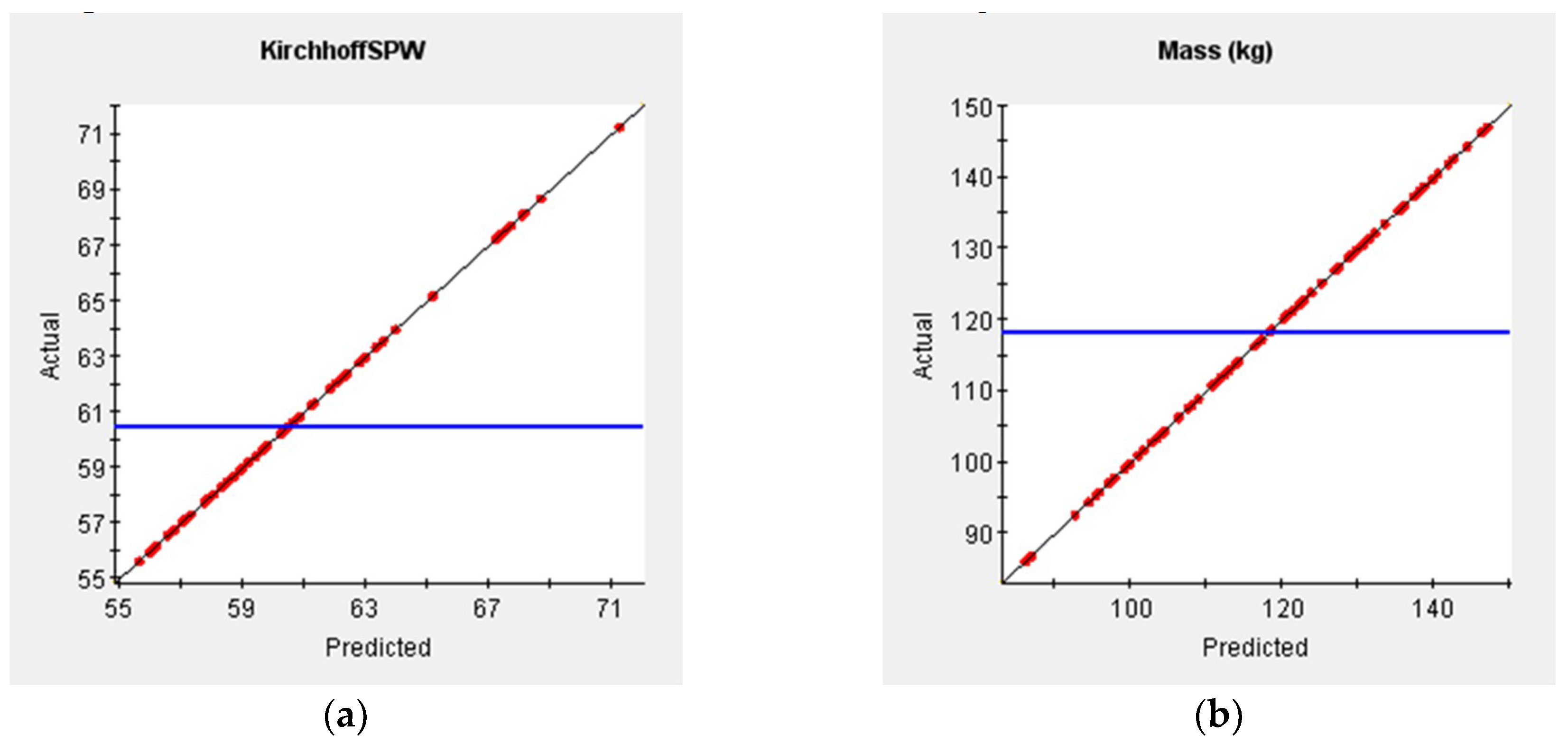
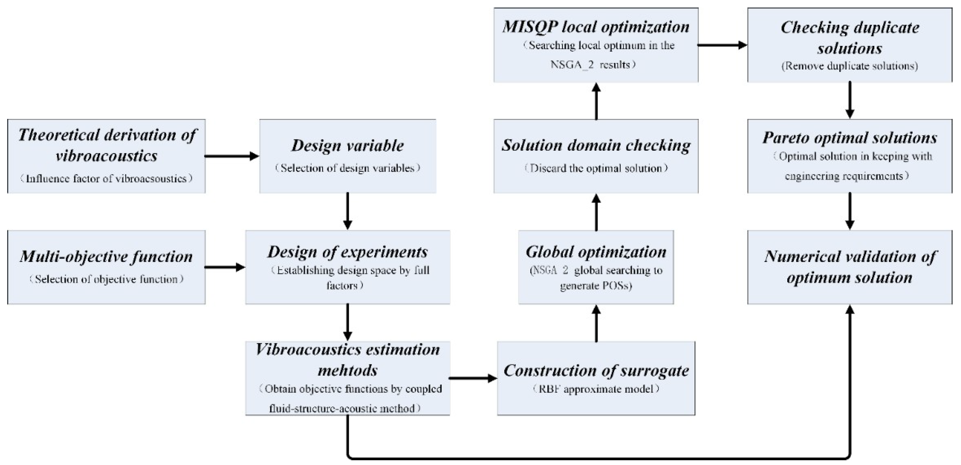
To reduce this type of vibrational sound radiation, a vibrational noise control method of multi-disciplinary optimization that considered the influence of vibroacoustic coupling was proposed. The strategies employed in the vibroacoustic optimizations based on DoE and RBF optimization techniques were proved to be highly successful, and various optimal solutions were analyzed. Some preliminary conclusions are obtained in this paper as follows:

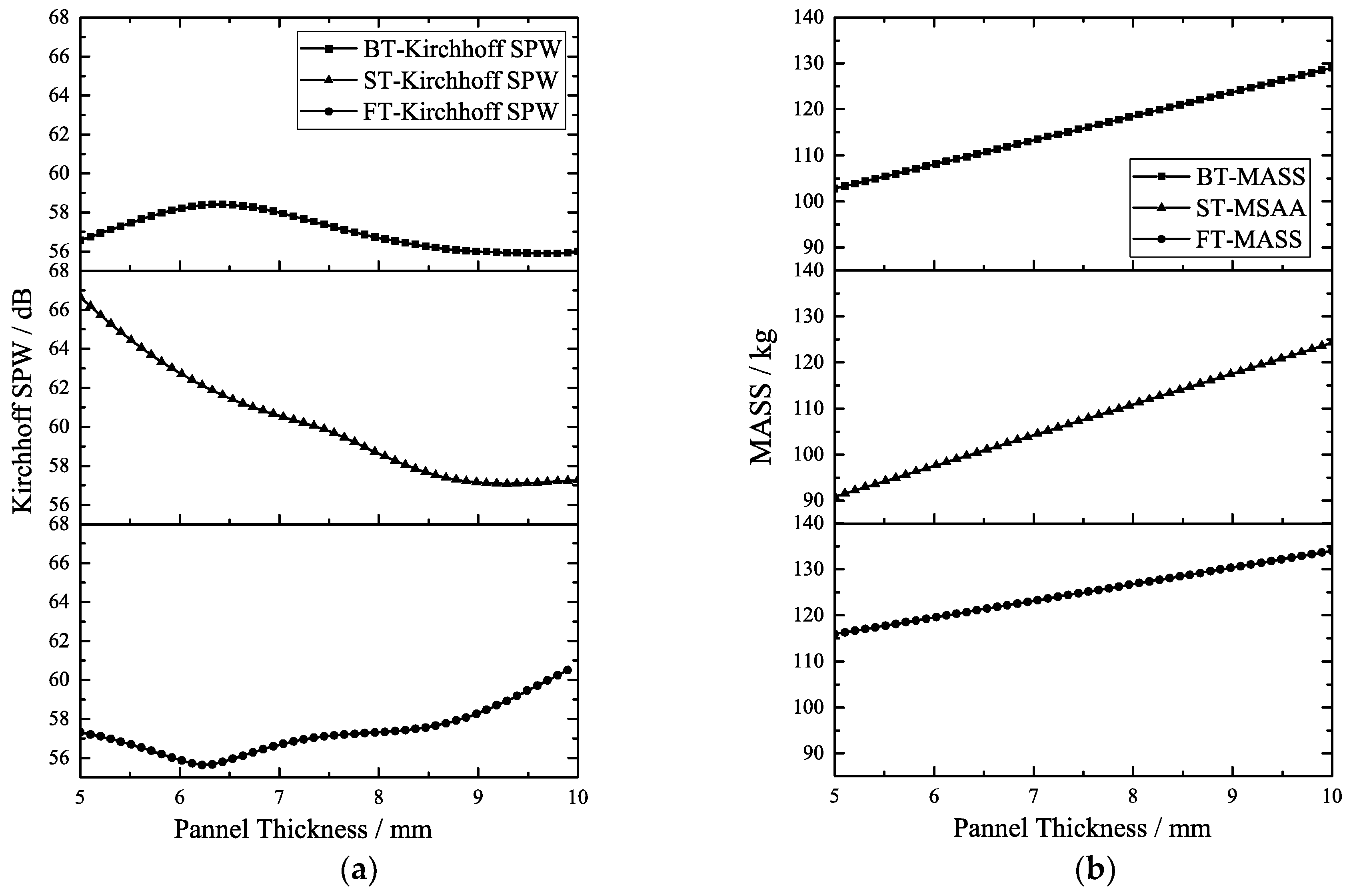
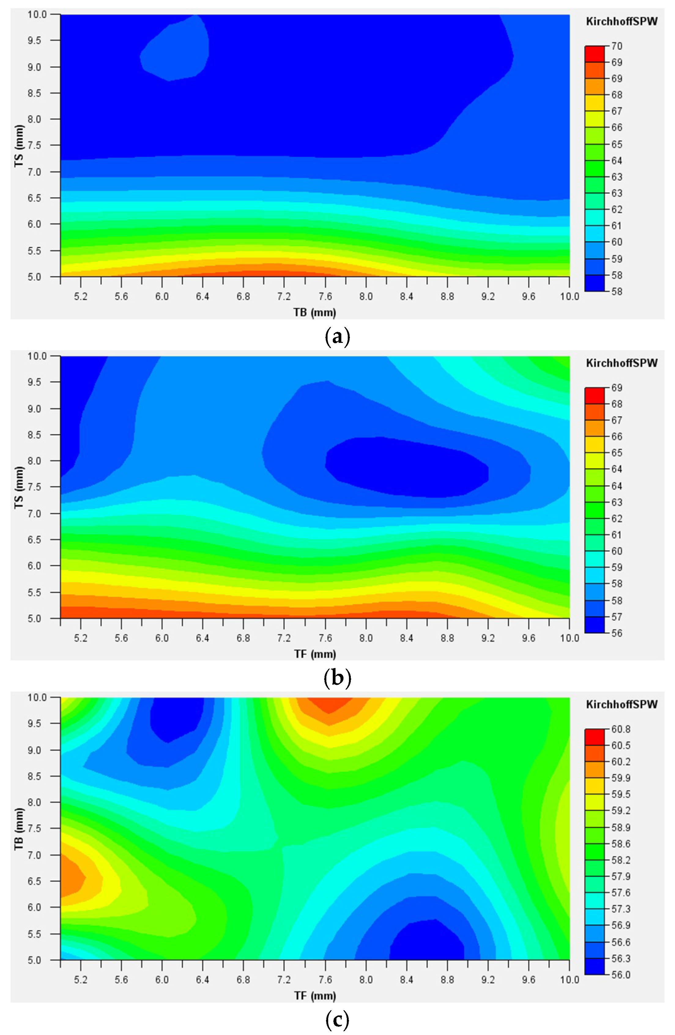
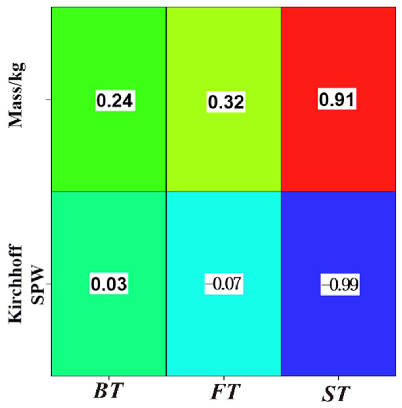
(1) The optimization results indicate that the three-part volute structure has an optimal thickness combination maintaining the volute mass constant, and the optimal design of the volute radiated sound power can be greatly reduced without any increase in material cost. Besides, the sensitivity analysis showed that ST is the most sensitive to the volute radiated sound power, followed by BT, and then FT, which is the smallest.

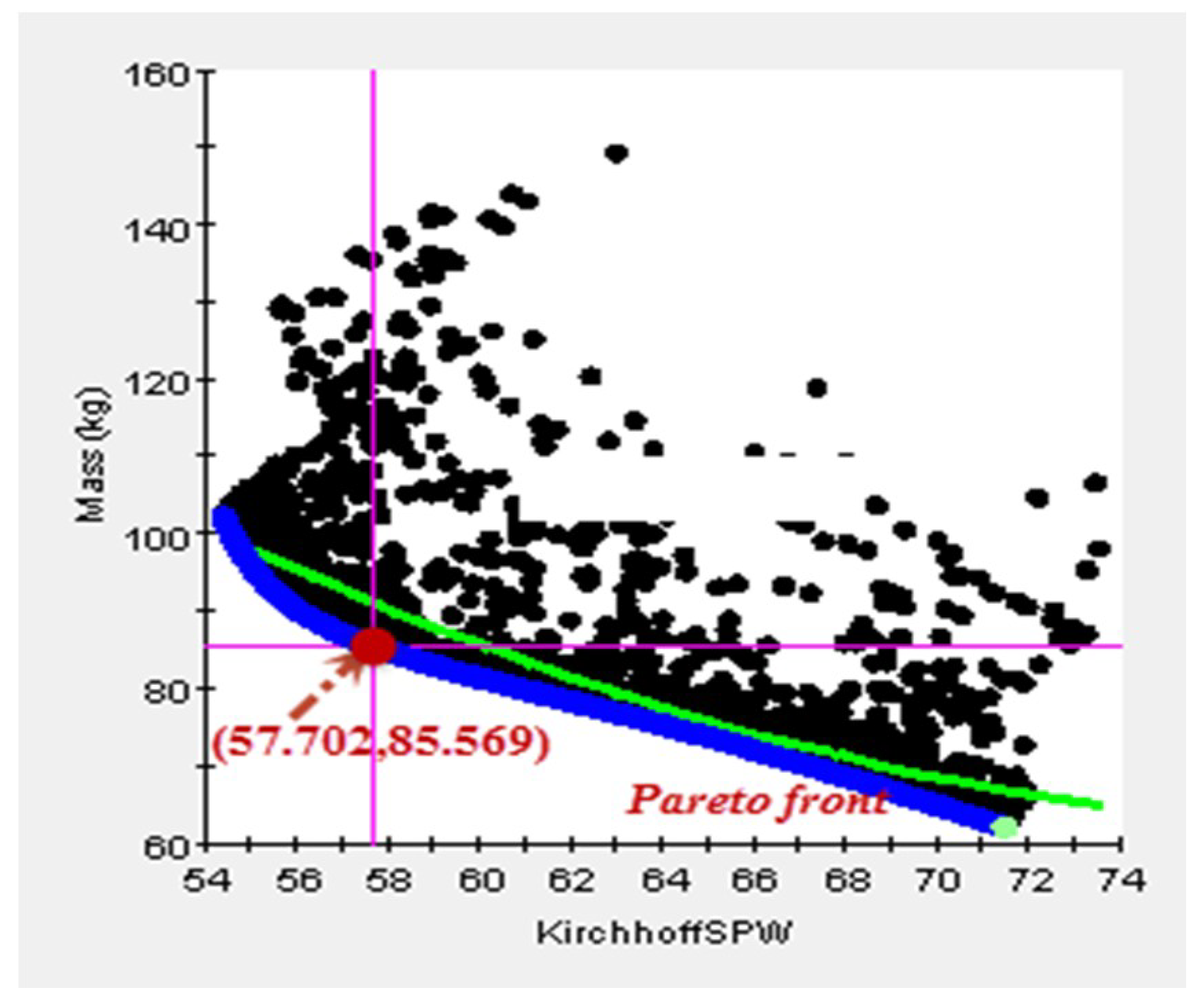
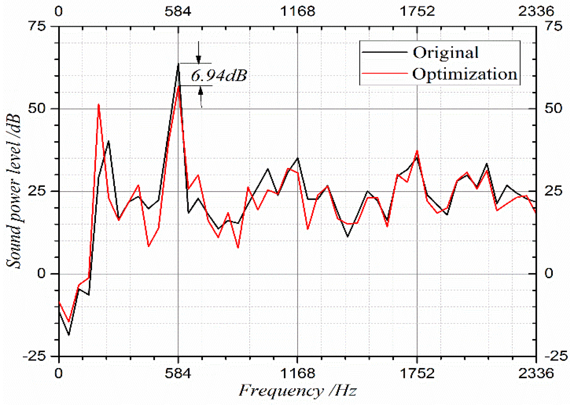
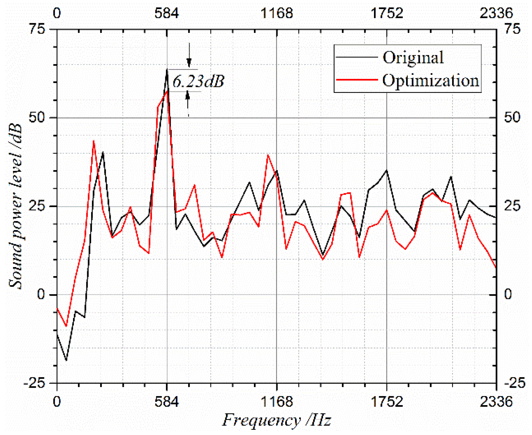
(2) The optimization process achieves the purpose of reducing the radiated sound power of the centrifugal fan volute. The radiated sound power on the volute casing surface decreased by 6.3 dB with mass constraint. Without a strict constraint of the volute mass, the optimization can be further applied to get a better thickness combination of the volute, thereby achieving better optimized vibrational noise results. The multi-objective optimization was more advantageous. It was found that the volute acoustical radiated power on the volute surface decreased by 7.3 dB when the total mass of the volute slightly increased (±3 kg). The optimization in this study provides an important technical reference for the design of low vibroacoustic volute centrifugal compressors and fans whose fluids should be strictly kept within the system without any leakage.

(3) In addition, the optimized thickness combination effectively reduces the normal vibration velocity of the volute surface, especially the volute tongue region, and thus significantly reduces the volute vibration radiation, which is also the noise reduction mechanism of this optimization method.

References

1. Koopmann, G.H.; Cunefare, K.A.; Neise, W. Fan casing noise radiation. J. Vib. Acoust. 1991, 113, 37–42. [Google Scholar] [CrossRef]
2. Citarella, R.; Federico, L. Advances in Vibroacoustics and Aeroacustics of Aerospace and Automotive Systems. Appl. Sci. 2018, 8, 366. [Google Scholar] [CrossRef]
3. Armentani, E.; Trapani, R.; Citarella, R.; Parente, A.; Pirelli, M. FEM-BEM Numerical Procedure for Insertion Loss Assessment of an Engine Beauty Cover. Open Mech. Eng. J. 2013, 7, 27–34. [Google Scholar] [CrossRef]
4. Armentani, E.; Sepe, R.; Parente, A.; Pirelli, M. Vibro-Acoustic Numerical Analysis for the Chain Cover of a Car Engine. Appl. Sci. 2017, 7, 610. [Google Scholar] [CrossRef]
5. Bianco, D.; Adamo, F.P.; Barbarino, M.; Vitiello, P.; Bartoccini, D.; Federico, L.; Citarella, R. Integrated Aero–Vibroacoustics: The Design Verification Process of Vega-C Launcher. Appl. Sci. 2018, 8, 88. [Google Scholar] [CrossRef]
6. Koopmann, G.H.; Fahnline, J.B. Designing Quiet Structures: A Sound Power Minimization Approach; Academic Press: Cambridge, MA, USA, 1997. [Google Scholar]
7. Hwang, W.; Oh, I.; Kim, B.; Park, S.; Ryu, K. A study on noise radiation from compressor shell. In Proceedings of the International Compressor Engineering Conference, West Lafayette, IN, USA, 17–20 July 2006. [Google Scholar]
8. Cai, J.; Qi, D.; Lu, F. Numerical studys on fan casing vibration and noise radiation. In Proceedings of the ASME Turbo Expo, Orlando, FL, USA, 8–12 June 2009. [Google Scholar]
9. Cai, J.C.; Qi, D.T. A quantitative study of the blade passing frequency noise fan. J. Vib. Eng. 2012, 14, 1200–1211. [Google Scholar]
10. Lu, F.A.; Qi, D.T.; Cai, J.C.; Wen, X.F. Study of the Tonal Casing Noise of a Centrifugal Fan at the Blade Passing Frequency. Part II. Vibroacoustics. J. Low Freq. Noise Vib. Act. Control 2011, 29, 253–266. [Google Scholar]
11. Cai, J.; Qi, D.; Tang, Y. Quantitative prediction of sound radiation by casing vibration of centrifugal fan. J. Xi’an Jiao Tong Univ. 2009, 43, 71–74. [Google Scholar]
12. Durand, J.F.; Soize, C.; Gagliardini, L. Structural-acoustic modeling of automotive vehicles in presence of uncertainties and experimental identification and validation. J. Acoust. Soc. Am. 2008, 124, 1513. [Google Scholar] [CrossRef] [PubMed]
13. Zhang, J.; Chu, W.; Zhang, H.; Wu, Y.; Dong, X. Numerical and experimental investigations of the unsteady aerodynamics and aero-acoustics characteristics of a backward curved blade centrifugal fan. Appl. Acoust. 2016, 110, 256–267. [Google Scholar] [CrossRef]
14. Celikkan, O.; Haluk, E. Vibroacoustic Analysis of a Refrigerator Freezer Cabinet Coupled with an Air Duct. Adv. Acoust. Vib. 2017, 2017, 1–18. [Google Scholar] [CrossRef]
15. Zhou, H.; Mao, Y.; Diao, Q.; Lu, F.; Zhang, Q. Numerical analysis of the vibration and noise induced by the unsteady flow in a centrifugal compressor. J. Power Energy 2016, 230, 554–569. [Google Scholar] [CrossRef]
16. Kim, Y.S.; Kim, E.Y.; Lee, S.K. Strategy for vibration reduction of a centrifugal turbo blower in a fuel cell electric vehicle based on vibrational power flow analysis. J. Automob. Eng. 2010, 224, 985–995. [Google Scholar] [CrossRef]
17. Han, B.K.; Zhang, W.H.; Cao, S.M.; Song, L.T. Vibration and Noise Radiation Control of the Volute of Centrifugal Fan. Noise Vib. Control 2013, 2, 201–203. [Google Scholar]
18. Elliott, S.J.; Johnson, M.E. Radiation modes and the active control of sound power. J. Acoust. Soc. Am. 1993, 94, 2194–2204. [Google Scholar] [CrossRef]
19. Johnson, M.E.; Elliott, S.J. Active control of sound radiation using volume velocity cancellation. J. Acoust. Soc. Am. 1995, 98, 2174–2186. [Google Scholar] [CrossRef]
20. Li, S.; Zhao, D. Research on modal analysis of structural acoustic radiaton using structural vibration modes and acoustic radiation modes. ACTA Acust. 2004, 29, 200–208. [Google Scholar]
21. Yang, D.; Li, Q.; Dai, L. The optimal design of hydrazine bottle system to reduce vibration in satellite. J. Astronaut. 2005, 26, 804–807. [Google Scholar]
22. Zhou, Z.; Lu, F.; Qi, D.; Yuan, M. Numerical Optimization on Vibration and Noise Reduction of Centrifugal Fan Volute. J. Xi’an Jiao Tong Univ. 2011, 45, 59–64. [Google Scholar]
23. Lu, F.A.; Qi, D.T.; Wang, X.J.; Zhou, Z.; Zhou, H.H. A numerical optimization on the vibroacoustics of a centrifugal fan volute. J. Sound Vib. 2012, 331, 2365–2385. [Google Scholar] [CrossRef]
24. Nielsen, J.C.O. Acoustic optimization of railway sleepers. J. Sound Vib. 2000, 231, 753–764. [Google Scholar] [CrossRef]
25. Chen, L.Y.; Wang, D.Y. Structural-acoustic optimization of stiffened panels based on a genetic algorithm. J. Mar. Sci. Appl. 2007, 6, 55–61. [Google Scholar] [CrossRef]
26. Zhang, J.; Zhong, Z.W.; Ming, X.S.; Ying, Z.W. Acoustic design optimization for coupled acoustic-structural systems. J. Vib. Eng. 2005, 18, 519–523. [Google Scholar]
27. Yuksel, E.; Kamci, G.; Basdogan, I. Vibro-Acoustic Design Optimization Study to Improve the Sound Pressure Level Inside the Passenger Cabin. J. Vib. Acoust. 2012, 134, 61017. [Google Scholar] [CrossRef]
28. Ma, J.Z.; Zhu, X.M.; Jiang, Y.; Lv, Z.Q.; Gong, X.X.; Qin, H.F. GJB 4058-2000, Noise and Vibration Measurement Methods for Equipments of Naval Ships; China Commission of Science Technology and Industry for National Defense: Beijing, China, 2000.
29. GB/T 1236-2000, Industrial Fan Performance Testing Using Standardized Airway; Standards Press of China: Beijing, China, 2001.
30. Ballesteros-Tajadura, R.; Velarde-SuáRez, S.; Hurtado-Cruz, J.P. Noise Prediction of a Centrifugal Fan: Numerical Results and Experimental Validation. J. Fluids Eng. 2008, 130, 253–257. [Google Scholar] [CrossRef]
31. Cai, J.; Qi, D.; Lu, F. Study of the tonal noise of a centrifugal fan at the blade passing frequency. Part I. Vibroacoustics. J. Low Freq. Noise Vib. Act. Control 2010, 29, 253–266. [Google Scholar]
32. Launder, E.B.; Spalding, B.D. The numerical computation of turbulent flows. Comput. Methods Appl. Mech. Eng. 1990, 3, 269–289. [Google Scholar] [CrossRef]
33. Jiang, Y.Y.; Yoshimura, S.; Imai, R.; Katsura, H.; Yoshida, T.; Kato, C. Quantitative evaluation of flow-induced structural vibration and noise in turbomachinery by full-scale weakly coupled simulation. J. Fluids Struct. 2007, 23, 531–544. [Google Scholar] [CrossRef]
34. Zhang, J.H.; Chu, W.L.; Dong, X.J.; Zhang, H.G. Numerical Investigation of Internal Fluid-induced Volute Vibration in a Marine Centrifugal Fan. Mech. Sci. Technol. Aerosp. Eng. 2016, 35, 523–530. [Google Scholar]
35. ISO 3744-1994, Acoustics-Determination of sound power levels of noise sources using sound pressure–Engineering method in an essentially free field over a reflecting plane; International Organization for Standardization: Switzerland, 1994.
36. Zhang, J.; Chu, W.; Lv, Y. Parametric study of unsteady-flow-induced volute casing vibro-acoustics in a centrifugal fan. In Proceedings of the International Conference on Vibro-engineering, Shanghai, China, 19–21 October 2018. [Google Scholar]
37. Zhang, Y.; Jiang, W.; Wu, H.; Zhou, X.; Xu, J. A topology optimization design of compressor housing to reduce acoustic noise base on fast BEM. In Proceedings of the 20-th International Congress on Sound & Vibration, Bangkok, Thailand, 7–11 July 2013. [Google Scholar]
38. Marburg, S.; Hardtke, H.J. Efficient optimization of a noise transfer function by modification of a shell structure geometry—Part II: Application to a vehicle dashboard. Struct. Multidiscip. Optim. 2002, 24, 60–71. [Google Scholar] [CrossRef]
39. Raymond, H.M.; Douglas, C.M.; Christine, M.A.C. Response Surface Methodology: Process and Product Optimization Using Designed Experiments, 2nd ed.; Wiley Series in Probability and Statistics; Wiley: Hoboken, NJ, USA, 2003. [Google Scholar]
40. Myers, R.H.; Montgomery, D.C.; Vining, G.G.; Borror, C.M.; Kowalski, S.M. Response Surface Methodology: A Retrospective and Literature Survey. J. Qual. Technol. 2004, 36, 53–78. [Google Scholar] [CrossRef]
41. Liu, X.L.; Yuan, M.J.; Miao, Y.; Qi, D.T. Numerical optimization of Volute outlet Structure for Forward-Curved Centrifugal Fan. J. Xi’an Jiao Tong Univ. 2009, 43, 61–65. [Google Scholar]
42. Hu, Y.; Hong, H.; Yang, D. Optimization design of vibration response of range hood’s shell. J. Vib. Shock 2011, 30, 179–182. [Google Scholar]
43. Zangeneh, M.; Mendonça, F.; Hahn, Y.; Cofer, J. 3D Multi-Disciplinary Inverse Design Based Optimization of a Centrifugal Compressor Impeller. In Proceedings of the ASME Turbo Expo 2014: Turbine Technical Conference and Exposition, Düsseldorf, Germany, 16–20 June 2014. [Google Scholar]
44. Bai, J.; Wang, D.; He, X.; Li, Q.; Guo, Z. Application of an Improved RBF Neural Network on Aircraft Winglet Optimization Design. Acta Aeronaut. ET Astronaut. Sin. 2014, 35, 1865–1873. [Google Scholar]
45. Hou, S.; Tan, W.; Zheng, Y.; Han, X.; Li, Q. Optimization design of corrugated beam guardrail based on RBF-MQ surrogate model and collision safety consideration. Adv. Eng. Softw. 2014, 78, 28–40. [Google Scholar] [CrossRef]
46. Walther, B.; Nadarajah, S. Optimum Shape Design for Multirow Turbomachinery Configurations Using a Discrete Adjoint Approach and an Efficient Radial Basis Function Deformation Scheme for Complex Multiblock Grids. J. Turbomach. 2015, 137, 1–20. [Google Scholar] [CrossRef]
47. Kitayama, S.; Arakawa, M.; Yamazaki, K. Sequential Approximate Optimization using Radial Basis Function network for engineering optimization. Optim. Eng. 2011, 12, 535–557. [Google Scholar] [CrossRef]
48. Peng, J.; Xie, S. Compressor characteristic simulation based on RBF neural network. J. Propuls. Technol. 2006, 27, 30–32. [Google Scholar]
49. Elsayed, K.; Lacor, C. Modeling and Pareto optimization of gas cyclone separator performance using RBF type artificial neural networks and genetic algorithms. Powder Technol. 2012, 217, 84–99. [Google Scholar] [CrossRef]
50. Yu, J. Optimal Design for MMSE Controller Based on RBF Neural Network. J. Syst. Simul. 2013, 25, 2723–2728. [Google Scholar]
51. Shi, F. Numerical Study of Pressure Fluctuations Caused by Impeller-Diffuser Interaction in a Diffuser Pump Stage. Trans. J. Fluids Eng. 2001, 123, 466–474. [Google Scholar] [CrossRef]
52. SIMULIA support offices. Isight 5.8 User Guide; Dassault Systèmes Simulia Corp.: Johnston, RI, USA, 2003. [Google Scholar]
Figure 1. Component representation for the test fan.
Applsci 09 00859 g001
Figure 2. Mesh details of fan. (a) Section workspaces; (b) Mesh details of Section 1; (c) Mesh details of Section 2.
Applsci 09 00859 g002
Figure 3. Gridsize independent: (a) fan total pressure and efficiency with grid size; (b) total pressure coefficient with flow rate.
Applsci 09 00859 g003
Figure 4. y+ of the simulated fan.
Applsci 09 00859 g004
Figure 5. Installation of test system. (a) Test equipment; (b) The flow chart of test system installation.
Applsci 09 00859 g005
Figure 6. Sketches of the fan with the measurement points.
Applsci 09 00859 g006
Figure 7. Comparison results between numerical and experimental curves.
Applsci 09 00859 g007
Figure 8. Power spectrum of volute pressure fluctuation at three measurement points with the flow rate best efficiency point (BEP); (a) Point 01 (exactly at the tongue); (b) Point 06 (52˚ from the tongue); (c) Point 09 (187˚ degree from the tongue).
Applsci 09 00859 g008aApplsci 09 00859 g008b
Figure 9. The finite element model (FEM) of the volute.
Applsci 09 00859 g009
Figure 10. The arrangement of the vibration sensor. (a) The distribution of measuring points of experiments; (b) The distribution of measuring points of simulation.
Applsci 09 00859 g010aApplsci 09 00859 g010b
Figure 11. The compassion of numerical and experimental amplitude of normal acceleration.
Applsci 09 00859 g011
Figure 12. The spectrum of acceleration on the three different measuring points.
Applsci 09 00859 g012
Figure 13. The volute acoustical FEM model.
Applsci 09 00859 g013
Figure 14. The flow chart of the numerical evaluation method of volute vibroacoustic coupling.
Applsci 09 00859 g014
Figure 15. The diagram of the geometric interpolation algorithm.
Applsci 09 00859 g015
Figure 16. The spectrum chart of vibrational sound radiation of the volute casing (numerical).
Applsci 09 00859 g016
Figure 17. The distribution of the vibrational sound radiation of the volute casing surface at the fundamental blade-passing frequency (BPF). (a) Side; (b) Back; (c) Front.
Applsci 09 00859 g017
Figure 18. The distribution of the vibrational velocity of the volute casing surface at the fundamental frequency (BPF). (a) Side; (b) Back; (c) Front.
Applsci 09 00859 g018
Figure 19. The volute parameterization structure.
Applsci 09 00859 g019
Figure 20. Design space and radial basis function (RBF) approximation model processing for optimization.
Applsci 09 00859 g020
Figure 21. The error schematic diagram of each response surface model. (a) The precision of sound power on the volute surface; (b) The precision of total mass.
Applsci 09 00859 g021
Figure 22. The flow chart of the single-objective optimization.
Applsci 09 00859 g022
Figure 23. The flow chart of multi-objective optimization.
Applsci 09 00859 g023
Figure 24. The correlation distribution of design variables and responses (Kirchhoff SPW and volute mass on the volute structure surface).
Applsci 09 00859 g024
Figure 25. The relationship profile between each panel thickness and objective function (the Kirchhoff SPW or the total mass of the volute). (a) The relationship of volute panel thickness and Kirchhoff SPW. (b) The relationship of volute panel thickness and total mass.
Applsci 09 00859 g025
Figure 26. The relationship between each panel thickness (BT–ST; FT–ST; FT–BT) and radiated sound power of volute surface. (a) BT-ST; (b) FT-ST; (c) FT-BT.
Applsci 09 00859 g026
Figure 27. The radiated sound power spectrum of the volute structural surface.
Applsci 09 00859 g027
Figure 28. The distribution of vibrational sound radiation of original volute at the fundamental frequency. (a) The whole volute body; (b) XY section; (c) ZY section.
Applsci 09 00859 g028
Figure 29. Distribution of vibrational sound radiation after the total mass invariable optimization at the fundamental frequency. (a) The whole volute body; (b) XY section; (c) ZY section.
Applsci 09 00859 g029
Figure 30. The distribution of Pareto front solutions.
Applsci 09 00859 g030
Figure 31. The frequency spectrum of total acoustic power of the volute surface.
Applsci 09 00859 g031
Figure 32. The radiated sound power distribution of the volute structure surface after multi-objective optimization. (a) The whole volute body; (b) XY section; (c) ZY section.
Applsci 09 00859 g032
Figure 33. The distribution of the vibrational velocity of the volute casing surface at the fundamental frequency (BPF) after multi-optimization. (a) Side; (b) Back; (c) Front.
Applsci 09 00859 g033