Abstract
This paper suggests a large-scale three-dimensional numerical simulation method to investigate the fluorine pollution near a slag yard. The large-scale three-dimensional numerical simulation method included an experimental investigation, laboratory studies of solute transport during absorption of water by soil, and large-scale three-dimensional numerical simulations of solute transport. The experimental results showed that the concentrations of fluorine from smelting slag and construction waste soil were well over the discharge limit of 0.1 kg/m3 recommended by Chinese guidelines. The key parameters of the materials used for large-scale three-dimensional numerical simulations were determined based on an experimental investigation, laboratory studies, and soil saturation of survey results and back analyses. A large-scale three-dimensional numerical simulation of solute transport was performed, and its results were compared to the experiment results. The simulation results showed that the clay near the slag had a high saturation of approximately 0.9, consistent with the survey results. Comparison of the results showed that the results of the numerical simulation of solute transport and the test results were nearly identical, and that the numerical simulation results could be used as the basis for groundwater environmental evaluation.
1. Introduction
Fluoride can be harmful to biology. Fluoride is toxic to vegetation and feeding animals [1]. Excess fluoride intake causes different types of fluorosis, primarily dental and skeletal fluorosis, depending on the level and period of exposure [2]. Fluorine concentration may reach contamination levels in the groundwater as a result of specific hydrogeochemical processes due to human activities. Elevated concentrations of fluorine in groundwater, exceeding the World Health Organization (WHO) limit of 0.0015 kg/m3 in drinking water, have been detected in many parts of the world, such as India [2], China [3], Tanzania [4], and others.
The finite element approach was first used for solute transport analysis by Voss [5]. To obtain an understanding of solute transport over longer time periods and under more complicated liner conditions, numerical modelling of solute transport in saturated–unsaturated fluid flow was conducted using the finite element method (FEM) [6,7,8,9]. However, research of FEM simulation of groundwater fluoride concentration was rare.
Most previous studies on fluorine pollution have focused on the experimental investigation of hydrogeochemical processes impacting fluoride in aquifers [1,10,11,12,13,14,15], such as analytical work of fluoride abundance based on experimental fluoride concentrations of samples [1,10,11,13], analytical work of mineralogical sources of groundwater fluoride in Archaen bedrock/regolith aquifers based on leaching experiments [12], controls of high fluoride groundwater and assessment of processes controlling the regional distribution of fluoride based on experiments [14,15]. Nevertheless, the identification of these processes remains challenging in areas with complex hydrogeochemical or geo-hydrogeological conditions. Research such as large-scale three-dimensional numerical simulations of groundwater fluoride concentration is rare. In this study, the numerical simulation method was used to predict the transport of fluoride pollutant of a hazardous slag yard in southwest China.
In this paper, a large-scale three-dimensional numerical simulation method to investigate the fluorine pollution near a slag yard was performed. The key parameters of the materials used for the large-scale three-dimensional numerical simulation were determined based on the field investigations, the laboratory studies, and back analyses. The results were compared to the experiment results. The research of fluorine migration in water near a slag yard was presented to provide a scientific theory basis for the management of the slag yard [16]. This method could be used as a reference for similar studies.
2. Materials and Methods
The study site is located at a hazardous slag yard in southwest China. Ground layers in the study area are mainly composed of clay and carbonate rocks. Slag has been stacked over a clay layer without disposal since 1958. The material in the slag yard was mainly composed of smelting slag and construction waste soil. The typical matters in the slag yard are shown in Figure 1.
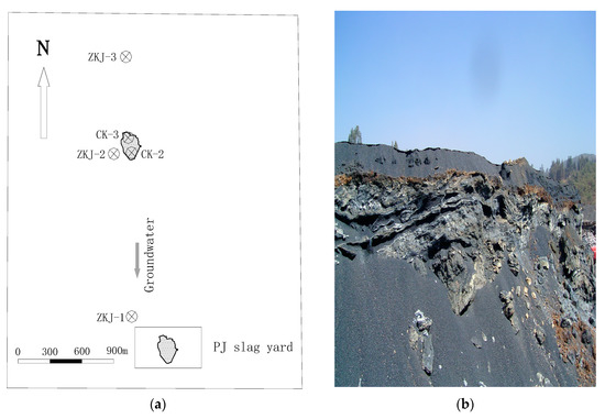
Figure 1.
View of the slag yard: (a) plan view of the slag yard and the five sampling locations and (b) a photo of a slope of the slag yard.
The hazardous materials in the slag yard included smelting slag and construction waste soil. Three samples of leaching solution from these materials were collected, according to the China criterion for identification of extraction toxicity [17] and were tested.
To obtain the real leaching water of rainfall in the slag yard, some perforated PVC tubes were made and buried in the bottom of the slag yard. Two samples of the real leaching water, from sampling sites CK-1 and CK-2 in Figure 1, were collected and tested.
Water quality near the slag field was collected and analyzed to evaluate the slag yard effects on surrounding groundwater. The groundwater sampling sites were ZKJ-1, ZKJ-2, and ZKJ-3, shown in Figure 1. Table 1 also lists the groundwater sampling sites. The water samples were obtained from the wells.

Table 1.
Concentration (C) of fluorine from the test results.
3. Results of the Experimental Investigation
The three samples of leaching solution from the hazardous matters were tested, and the concentration of fluorine in each sample is shown in Table 2. The test results showed that the concentrations of fluorine from smelting slag and construction waste soil all exceeded the discharge limit of 0.1 kg/m3 of the China criterion [18]. The test results also showed that the clay in the bottom of the slag yard absorbed some fluorine.
Table 2.
Concentration of fluorine.
The concentrations of fluorine in the leaching water samples from the slag yard after some days of rainfall are shown in Table 3. The test results showed that the concentrations were stable approximately 15 days after rainfall. The results also showed that the concentrations of fluorine were well over the World Health Organization (WHO) limit of 0.0015 kg/m3 in drinking water and the China health limit of 0.001 kg/m3 in drinking water [19].
Table 3.
Concentration of fluorine.
Table 1 shows the test results of the groundwater samples. The concentrations of fluorine did not reach the China health limit of 0.001 kg/m3 in drinking water.
The test results showed that the concentrations of fluorine from smelting slag and construction waste soil exceeded the discharge limit of 0.1 kg/m3 of the China criterion [18] and the concentrations of fluorine of the real leaching water of rainfall in the slag yard. Thus, fluorine was a contaminant, and it was necessary to study the scope of fluorine pollution of the slag yard.
4. Laboratory Studies of Solute Transport During Absorption of Water by Soil
The experimental studies of hydrodynamic dispersion of low concentration solutions during absorption into horizontal columns of soil were made for the clay under the slag yard. The main objective of these studies was to obtain the molecular diffusion coefficient of the clay for numerical simulation.
4.1. Theory for the Laboratory Studies
The conventional approach to hydrodynamic dispersion during one-dimensional water movement in soils involves the equation [20]:
in which C is the solute concentration in the water, θ is the volume fraction of fluid within the soil, q is the volume flux density of the solution, x is the space coordinate, t is time, and Dsh is the longitudinal dispersion coefficient.
The experiments were designed to realize the initial and boundary conditions:
In horizontal non-hysteretic systems, the flow of water may be described by the equations:
where D(θ) is the soil–water diffusivity.
Setting , the following equations are derived [20]:
It can be assumed that Dsh(θ) is a function principally of θ and that any dependence on q could be neglected. Thus, the following equations are used:
in which Dm is the molecular diffusion coefficient and θr is the residual water volume fraction of soil.
4.2. Tests and Results
Two clay samples designed to have the same dry bulk density as a clay sample in site were used for experiments. The test conditions are shown in Table 4. The main experiment results are shown in Figure 2, Figure 3 and Figure 4 and Table 5.
Table 4.
Test conditions.
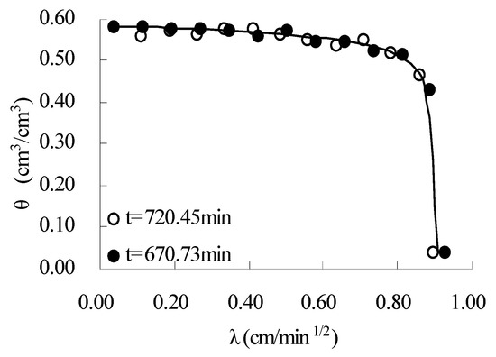
Figure 2.
The curves for relationship of θ-λ.
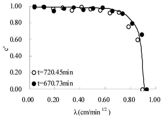
Figure 3.
The curves for relationship of C’-λ.
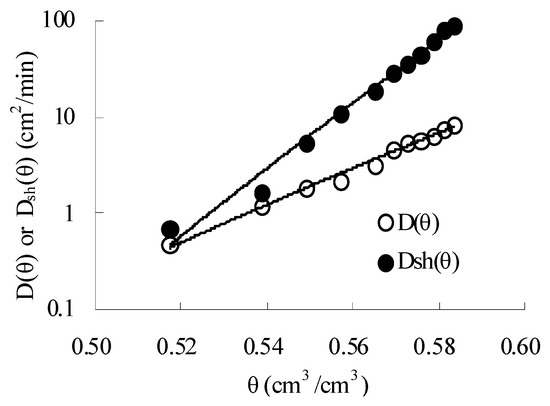
Figure 4.
Relationship curve of D(θ), Dsh(θ) and θ.
Table 5.
Test results.
5. Numerical Modelling Investigation
The fate and transport of pollution were simulated by COMSOL Multiphysics, which is a groundwater flow and solute transport visual software simulating the movement of solutes. Based on the program COMSOL Multiphysics, a model was built for solute transport in porous media, and the following equations were used in this model [21].
5.1. Fluid Flow
Richards’ equation governs the saturated–unsaturated flow of water in the soil. The soil air is open to the atmosphere, so it can be assumed that pressure change in air does not affect the flow. Here, Richards’ equation is used for single-phase flow. Richards’ equation can be expressed as:
where denotes the specific moisture capacity (m−1); Se is the effective saturation of the soil (dimensionless); S is a storage coefficient (m−1); Hp represents the dependent variable pressure head (m); K equals the hydraulic conductivity function (m s−1); E is the coordinate (for example, x, y, or z) that represents vertical elevation (m); and Qs is a fluid source defined by volumetric flow rate per unit volume of soil (s−1). In this equation, S = (θs − θr)/(1 m) where θs denotes the volume fraction of fluid under saturation.
For unsaturated flow, the fluid moves through the soil but may or may not completely fill the pores in the soil. The coefficients Ch, Se, and K vary with the pressure head, and Hp, together with θ, makes Richards’ equation nonlinear. The specific moisture capacity, Ch, relates the variations in soil moisture to pressure head as Ch = ∂θ/∂Hp. Because Ch, the first term in the time coefficient, goes to zero at saturation, time change in storage depends on the compression of the aquifer and water under saturated conditions. The saturated storage varies with the effective saturation, as represented by the second term in the time-coefficient. Furthermore, K is a function that defines how readily the porous media transmits fluid. The relative permeability of the soil, kr, increases with increasing fluid content given by K = Kskr, where Ks (m/s) is the constant hydraulic conductivity at saturation.
Groundwater flow and solute transport can be linked by fluid velocities. To follow the form of the transport equation, the fluid velocities need to be deduced from Darcy’s law:
5.2. Solute Transport
The equation that governs advection and dispersion is:
where DL is the hydrodynamic dispersion tensor and is referred to as Dsh(θ) in the preceding paragraph; Rk is the added solute per unit volume of water per unit time; and xi is the Cartesian coordinate. So, θDL in the three-dimensional case can be expressed as [20]:
5.3. Geological Model for the Hydrogeology Study in the Study Area
The ground layers were divided into six materials mainly based on their permeability difference, as follows [22]: material 1 was mainly composed of slag and construction waste soil; material 2 was clay; material 3 was unsaturated limestone located a certain distance away from groundwater; material 4 was saturated limestone within the scope of groundwater; material 5 was base rock with very low permeability; material 6 was sandy gravel. Material 3 and material 4 offered different permeability coefficients, which are shown in Table 6.
Table 6.
Model parameters for flow simulation.
Two simulation models based on exploratory boring are shown in Figure 5 and Figure 6 [22]. The 2D simulation model in Figure 5 was 10.462 km in length and 1.058 km in height and jointed by a lake. The 3D simulation model in Figure 6 was modelled by 8 profiles and was 1.840 km in length along the y direction, 0.89 km in width along the x direction, and 0.439 km in height. The layout of the ground layers was shown in Figure 5a,b and Figure 6a. Materials 1–4 of the 2D-model and the 3D-model were the same, but the 3D-model did not include material 5 because the 3D-model was shallower than the 2D-model.The 2D model was divided into 42,236 elements with 21,648 nodes, while the 3D model was divided into 67,968 elements with 14,620 nodes.
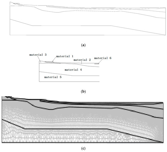
Figure 5.
2D compact numerical simulation model: (a) the whole geometric model; (b) the local geometric model, and (c) the finite element method model.
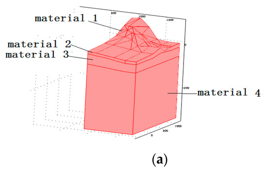
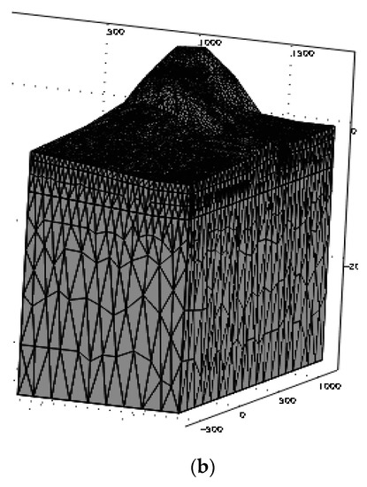
Figure 6.
3D compact numerical simulation model: (a) the whole geometric model and (b) the FEM model.
5.4. Boundary and Model Parameters for Flow Simulation
The seepage field must be simulated as accurately as possible to obtain reasonable simulation results of contaminant migration. Here, the seepage field was simulated as saturated–unsaturated stable seepage. For the model in Figure 5, the boundary conditions were set as follows [22]. The upper surface accepted rainfall infiltration and belonged to the flux boundary. The flux at the slag surface was 3.2 × 10⁻⁸ m/s, which was equal to the local average annual rainfall of 1012 mm. The flux at the clay surface was 1.6 × 10⁻⁹ m/s, which was 5% of the rainfall. The flux of the slag surfaces was 3.2 × 10⁻⁸ m/s because of the following reasons. First, the saturated permeability coefficients of the slag (0.0001 m/s and 0.0001 m/s) were very high so the rain water on the slag surface easily flowed into the slag and could be stored in the lower slag. Second, the clay surface under the slag was sunken so it could keep the water from the slag surface and some water from the clay surface. Finally, the water stored in the lower slag was covered by thick slag, so the evaporation of the rain water to atmosphere was very little. The flux of the clay surfaces was 1.6 × 10⁻⁹ m/s because of the following reasons. The saturated permeability coefficients of the clay were very low, so most of the rain water on the clay surface was easy to run off. Some of the water evaporated off, so the water penetration through clay surface would be very low. The two border surfaces vertical to the x-axis were set as boundaries with constant hydraulic head: one of the constant hydraulic heads was the hydraulic head in the exploratory hole; the other was the hydraulic head of the lake at the boundary. The bottom surface was set as a boundary with a constant flux of zero.
The seepage field of the 3D model in Figure 6 was also simulated as saturated–unsaturated stable seepage, and the following boundary conditions of seepage simulation were used [22]. The upper surface accepted rainfall infiltration, and the border belonged to flux boundary. The flux of the slag surfaces was 3.2 × 10⁻⁸ m/s while that of the clay surfaces was 1.6 × 10⁻⁹ m/s. The two border surfaces vertical to the x-axis were set as symmetric boundaries because they belonged to watersheds. The two border surfaces vertical to the y-axis were set as boundaries with constant hydraulic head: one was the hydraulic head in the exploratory hole on the boundary; the other was −61 m based on the simulation results of 2D FEM model. The bottom surface was set as a boundary with a constant flux of zero.
Soil–water characteristic curves for material 1 and material 2 were obtained from a volumetric pressure plate test, and the pore volume fractions were estimated from the corresponding soil–water characteristic curves. The residual water volume fractions for material 1 and material 2 were obtained from the drying method. The saturated permeability coefficients for material 1 and material 4 were estimated from a water injection test. Other parameters were determined according to the experience values in geotechnical engineering. All the saturated permeability coefficients of the materials, except those of material 2, are shown in Table 6 for simulation. The permeability coefficients of material 2 were important for determining the seepage field. Therefore, they were determined by inverse analysis based on the test results. Materials 1 and 2, whose soil–water characteristic curves were obtained from the test results, were set to be unsaturated materials. The soil–water characteristic curves of material 2 are shown in Figure 7, and the experimental curve of sample 82 was used for simulation. The test results indicated that the saturated permeability coefficient of material 2 in the vertical direction ranged from 5 × 10⁻⁹ m/s to 1 × 10⁻⁷ m/s. Simulation analysis showed that the simulation results of the seepage field could fit the actual seepage field better if the saturated permeability coefficient in the vertical direction was 8 × 10⁻⁸ m/s and that in the horizontal direction was 3 × 10⁻⁸ m/s.
Figure 7.
Soil–water characteristic curve for material 2.
5.5. Model Definition for Dissolved Solute Transport
The solute component identification test showed that the concentration value of fluorine in the slag solute was approximately 0.0045 kg/m3, while that of the solute on the clay surface was approximately 0.00005 kg/m3.
The following conditions were set for solute migration simulation. The initial value of slag solute was set to 0.0045 kg/m3, while that of other solutes were set to be 0.00005 kg/m3. Boundary conditions were as follows. Flux boundary was set to the upper surface of the model. The flux of the slag yard surfaces was (3.2 × 10−8) × 0.0045 kg m−2 s−1, while that of the clay surfaces was (3.2 × 10−8) × 0.00005 kg m−2 s−1. The concentration of fluorine in the water of the border surface with the higher constant hydraulic heads was set to 0.00005 kg/m3. The advective flux model was set to the border surface with the lower constant hydraulic heads. The flux of the bottom surface was zero. The fluxes of the two border surfaces vertical to the x-axis were set to be zero for the 3D FEM model.
The parameters of the materials used in the dispersion calculation are shown in Table 7. The molecular diffusion coefficient of material 2 was determined as Dm = 4.85 × 10⁻⁶ m2 s−1 based on the unsaturated dispersion test results shown in Table 5 and the clay saturation of survey results shown in Table 8. Other parameters, shown in Table 7, were determined according to the experience values in geotechnical engineering.
Table 7.
Model parameters for pollutant migration.
Table 8.
The clay saturation of survey results.
5.6. Results
Survey results showed that clay had a high saturation of approximately 0.95, as shown in Table 8. The simulation results of the 2D model showed that the saturation of clay near the slag in Figure 8 ranged from 0.89 to 0.95. The simulation results of the 3D model showed that the saturation of clay near the slag in Figure 8 ranged from 0.89 to 0.91. The saturation of clay near the slag in Figure 8 was approximately 0.9. The simulation results were consistent with survey results. The results of the calculations showed that the relative error between the simulation results and the survey results was less than approximately 10%. According to the Technical Requirements for Groundwater Numerical Simulation [23], a relative error below 10% is acceptable. Therefore, the formation model established for this study was feasible for the simulation.
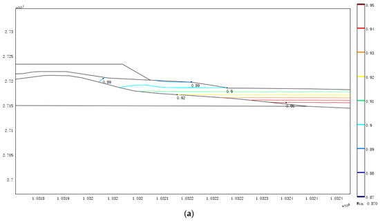
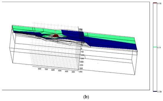
Figure 8.
Saturation contour in clay: (a) 2D model and (b) 3D model.
Groundwater quality near the slag field was analyzed to evaluate the slag field effects on the surrounding groundwater. Table 9 shows the groundwater sample test results and corresponding numerical simulation results. It can be seen that the numerical simulation results and test results are nearly identical. Hence, the numerical simulation results could be used as the basis of groundwater environment evaluation.
Table 9.
Comparison between test results and simulation results.
Figure 9 provides some solute migration simulation results of the 2D model. Over time, the solution with the fluorine concentration in the slag field migrated outward slowly. The dispersion velocity near the groundwater was so large that the fluorine concentration in the groundwater did not increase with time. The final fluorine concentration in the groundwater, 100 years after disposal started, did not exceed 0.001 kg m−3, which is the legislative upper limit of the second-grade water of China. The concentration in the groundwater did not exceed the legislative upper limit of the second-grade water of China. The maximal pollution water range, from the slag yard to the south, 52 years after disposal started, was approximately 123 m, and was approximately 172 m 100 years after disposal started.
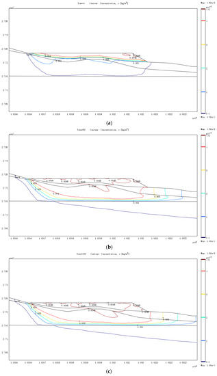
Figure 9.
Simulated concentration contour of fluorine in groundwater of the situation of the neighboring slag yard of 2D model: (a) 1 year after disposal started, (b) 52 years after disposal started, and (c) 100 years after disposal started.
Figure 10, Figure 11 and Figure 12 provide some solute migration simulation results of the 3D model. Over time, the solution with the fluorine concentration in the slag field migrated outward slowly. The dispersion velocity near groundwater was so large that the fluorine concentration in the groundwater did not increase with time. The final fluorine concentration in the groundwater 100 years after disposal started did not exceed 0.001 kg m−3. The concentration in the groundwater did not exceed the legislative upper limit of the second-grade water of China. The maximal pollution water range, from the slag yard to the south, 52 years after disposal started, was approximately 185 m, and the range 100 years after disposal started was approximately 330 m. The maximal pollution water range, from the slag yard to the west, 52 years after disposal started, was approximately 75 m, and the range 100 years after disposal started was approximately 135 m. The maximal pollution water range, from the slag yard to the east, 52 years after disposal started, was approximately 60 m and the range 100 years after disposal started was approximately 80 m.
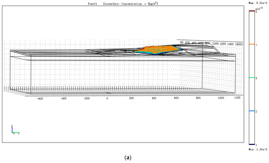
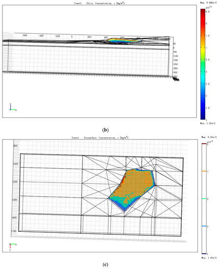
Figure 10.
Simulated concentration contour of fluorine in groundwater of 3D model 1 year after disposal started: (a) the overall situation, (b) the situation of a typical profile, and (c) the situation of plan view.
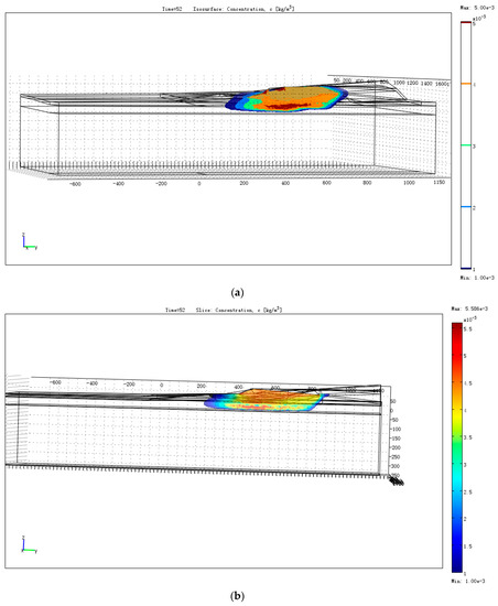
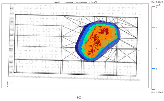
Figure 11.
Simulated concentration contour of fluorine in groundwater of 3D model 52 years after disposal started: (a) the overall situation, (b) the situation of a typical profile, and (c) the situation of plan view.
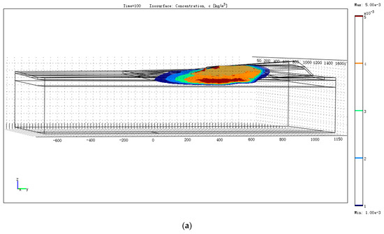
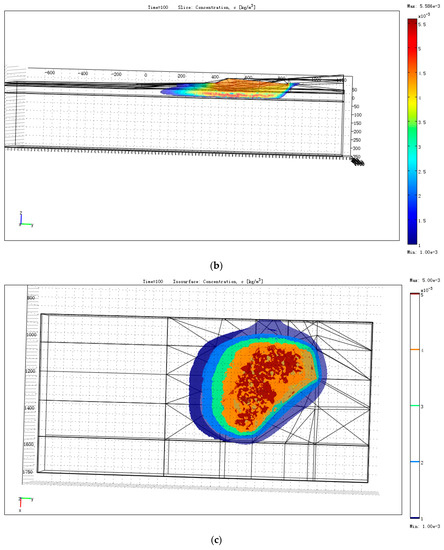
Figure 12.
Simulated concentration contour of fluorine in groundwater of 3D model 100 years after disposal started: (a) the overall situation, (b) the situation of a typical profile, and (c) the situation of plan view.
5.7. Discussion
Comparing to the study in the literature, a large-scale three-dimensional numerical simulation of groundwater fluoride concentration was performed, and the maximal fluoride pollution water range was attempted to be determined based on a large-scale three-dimensional numerical simulation of groundwater fluoride concentration for the first time.
5.8. Limitations
The limitation of this study was that the sorption of fluoride in clay and the mineralogical sources of groundwater fluoride from the matters out of the slag were not considered. The fluorine concentrations would be less if the sorption of fluoride in clay and the mineralogical sources of groundwater fluoride from the matters out of the slag were considered [16].
6. Conclusions
In this paper, a large-scale three-dimensional numerical simulation method to investigate the fluorine pollution near a slag yard was implemented. The large-scale three-dimensional numerical simulation method included experimental investigation, laboratory studies of solute transport during absorption of water by soil, and a large-scale three-dimensional numerical simulation of solute transport. Experimental investigations were performed, and the test results showed that the concentrations of fluorine from smelting slag and construction waste soil exceeded the discharge limit of 0.1 kg/m3 of the China criterion. The key parameters of the materials used for numerical simulation were determined based on the experimental investigation, the laboratory studies, the soil saturation of survey results, and back analyses. A large-scale two-dimensional numerical simulation and a large-scale three-dimensional numerical simulation of solute transport were implemented, and their results were compared to the experimental results. The following conclusions were made.
(1) The simulation results showed that the clay near the slag had high saturation of approximately 0.9, which was consistent with survey results.
(2) Comparison of the results showed that the numerical simulation results of solute transport and test results were basically identical. Thus, the numerical simulation results could be used as the basis of groundwater environment evaluation.
(3) Over 100 years of simulation, the pollution plume from the slag field migrated outward slowly. The dispersion velocity near the groundwater was so large that the fluorine concentration in the groundwater did not increase with time. The final fluorine concentration in the groundwater 100 years after disposal started did not exceed 0.001 kg m−3, the legislative upper limit of the second-grade water of China. The maximal pollution water range from the slag yard to the south, 52 years after disposal started, was approximately 185 m, and the range 100 years after disposal started was approximately 330 m. The maximal pollution water range from the slag yard to the west, 52 years after disposal started, was approximately 75 m. The range 100 years after disposal started was approximately 135 m. The maximal pollution water range from the slag yard to the east, 52 years after disposal started, was approximately 60 m, and the range 100 years after disposal started was approximately 80 m.
To compare with the study in the literature, a large-scale three-dimensional numerical simulation of groundwater fluoride concentration was performed, and the maximal fluoride pollution water range was attempted to be determined based on a large-scale three-dimensional numerical simulation of groundwater fluoride concentration for the first time.
Author Contributions
Conceptualization, L.W.; methodology, L.W.; validation, L.W. and S.S.; formal analysis, L.W.; investigation, L.W. and S.S.; resources, S.S.; data curation, L.W. and S.S.; writing—original draft preparation, L.W.; writing—review and editing, L.W.; visualization, L.W.; supervision, C.W.; project administration, C.W.; funding acquisition, S.S.
Funding
This research was funded by the National Natural Science Foundation of China, grant number 51074152.
Acknowledgments
The author would like to thank for the help from project (51074152) supported by National Natural Science Foundation of China and the help from the project supported by Kunming Prospecting Design Institute of China Nonferrous Metal Industry.
Conflicts of Interest
The authors declare no conflict of interest.
References
- Arnesen, A.K.M.; Krogstad, T. Sorption and desorption of fluoride in soil polluted from the aluminum smelter at Ãrdal in western norway. Water Air Soil Pollut. 1998, 103, 357–373. [Google Scholar] [CrossRef]
- Ayoob, S.; Gupta, A.K. Fluoride in drinking waters: A review on the status and stress effects. Crit. Rev. Environ. Sci. Technol. 2006, 36, 433–487. [Google Scholar] [CrossRef]
- Wang, L.F.M.; Huang, J.Z. Outline of control practice of endemic fluorosis in China. Soc. Sci. Med. 1995, 41, 1191–1195. [Google Scholar] [PubMed]
- Mjengera, H.; Mkongo, G. Appropriate deflouridation technology for use in flourotic areas in Tanzania. Phys. Chem. Earth 2003, 28, 1097–1104. [Google Scholar] [CrossRef]
- Voss, C.I. A Finite-Element Simulation Model for Saturated-Unsaturated, Fluid Density-Dependent Groundwater Flow with Energy Transport or Chemically-Reactive Single-Species Solute Transport; Water-Resources Investigations Report, 84-4369; U.S. Geological Survey: Reston, VA, USA, 1984.
- Nishigaki, M.; Hishiya, T.; Hashimoto, N.; Kohno, I. The numerical method for saturated-uns- aturated fluid-density-dependent groundwater flow with mass transport. J. Geotech. Eng. 1995, 501, 135–144. [Google Scholar]
- Sonnenthal, E.; Ito, A.; Spycher, N.; Yui, M.; Sugita, Y.; Conrad, M.; Kawakami, S. Approaches to modeling coupled thermal, hydrological, and chemical processes in the drift scale heater test at Yucca Mountain. Int. J. Rock Mech. Min. Sci. 2005, 42, 698–719. [Google Scholar] [CrossRef]
- Nawa, N.; Miyazaki, K. The analysis of saltwater intrusion through Komesu underground dam and water quality management for salinity. Paddy Water Environ. 2009, 7, 71–82. [Google Scholar] [CrossRef]
- Sikdar, P.K.; Chakraborty, S. Numerical modelling of groundwater flow to understand the impacts of pumping on arsenic migration in the aquifer of north bengal plain. J. Earth Syst. Sci. 2017, 126, 29–50. [Google Scholar] [CrossRef]
- Berger, T.; Mathurin, F.A.; Drake, H.; Åström, M.E. Fluoride abundance and controls in fresh groundwater in Quaternary deposits and bedrock fractures in an area with fluorine-rich granitoid rocks. Sci. Total Environ. 2016, 569–570, 948–960. [Google Scholar] [CrossRef] [PubMed]
- Datta, P.S.; Deb, D.L.; Tyagi, S.K. Stable isotope (18O) investigations on the processes controlling fluoride contamination of groundwater. J. Contam. Hydrol. 1996, 24, 85–96. [Google Scholar] [CrossRef]
- Halletta, B.M.; Dharmagunawardhaneb, H.A.; Atalc, S.; Valsami-Jonesd, E.; Ahmedc, S.; Burgessa, W.G. Mineralogical sources of groundwater fluoride in Archaen bedrock/regolith aquifers: Mass balances from southern India and north-central Sri Lanka. J. Hydrol. Reg. Stud. 2015, 4, 111–130. [Google Scholar] [CrossRef]
- Olaka, L.A.; Wilke, F.D.; Olago, D.O.; Odada, E.O.; Mulch, A.; Musolff, A. Groundwater fluoride enrichment in an active rift setting: Central Kenya Rift case study. Sci. Total Environ. 2016, 545–546, 641–653. [Google Scholar] [CrossRef] [PubMed]
- Rafique, T.; Naseem, S.; Ozsvath, D.; Hussain, R.; Bhanger, M.I.; Usmani, T.H. Geochemical controls of high fluoride groundwater in Umarkot Sub-District, Thar Desert, Pakistan. Sci. Total Environ. 2015, 530–531, 271–278. [Google Scholar] [CrossRef] [PubMed]
- Zabala, M.E.; Manzano, M.; Vives, L. Assessment of processes controlling the regional distribution of fluoride and arsenic in groundwater of the Pampeano Aquifer in the Del Azul Creek basin (Argentina). J. Hydrol. 2016, 541, 1067–1087. [Google Scholar] [CrossRef]
- Wei, L. Study Report of Experiment of Soil and Numerical Simulation of Groundwater Pollution of the Copper Slag Yard in Puji; Institute of Rock and Soil Mechanics of Chinese Academy of Sciences: Wuhan, China, 2011. (In Chinese) [Google Scholar]
- GB5085.3-2007. Identification Standards for Hazardous Wastes and Identification for Extraction Toxicity; China Environmental Science Press: Beijing, China, 2007. [Google Scholar]
- GB 8978—1996. Integrated Wastewater Discharge Standard; Standards Press of China: Beijing, China, 1996. [Google Scholar]
- GB/T14848–93. Quality Standard for Ground Water; Standards Press of China: Beijing, China, 1993. [Google Scholar]
- Smiles, D.E.; Philip, J.R. Solute transport during absorption of water by soil: Laboratory studies and their practical implications. Soil Sci. Soc. Am. J. 1978, 42, 537–544. [Google Scholar] [CrossRef]
- COMSOL, A.B. The COMSOL Multiphysics Reference Guide; COMSOL Office: Stockholm, Sweden, 2008. [Google Scholar]
- Wei, L. Study on Migration and Pollution in Shallow Groundwater Near a Slag Field. J. Residuals Sci. Tech. 2015, 12, 191–197. [Google Scholar] [CrossRef]
- GWI-D1. Technical Requirements for Groundwater Numerical Simulation; Standards Press of China: Beijing, China, 2004. [Google Scholar]
© 2019 by the authors. Licensee MDPI, Basel, Switzerland. This article is an open access article distributed under the terms and conditions of the Creative Commons Attribution (CC BY) license (http://creativecommons.org/licenses/by/4.0/).