On the Nature of Pressure Wave Propagation through Ducts for Structural Health Monitoring Application

Abstract

An effective structural health monitoring system fully exploits the flexibility offered by the 3D printing process by integrating a smart structural health monitoring technology inside the 3D-printed components. The system relies on the propagation of pressure waves with constant propagation speed through circular capillaries embedded in the structure. The nature of these waves seems to be determinant for the accuracy of the crack localization system. To achieve a better physical understanding of the nature of the propagating waves through the capillaries, computational fluid dynamics simulations are performed and compared to experimental results obtained with a self-built test setup. The presence of propagating shock waves is observed in the simulations and experiments, as well as a complex reflection mechanism around the leak location. Shock waves show the characteristic of not propagating at a constant velocity. This property complicates the actual localization system. To solve this, the constant velocity assumption should be replaced with the effective velocity evolution to increase the localization accuracy. The amplitude of the shock wave is attenuated with propagating distance, which proves that the effect of friction plays an important role and can, in turn, influence the localization system.

1. Introduction: Crack Localization Based on Pressure Wave Propagation

1.1. Additive Manufacturing

Metal Additive Manufacturing (AM), more commonly known as 3D metallic printing, introduces the “imagination is the limit” concept in the manufacturing. 3D printing is a promising technology with maximum design freedom. Building layer by layer, the technique prints components with highly complex geometries from almost any digital model. Therefore, the determining factor for the cost of the component switches from its complexity to its size and/or the amount of material used. However, the technique shows an important structural drawback [1,2,3]. Both the fatigue behavior and residual stresses of the component are modified in a negative way.

1.2. Structural Health Monitoring

To overcome this hurdle and mitigate the risk, strategies must be developed for the detection and localization of manufacturing defects in the 3D-printed components. A critical element in aeronautics non-destructive testing is the detection of the presence of a crack before it reaches a critical size. Similar important issues retarded the introduction of lightweight composite materials in aeronautics. To prevent the same difficulties with the introduction of 3D metal-printed light-weight components in aeronautics and in many other applications, it is important to invest significant research efforts into the measurement of the structural health of the component under operation conditions. The academic community has proposed several Structural Health Monitoring (SHM) techniques in the last decade [4,5,6]. Many of these approaches work well in laboratory conditions, but are not able to detect damage in a sufficiently effective manner and are not robust enough to be applied in practice. A high detection probability and the avoidance of false alarms are essential for a proper operation of the system, as well as background noise reduction. One major aspect that is often overlooked is the lifetime of the monitoring system itself and its robustness with respect to the operational environmental conditions [7,8]. All these reasons show the importance of dedicating substantial research efforts to structural health monitoring methodologies to detect and localize cracks in the 3D-printed parts of tomorrow.

1.3. Effective Structural Health Monitoring

Considering the advantages and drawbacks of structural health monitoring systems, a new effective Structural Health Monitoring (eSHM) system has been developed [9,10]. With the proposed eSHM methodology, the flexibility offered by the 3D printing process can be fully exploited to integrate the smart monitoring technology inside the 3D-printed components. The eSHM system is based on the detection of pressure changes in 3D-curved capillaries (see the red channels in Figure 1) that are integrated in the component thanks to additive manufacturing techniques. The capillary channels can be compared with the human nervous system, in which the pain receptors of the body inform the brain by sending signals to it. It is crucial to embed the capillaries in the fatigue critical regions of the component. By using a vacuum pump, the capillaries are set initially at a very low pressure (quasi-vacuum). After the structure has been fatigue loaded, cracks can be initiated and will then propagate through the structure. If the crack encounters a capillary on its way, contact occurs between the atmosphere and the low-pressure volume inside the capillary. Due to the pressure difference between both volumes, the sudden crack-capillary contact induces the propagation of pressure waves through the capillary channel towards both ends. These waves are monitored by two pressure probes (S1,S2) located at both ends of the capillary. As shown in Equation 1, by exploiting the difference in the time of arrival $t_2-t_1$ of the front wave at both ends of the duct, the location of the crack $x_1$ w.r.t S1 can be retrieved. This principle currently relies on the constant propagation speed characteristic of acoustic pressure waves (= speed of sound), for which a value of $c=340$ m/s is considered.

$$x_1=\frac{L-c(t_2-t_1)}{2}$$

(1)

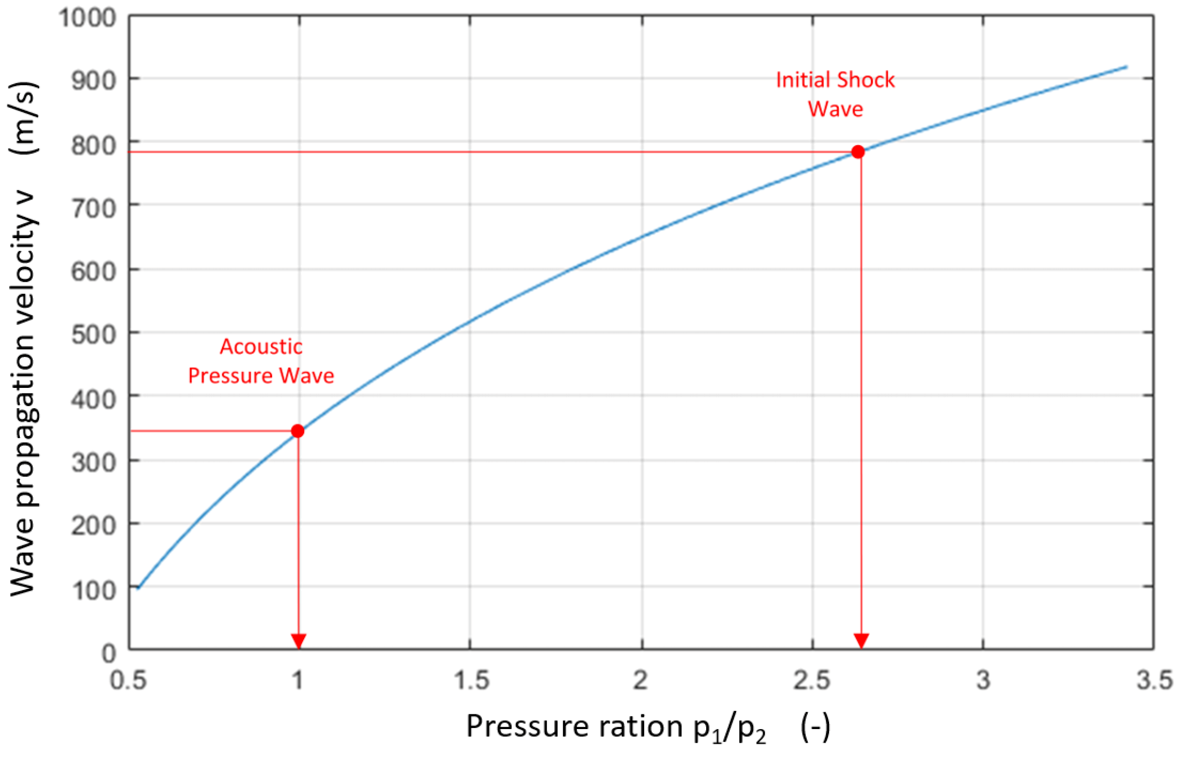
1.4. Nature of Pressure Wave Propagation

The exact nature of the propagating waves does not seem to be completely identified in the available literature. The pressure difference measured by the sensors can be of a hydrodynamic, acoustic, or hydro-acoustic nature depending on the moment of acquisition and measurement conditions. The suddenness of the opening, as well as the pressure difference between atmospheric conditions (in the crack) and low-pressure conditions (in the capillary) seem to be determinant. Depending on their nature, these pressure waves could be defined as acoustic pressure waves (acoustic phenomenon) [11] or shock waves (fluid dynamics phenomenon) [12].

Acoustic pressure waves (also called negative pressure waves in some references) have been deeply studied in the past in both gaseous and liquid media to retrieve the location of cracks in large-scale pipelines [13,14]. Pipelines are one of the most secure methods to deliver oil and gas. The potential risk of leaks in the pipeline should be lowered as much as possible for environmental and safety reasons. In some particular cases, the losses can even become detrimental for the performance of the installation. Here again, the localization principle relies on the constant propagation speed characteristic of the propagating wave. The only difference w.r.t. the eSHM-system is the scale of the pipelines in terms of length and diameter. Analytically, the acoustic pressure waves are described by the isentropic linearized Navier–Stokes equations. These waves are associated with small pressure changes and result in a zero net mass flow. Their propagation speed corresponds to the local speed of sound, and after their passage, the state of the medium stays unchanged. This process is adiabatic, reversible, and keeps the entropy constant. The acoustic linearized shock tube model [15] can be used as a reference to described the phenomenon.

On the other hand, considering different initial conditions, shock waves can travel through the capillary at a speed higher than the local speed of sound in the medium. These waves are defined as a sudden irreversible discontinuity in pressure, density, and temperature of the fluid and are associated with violent pressure changes. Shock waves give a change in entropy and are described by the non-linear Navier–Stokes equations. Their passage is non-adiabatic and abruptly changes the state of the medium in an irreversible way. The main difference with the acoustic pressure waves is their non-constant propagation speed and the net mass flow behind the shock after its passage. Propagating shock waves are not a common topic in the literature. In the case of detached bowed and oblique shocks around moving bodies, as well as in converging-diverging nozzles, the shock is considered in a fixed position and the fluid is moving. However, when a balloon is bursting, an atomic bomb is exploding, or in turbocharged internal combustion engines, the shock wave propagates through a stationary medium. The theoretical shock tube model [16] used in the field of gas dynamics can be compared to the phenomenon happening in the capillaries. This model describes the phenomenon happening in a tube divided into two different pressure zones (high-pressure zone and low-pressure zone), just after the sudden burst of a thin diaphragm. The burst creates a shock wave propagating further through the lower pressure zone of the duct. The removal of the diaphragm can be compared with the moment where the crack reaches the capillary. In his work, Parisse [17] presented the analysis of this shock wave propagation through small-scale ducts. The presence of shock waves would complicate the localization technique since their propagation speed theoretically depends on the amplitude, in contrast to the acoustic pressure waves where the propagation speed is constant. The next equation highlights the amplitude dependency of the propagation speed [18]:

$$v=a\pm \frac{\gamma +1}{2}u=a\left(1\pm \frac{\gamma +1}{\gamma -1}\left({\left(\frac{p_1}{p_2}\right)}^{\frac{\gamma -1}{1}}-1\right)\right)$$

(2)

In which a is the speed of sound, u the velocity behind the wave, $\gamma$ the heat capacity ratio, and $p_1/p_2$ the ratio of the pressure before and after the wave. As shown in Figure 2, in the case of an acoustic pressure wave, the pressure ratio equals one, the equation is reduced to $v=a$, and the wave travels at the speed of sound (see the red dot in Figure 2). On the other side, shock waves propagate at a speed higher or equal to the speed of sound depending on their amplitude ($p_1/p_2$). Based on the pressure difference considered in the present study, the initial propagation speed of the shock wave theoretically equals 788 m/s (see the red dot in Figure 2).

Acoustic pressure waves can be seen as a limiting case of shock waves. Particular shock diffusive weakening effects [19,20] can decrease the shock amplitude till reaching $p_1/p_2=1$. The small scale of the duct increases the relative importance of the friction, and the viscous stresses tend to deform the wave front. With propagation distance, a boundary layer develops behind the shock (called shock–boundary layer interaction), and its thickness could become important w.r.t. the duct diameter. The smoothing of the shock results in an attenuation of both the velocity and pressure jump over the shock. These reasons could give a plausible explanation for the lower accuracy and some unclarified observations for small-scale measurements presented in the work of Hinderdael et al. [11]. Further, the observed pressure jumps in [11] suggest an irreversible behavior similar to the shock wave feature. Therefore, the present study focuses on the nature of the propagating waves to clarify matters.

1.5. Objectives and Methodology

The purpose of this work is to achieve a better physical understanding of the nature of the waves propagating through the capillaries. First, a numerical study is realized in which the flow through the leak is simulated by means of computational fluid dynamics simulations. As a second step, these results are compared to measurements obtained using a self-built experimental setup. The specificities of the present work are highlighted in the next points:

• Previous experiments described in [10,11] were performed on short ducts of around $L=0.5$ m. In this work, longer ducts of $L=3$ m are considered. In this way, a deeper understanding of the propagation behavior of the wave can be obtained. Next to that, it allows analyzing if the system can be used for larger components, where the effect of friction could become important due to the longer length of the capillaries and therefore influence the wave propagation speed and localization accuracy.
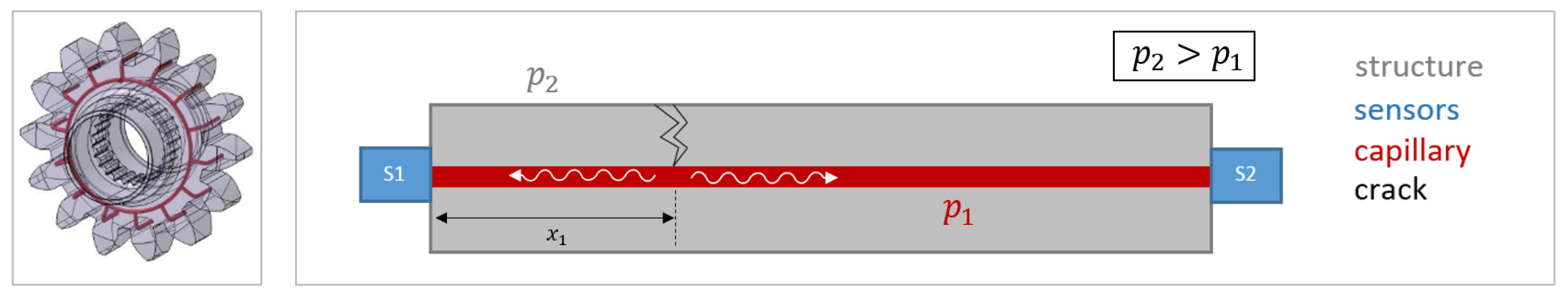
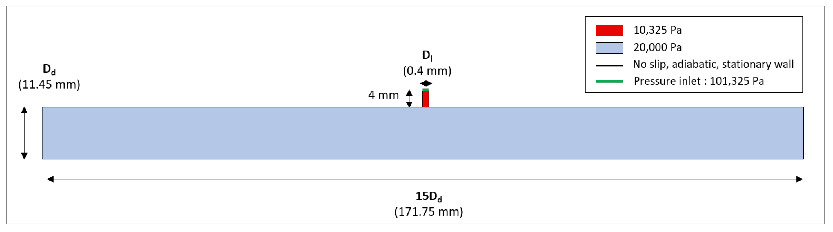
• The diameter and location of the capillary channels is of high importance in terms of structural integrity of the part. The inclusion of capillaries in the structure reduce its resistance and should as a consequence be optimized to the smallest possible dimension. Considering a trade-off between the actual 3D printing accuracy and the structural integrity of the component, the capillary diameter should not exceed $1.6$ mm. For practical reasons, in the present study, a duct diameter of $D_d=11.45$ mm is considered. In this way, the physics behind the problem can be understood without having to tackle the difficulties implied by the real small-scale dimensions. As highlighted before, the wave propagation through larger scale ducts is also widely used for pipeline leak detection; see [21]. Therefore, this work will address research questions that are relevant for both leak localization techniques (small and large scale). According to Rocha’s equation [22] for choked flow, the diameter ratio $D_{leak}/D_d$ is the only geometrical parameter affecting the amplitude of the propagating wave:

  $$\Delta P=0.37P_{atm}{\left(\frac{D_{leak}}{D_d}\right)}^2$$

  (3)

  in which $P_{atm}$ represents the static atmospheric pressure condition in the leak. To obtain the same amplitude in this study as for the real application with capillary channels, the diameter ratio is set at the same value; see Equation (4). The pressure jump of the wave is expected to equal $\Delta P\approx 36$ Pa; see Equation (3). More information about the geometry is given in Section 2.1.1.

  $${\left(\frac{D_{crack}}{D_{cap}}\right)}_{real}={\left(\frac{D_{leak}}{D_d}\right)}_{study}=0.003$$

  (4)

2. Numerical Study: Physical Understanding of Wave Propagation Mechanism

The goal of these simulations is to gain a better physical insight into the acoustic/shock wave generation and propagation. Next to that, the development of a numerical tool will allow the analysis of the effect of relevant parameters at a later stage. 2D computational fluid dynamics simulations were performed using the commercial software Fluent 19.0 (ANSYS, Canonsburg, PA, USA).

2.1. Numerical Parameters

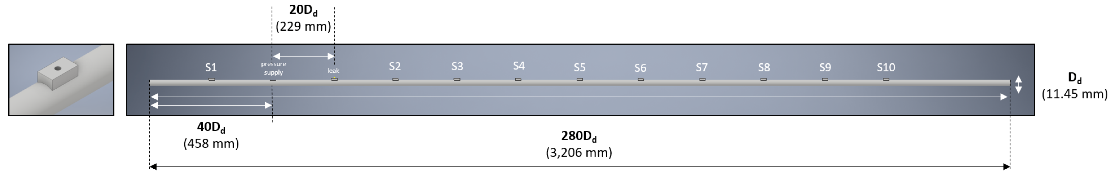
2.1.1. Geometry

The main duct had a diameter of $D_d=11.45$ mm and was $15D_d$ long; see Figure 3. The focus was set on a short region around the crack to allow observing the propagation and reflection mechanism of the wave around the leak location without reaching too long computation times. Experimentally speaking, measuring close to the leak would involve a few difficulties. The leak was located in the middle of the axial length of the duct. The expected crack size in fatigue-loaded metallic components corresponded to $D_{crack}=50$ μm. In order to respect the same diameter ratio (4) for both simulations and real-life applications (as explained in Section 1.5), the leak diameter was chosen as $D_{leak}=0.4$ mm.

2.1.2. Initial and Boundary Conditions

The density-based solver (with absolute velocity formulation) was used because of its higher accuracy in terms of shock resolution compared to the pressure-based solver. The density-based solver automatically includes the viscous dissipation terms in the energy equation. Since one deals with compressible flow, the energy equation was activated. Air was used as the fluid with ideal gas properties, and other properties were kept constant. A pressure-inlet was defined at the entrance of the leak and was set at atmospheric conditions. In order to reproduce the real initial conditions in the best way, the numerical pressure inside the duct was initialized at 20 kPa and the leak at atmospheric conditions at $101.3$ kPa. To finish, a zero (no-slip) velocity and adiabatic condition were applied on all the walls.

2.1.3. Solution Methods

The laminar viscous model was used, and no turbulence model was applied. Since the first-order upwind scheme may tend to smooth the shocks, the second-order upwind flow discretisation was used. For the gradient spatial discretisation scheme, the least squares cell-based option was selected. The first-order implicit formulation was used as the transient formulation and is considered sufficient for most problems. Finally, the AUSM (Advection Upstream Splitting Method) was chosen as the convective flux type since it provides an exact resolution of contact and shock discontinuities and is recommended for such cases. The time-step of the transient simulation was set at $5\times {10}^{-10}$ s.

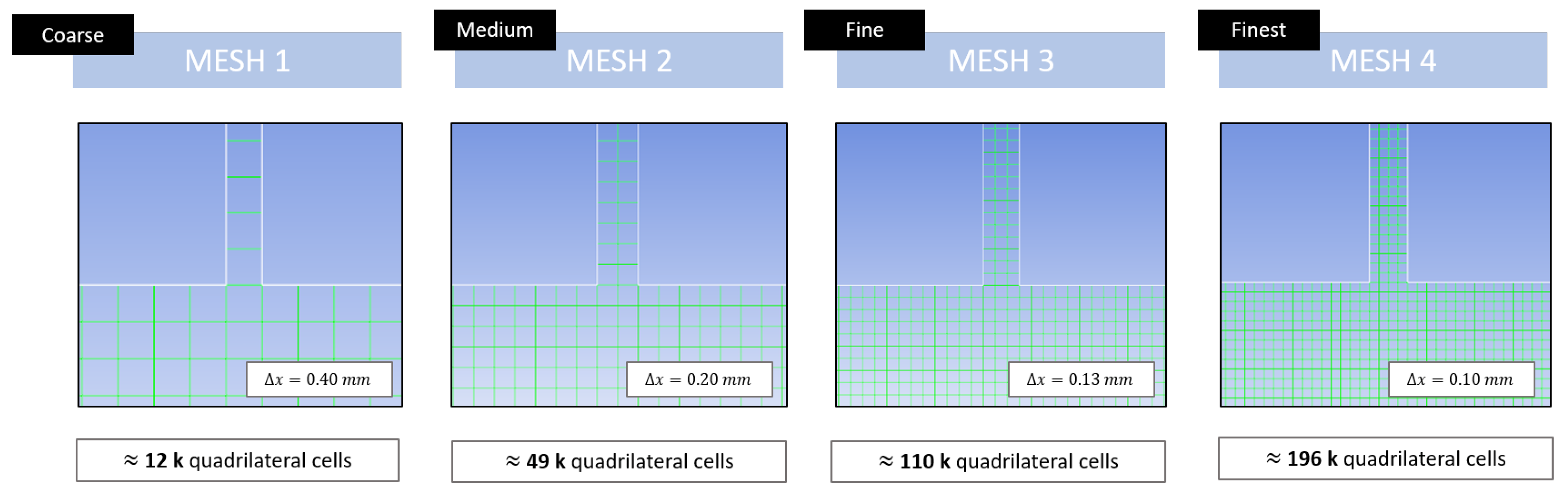
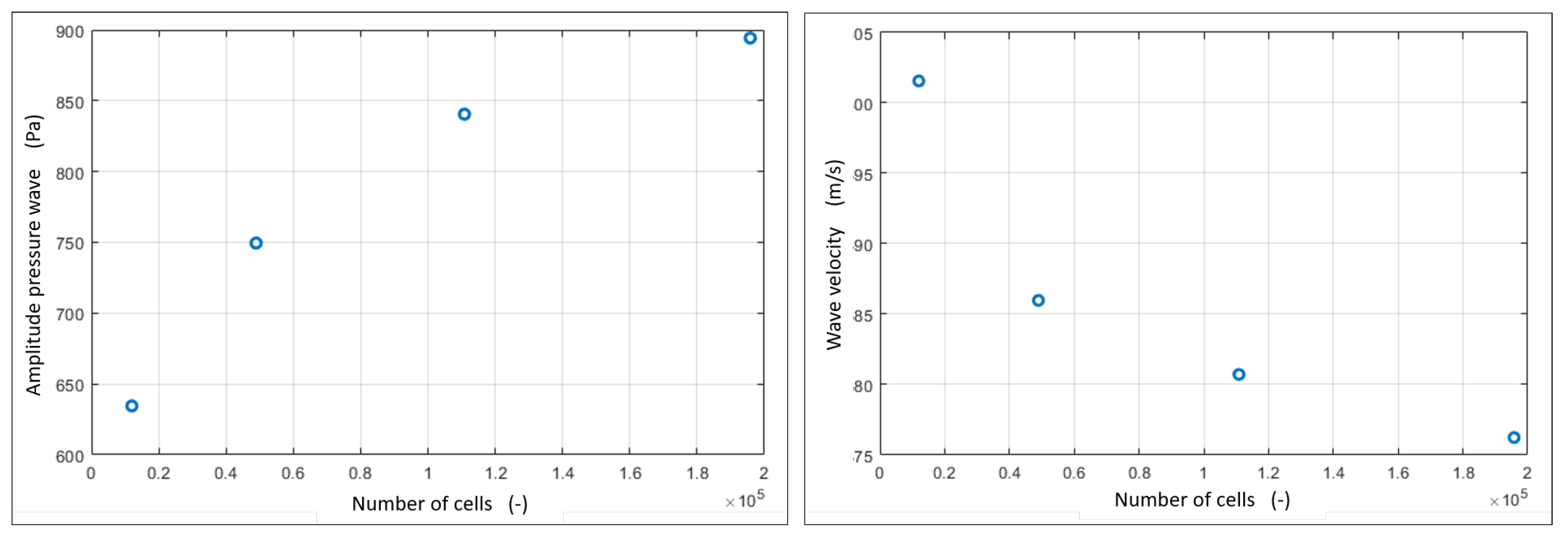
2.1.4. Grid Convergence Study

The convergence of the result to the exact solution in terms of wave propagation speed and wave amplitude was crosschecked by performing a grid convergence study on four different meshes. The meshes were created using the Gambit meshing software and are composed of respectively 12 k, 49 k, 110 k, and 196 k quadrilateral cells. As can be seen in Figure 4, giving detailed views of the meshes, respectively 1, 2, 3, and 4 elements were considered over the leak width. The same cell size was used over the complete mesh. The cell size $\Delta x=\Delta y$ is defined in Figure 4 for each of the cases and had a direct influence on the accuracy of the shock arrival time and therefore on the wave propagation speed. At a duct axial distance $1.7D_d$ of the leak position, this resulted in a maximum error of $\delta v=7.8,3.9,2.6$, and $1.9$ m/s going from the coarse mesh to the finest mesh. Obviously, this error on the velocity reduced with propagation distance from the leak position.

The following graphs in Figure 5 give the amplitude of the wave and the wave velocity for an increasing number of cells. The data of both graphs were extracted for a propagation distance of flow time $t=5.14\times {10}^{-5}$ s corresponding to a $1.7D_d$ propagation distance of the wave from the leak position. The same tendency was obtained at any flow time or propagation distance. The wave velocity was computed by considering the first rise in pressure as wave arrival. According to Rocha’s equation in 2D, the amplitude of the wave should equal $1.3$ kPa. Refining the mesh brought the amplitude closer to the theoretical value, but a relative error of 30% was still observed.

The main differences in the solution between the four refinements are the smoothness of the shock, resolution of the shock front, and the correct description of the flow behavior close to the leak. Clearly, the finest mesh gave a much sharper shock front, and therefore allowed locating the shock front and the wave velocity with higher accuracy. The wave velocity evolved to an asymptotic value of 372 m/s (considering a power fit) for an increasing number of cells. Consequent extra refinement would be needed to get a slight improvement of the velocity accuracy and would therefore significantly increase the computation time. These reasons explain why the finest mesh was chosen as the final grid refinement. It is important to notice that the high refinement of the duct induced high computation times. Since the length of the duct was determinant for the computational cost of the simulation, the geometry was cut into two, and a symmetry boundary condition was added on the axial centerline of the leak. This reduced the computational time by around $50\%$ and would allow simulating longer duct lengths.

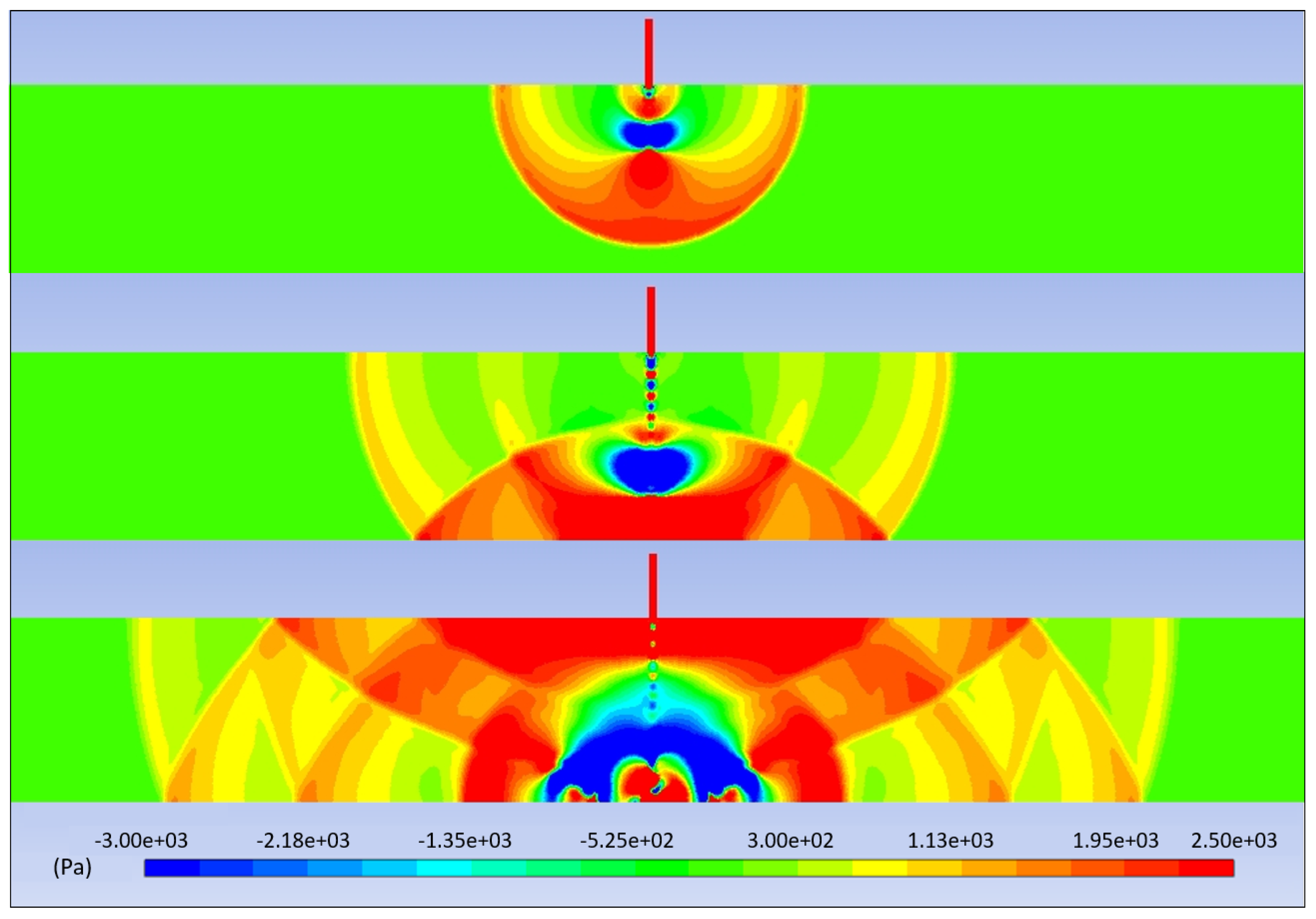
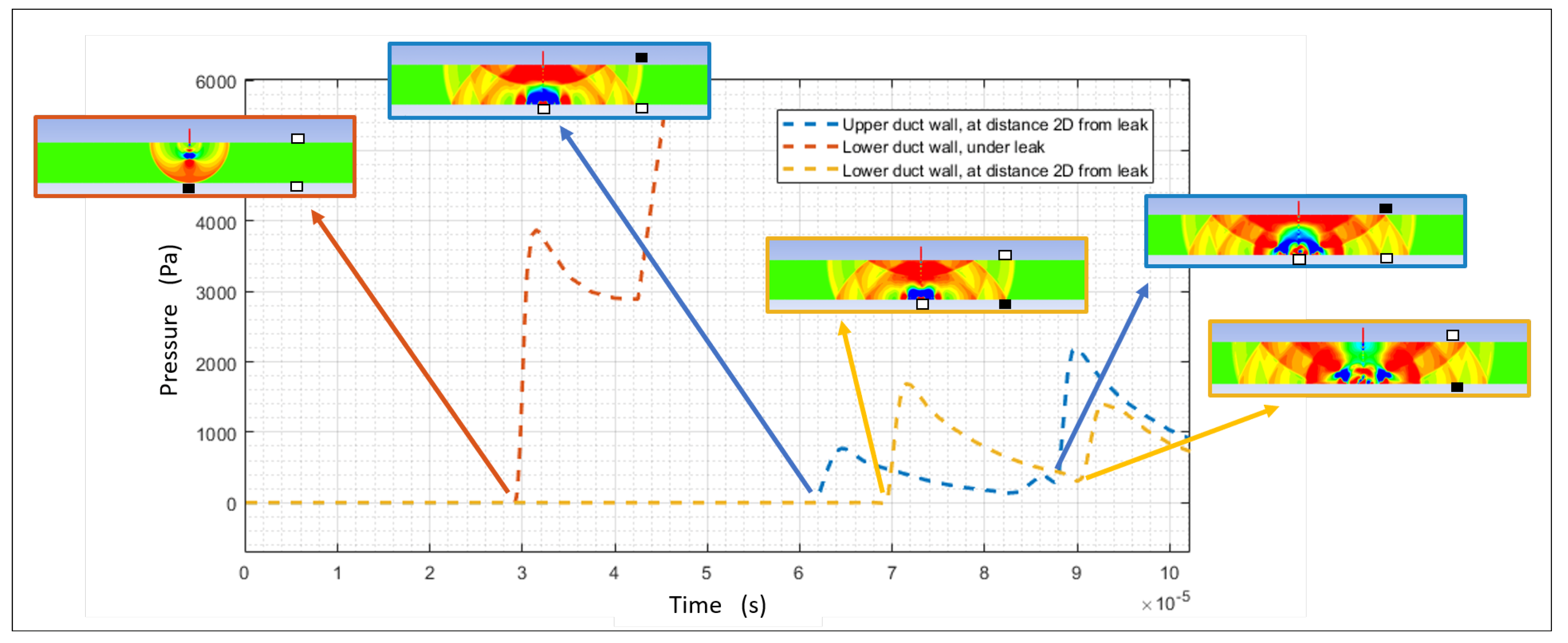
2.2. Results: Shock Wave Propagation Visualization

The propagation of the shock wave is shown in the static pressure contour plots given in Figure 6. Cell values were used to avoid discontinuity so as to be smeared graphically by node averaging. A shock wave is a discontinuity created when a disturbance propagates at a faster speed than the speed of sound in a fluid. This abrupt discontinuity changes the characteristics of the medium and gives rise to irreversible pressure changes in the fluid. The same behavior is observed in the given contour plots.

First, a small spherical shock can be seen as a centered energy source was created at the contact between the leak and the duct. This shock expanded spherically, dissipated energy (leading to a decrease in amplitude and propagation speed), and traveled till reaching the lower duct wall. At the lower wall, a hard wall shock wave reflection created a new increase in pressure and amplification of the shock strength. The strong shock produced after reflection propagated faster towards both ends of the duct and had a higher amplitude than the incident shock front. This can be explained by the fact that the passage of the first shock increased the velocity of the medium in which the reflected shock would propagate. The reflected shock front would therefore propagate through a medium that was already in motion and catch up with the first shock front with propagation distance. Both waves collapsed together and formed a Mach stem reflection on the lower wall of the duct. The Mach stem intensity was twice as high as the incident shock front [15]. This was observed on the contour plot since the static pressure value of the shock front at the lower wall (where the Mach stem was formed) was higher w.r.t. the upper wall. After a certain propagation distance, the combination of these effect created a complex reflection mechanism (see $t_3$ in Figure 6. To finish, the presence of a supersonic localized jet with so-called diamond shocks was observed at the exit of the leak. The diamonds were stationary and would not travel through the capillary, and were therefore not important for this study. The propagation of the first shock front can therefore be considered as a phenomenon on its own, since it was not influenced by the filling of the duct due to the jet. It was observed that the flow velocity close to the leak was not increasing in the first instance. Meanwhile, the shock front was created and propagated further without any influence of the incoming flow. Only after the shock wave passage (local irreversible perturbation), the jet started to fill the capillary, and the flow velocity increased. It was concluded that only the behavior of the first shock front, which evolved from a spherical shock front to a normal shock front with traveling distance, was important for the present application.

The shock front pressure amplitude at the upper duct wall was extracted at different axial locations and is shown in the left plot of Figure 7 together with a power curve fit on the data (a fit type that resulted in the highest $R^2$ value). The leak is located at $x=0$ mm. A lowering of the amplitude with traveling distance was observed, and it evolved to an asymptotic value of 300 Pa. The shock wave carried energy that dissipated with traveling distance due to viscosity. It is known that shock waves are much more sensitive to viscous weakening effects in comparison to acoustical pressure waves. According to [15], the shock–boundary layer interaction implies a lowering of the shock wave amplitude and propagation speed. In the right plot of Figure 7, the propagation velocity of the first shock front was computed based on the arrival time and distance traveled by the shock. As expected, the wave propagation speed showed the same decreasing behavior as for the amplitude (see Equation (2)). The velocity evolved to an asymptotic value of 347 m/s. This shows that the shock wave behavior (propagation speed > speed of sound) tended to go back to the acoustic pressure wave behavior (propagation speed = speed of sound) with propagation distance. The change in wave velocity observed in the $15D_d$-length region around the leak would complicate the localization system if one of the sensors were located too close to the leak location. This is a plausible explanation for the remaining localization error in the experiments of Hinderdael et al. [10] since they assumed constant propagation speeds in small length ducts. Therefore, both sensors should be placed far enough from the critical fatigue zone where cracks can occur or the localization method should be adapted taking into account the non-constant velocity evolution of the wave in order to be applicable in any situation. When employed as a leak detection principle for long pipelines, this shock wave behavior around the leak with non-constant propagation speed is clearly less important than for the eSHM-system. Due to the longer propagation distance, the non-constant behavior of the velocity close to the leak will be averaged out.

In Figure 8, the shock front pressure is extracted at different locations along the duct walls as a function of time. The locations at which the pressure is extracted over time are indicated with a black cube on the corresponding pressure contour plots. The red curve gives the first pressure jump measured by the imaginary sensor located on the lower wall of the duct, just under the leak position. Later, the second pressure step was measured on the upper wall of the duct at a distance $2D_d$ from the leak position (see blue curve). Finally, due to the curved shape of the shock front, the third pressure jump (yellow curve) was measured around $1\times {10}^{-5}$ s later w.r.t the blue curve. The pressure jump in blue did not undergo any reflection before being measured. This explains why its amplitude was lower than for the red and yellow pressure jumps. The red pressure jump had a higher amplitude since it was measured just at the hard wall reflection location. With traveling distance, the amplitude of the shock front lowered due to friction with the wall. The increasing surface of the spherical shock after its reflection under the leak location was also responsible for the amplitude decrease. The shock started at the leak location as a point of energy. This energy was then distributed over the expanding surface of the shock front. For the blue and yellow curves, a second pressure jump was observed at a later time. These jumps are identified in the corresponding contour plots as being the reflections of the shock arriving later at the sensor locations.

3. Experimental Study: Validation of Simulations and Quantification Effect of Friction

The experimental campaign was realized to validate the observations of the CFD simulations and to verify if the shock wave attenuated over a long propagation distance. In terms of numerics, this analysis would require a too important computational cost due to the long length of the duct.

3.1. Setup Description

An experimental setup was built to measure the shock wave pressure jump at different propagation distances from the leak; see Figure 9. To simulate the sudden contact between the leak and the duct, a fast switching FESTO (Esslingen am Neckar, Germany) MHE2-MS1H valve was connected to a metallic piece in which a cylindrical hole with a reference diameter of $D_l=0.4$ mm was drilled. In this way, the opening time and location of the leak were known and controlled. The leak simulator was placed at a distance of $60D_d$ from the left end of the duct. The pressure tank was connected to the duct at a distance pf $40D_d$ from the left end side. Ten different measurement spots were equally distributed over the length $L=280D_d$ of the duct with a spacing of $20D_d$. One measurement spot was located to the left of the leak and the others on the right-hand side.

Ten Endevco Meggitt 8530C-50 pressure sensors simultaneously measured the pressure inside the duct while their signal was sent to the LMS (Leuven, Belgium) Scadas III mobile data acquisition system and visualized using the Spectral Testing software (LMS, Belgium, Leuven). The data processing was realized using MATLAB (MathWorks, Natick, MA, USA). To obtain flush mounted sensors w.r.t. the inner wall of the duct (to avoid any non-desired shock reflections), steel blocks with the same height as the sensor tips were welded on the outer part of the duct; see Figure 9 (left side). Both ends of the duct were closed by the welding of steel cylinders. The final experimental setup in the laboratory can be seen in Figure 10.

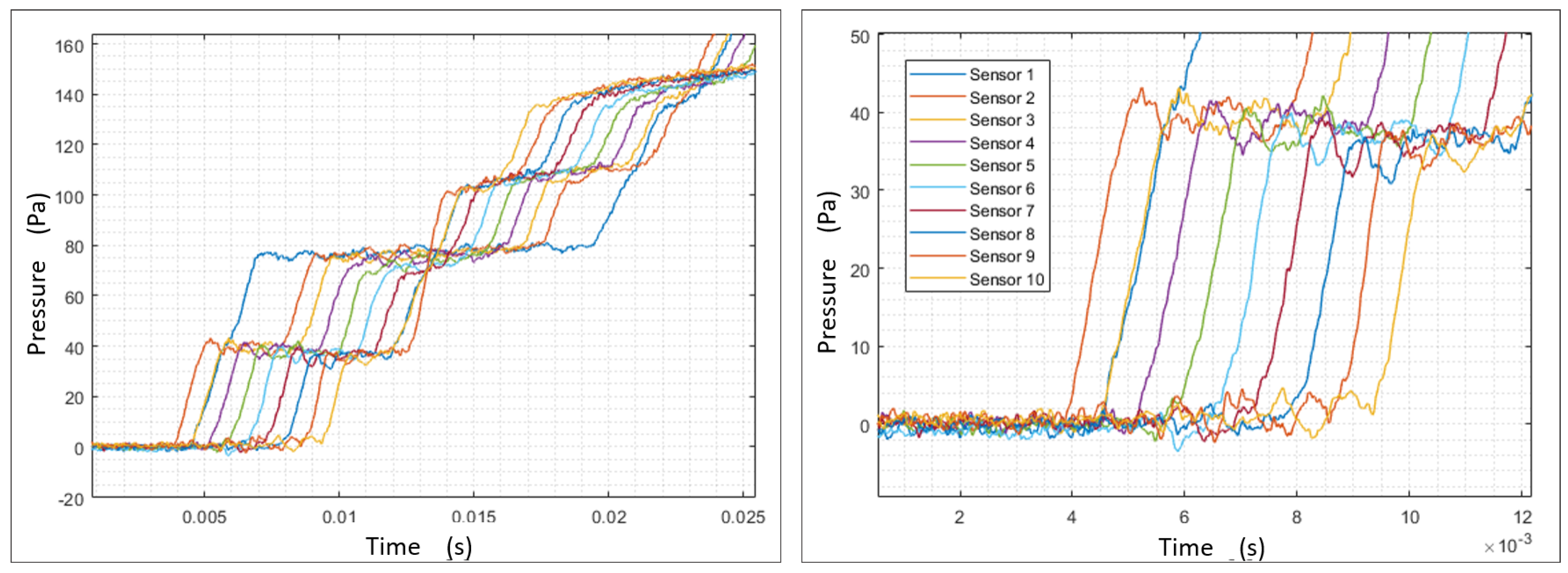
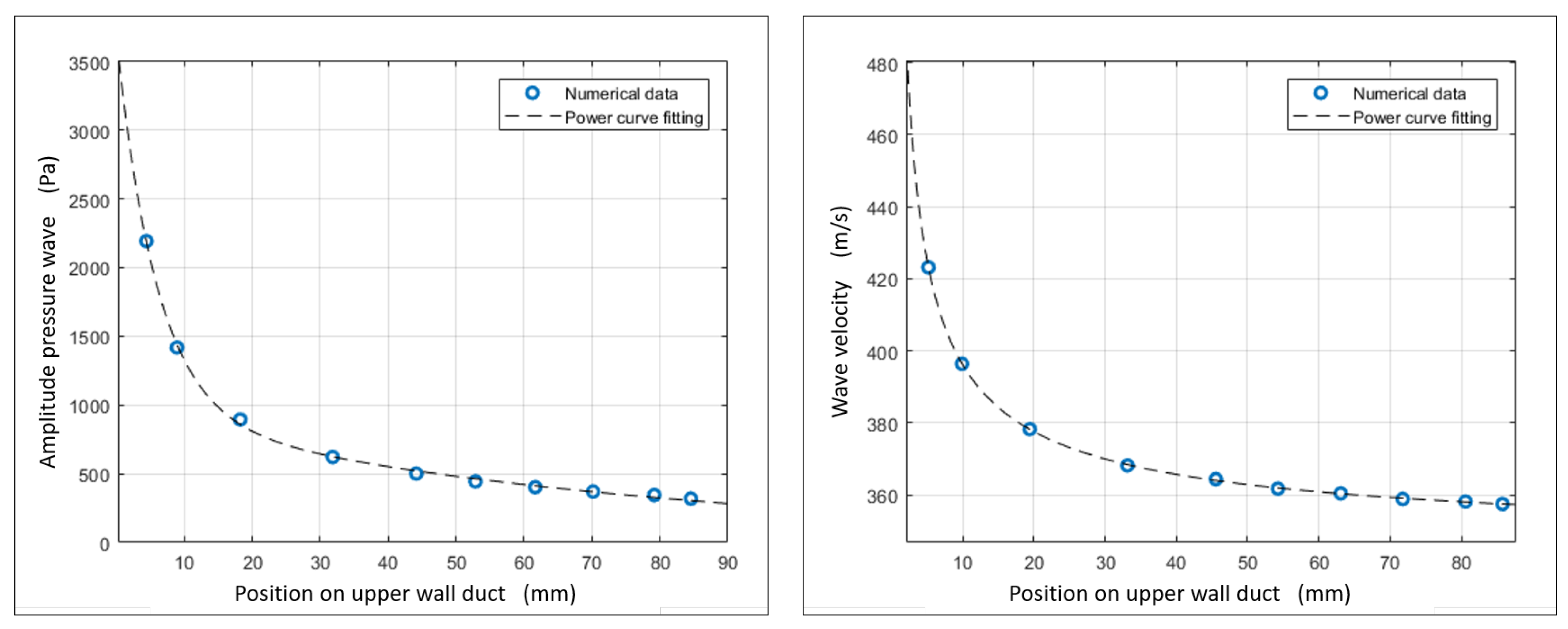
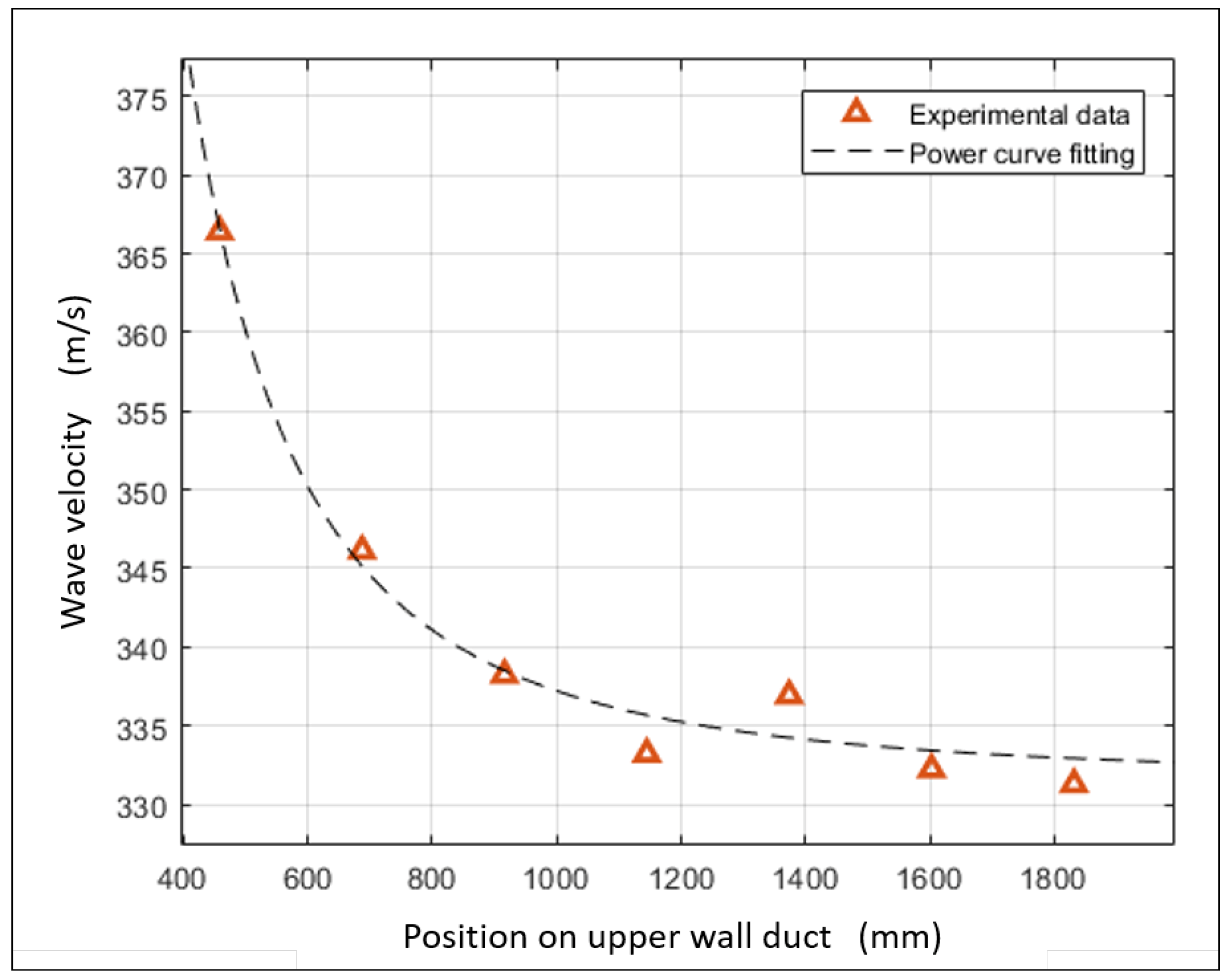
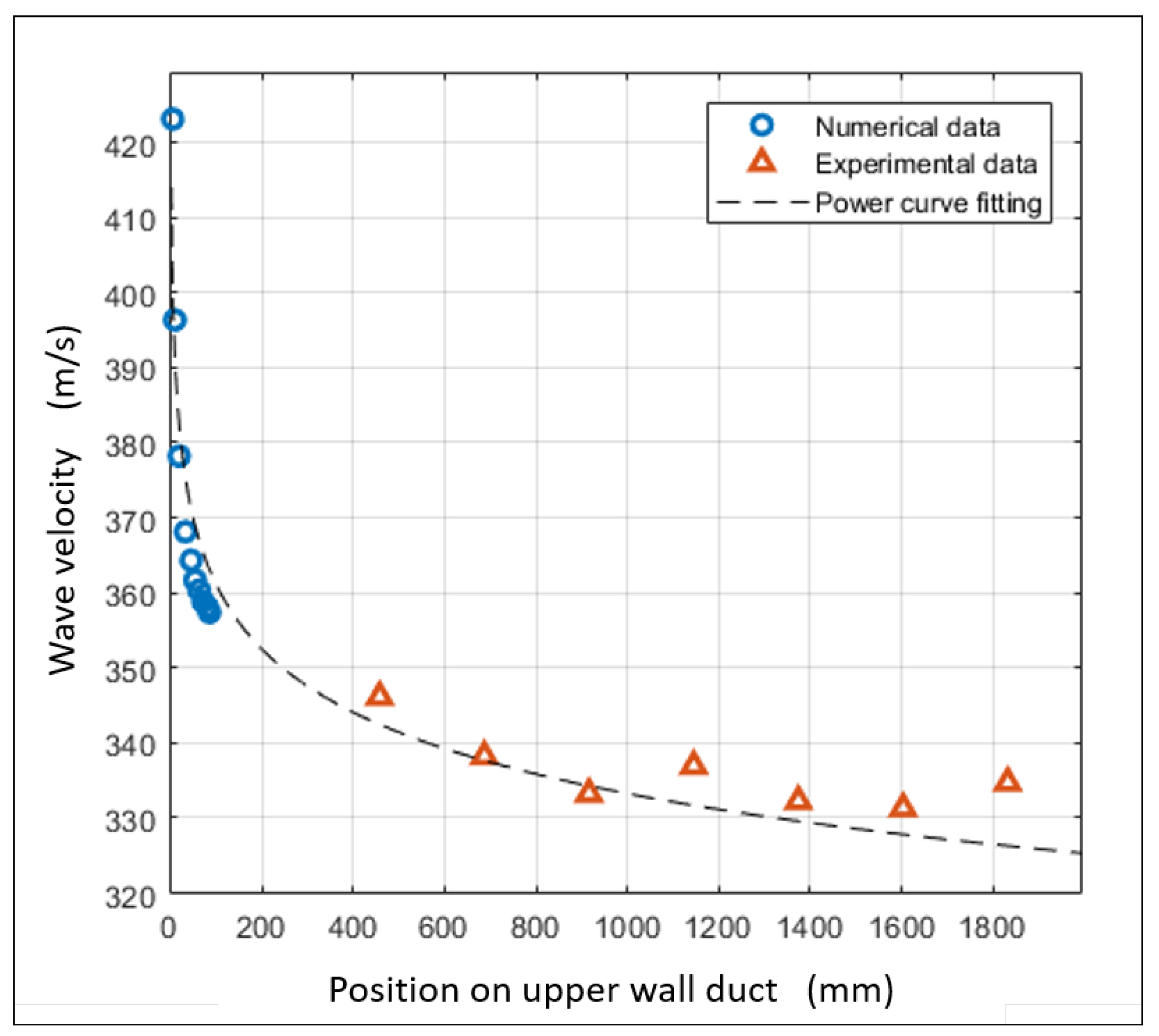
3.2. Results: Shock Wave Pressure Jump Observation

The signal was digitally filtered (zero-phase digital filtering, $f_c=5$ kHz) and the measurement repeated 10 times and averaged in order to improve the signal-to-noise ratio. Figure 11 gives the measurement of the pressure jump at the ten different locations on the duct. As expected, Sensor 2 (located closest to the leak) measured the pressure jump first. Afterwards, both Sensors 1 and 3 measured the pressure jump at the same moment since they were both located at the same distance $40D_d$ from the leak. The same reasoning can be applied for the other sensors. After the first shock front arrival, consequent pressure steps were observed for the 10 sensors. Hinderdael et al. showed in their work [11] that the pressure steps represent the reflections of the waves on the hard end walls of the duct. The information needed for the localization of the leak resides only in the first shock front arrival; therefore, a zoom of the first pressure step is shown on the right of Figure 11.

The amplitude measured at Sensor 2 reached 43 Pa. A difference of 7 Pa was observed compared to the theoretical expected value of 36 Pa (≈20% relative error on the amplitude), computed based on Equation 3. As was the case for the simulations, an amplitude decrease (≈6 Pa) was observed between Sensors 2 and 10. This resulted in a decrease in amplitude due to the friction between the shock wave and the solid surface of $3.3$ Pa/m. Note that this amplitude cannot be compared to the simulations, which were performed in 2D. After filtering, the maximum peak-to-peak noise corresponded to $3.7$ Pa. Considering this, shock wave reflections (with an amplitude higher than average noise on the signal) were identified after the first shock front arrival. This shows a similar behavior as the one highlighted in the simulations.

The experimental wave propagation velocity is given in Figure 12. To obtain an accurate arrival time of the wave, a polynomial curve fitting was applied over the curve slopes of Figure 11. The moment of wave arrival was defined as the moment at which the polynomial fit exceeded the maximum noise on the signal. The measurement points on the graph corresponded to Sensors 3–10 located on the right-hand side of the leak. Sensor 1 was located on the left-hand side and is therefore not shown. In turn, Sensor 2 is not depicted in the plot since it was used as a reference point to compute the wave velocities. Due to the inconsistency of the valve dynamics, it gave a more accurate result for the velocity (since the moment at which the wave passed at the location of Sensor 2 was known). The velocity evolved to an asymptotic value (≈333 m/s) close to the speed of sound.

For both simulations and experiments, a decrease in velocity was observed with propagation distance. Quantitatively however, differences were noted. It is important to remark that the length scales considered for the numerical simulations and the experiments were different. In Figure 13, both numerical and experimental results are shown. A simulation domain of $L=15D_d$ around the leak was chosen to avoid excessive computational times. On the other hand, it was difficult to experimentally measure in the region close to the leak. This is why an experimental duct length of $L=280D_d$ was chosen. Next to that, it also allowed observing the effect of viscosity for long propagation distances. A power curve fitting over the complete data is given in the plot (the fit type that resulted in the highest $R^2$ value). The same tendency of decreasing propagation speed was observed for both cases. This change in wave propagation velocity complicates the localization system and should therefore be taken into account for the localization.

4. Conclusions

We conclude that the shock wave behavior and a complex reflection mechanism were observed around the leak location in both numerical and experimental studies. The propagation of shock waves close to the leak induced the amplitude dependency of the propagation speed. The friction reduced the shock amplitude and velocity with propagation distance, and they evolved to asymptotic values. This shows that the shock wave behavior tends to go back to a more simple acoustic pressure wave behavior for increasing propagation distance. The shock wave behavior will be more pronounced in real-life applications for small-scale capillaries. First, their length will be smaller to be integrated in the additive manufactured parts, and secondly, the duct’s inner surface-to-volume ratio is higher; therefore, the effect of friction is more pronounced. These reasons complicate the localization system and are the reasons why a lower accuracy was obtained in previous experiments. Some care should be taken with the location of the sensors that cannot be placed in a region too close to the leak (to avoid the measurement of these local phenomena). To improve the accuracy of the localization, the real velocity evolution should be taken into account instead of the previous constant propagation speed assumption. According to the experimental results, the effect is less important for pipeline leak detection applications where long ducts are considered. The small amplitude of the measured waves (due to the small leak dimensions) combined with their attenuation with propagation distance could make their detection critical for long narrow capillaries.

5. Future Work

To investigate the quantitative differences between experimental and numerical simulations, it is necessary to switch to 3D turbulent simulations where initial forces become dominant w.r.t. the viscous forces. To improve the numerical cost, especially in the case of studies on longer ducts, a dynamic gradient adaptation has to be applied. To achieve a deeper understanding of the shock behavior, an extra experimental campaign with sensors located closer to the leak is being run. The experimental visualization of the shock behavior by means of the Schlieren technology would also be an asset. Once the problem is experimentally validated and can be simulated efficiently, the effect of different capillary shapes and configurations, duct roughness parameters, etc., will be possible without the need for additional experiments.

References

1. Gorelik, M. Additive manufacturing in the context of structural integrity. Int. J. Fatigue 2017, 94, 168–177. [Google Scholar] [CrossRef]
2. Molaeia, R.; Fatemi, A. Fatigue Design with Additive Manufactured Metals: Issues to Consider and Perspective for Future Research. In Proceedings of the 7th International Conference on Fatigue Design, Senlis, France, 29–30 November 2017. [Google Scholar]
3. Lia, C.; Liua, Z.Y.; Fangb, X.Y.; Guo, Y.B. Residual Stress in Metal Additive Manufacturing. In Proceedings of the 4th CIRP Conference on Surface Integrity, Tianjin, China, 11–13 July 2018. [Google Scholar]
4. Hou, Q.; Jiao, W.; Ren, L.; Cao, H.; Song, G. Experimental study of leakage detection of natural gas pipeline using FBG based strain sensor and least square support vector machine. J. Loss Prev. Process Ind. 2014, 32, 144–151. [Google Scholar] [CrossRef]
5. Boller, C.; Meyendorf, N. State-of-the-Art in Structural Health Monitoring for Aeronautics. In Proceedings of the International Symposium on NDT in Aerospace, Fürth/Bavaria, Germany, 3–5 December 2008. [Google Scholar]
6. Ciang, C.C.; Lee, J.R.; Bang, H.J. Structural health monitoring for a wind turbine system: A review of damage detection methods. Meas. Sci. Technol. 2008, 19, 122001. [Google Scholar] [CrossRef]
7. Kessler, S.S.; Amaratung, K.; Wardle, B.L. An assessment of Durability Requirements for Aircraft Structural Health Monitoring Sensors. In Proceedings of the 5th International Workshop on Structural Health Monitoring, Stanford, CA, USA, 12–14 September 2005; pp. 812–819, ISBN 1-932078-51-7. [Google Scholar]
8. Speckmann, H.; Henrich, R. Structural Health Monitoring (SHM)—Overview on technologies under development. In Proceedings of the 6th WCNDT 2004—World Conference on NDT, Montreal, QC, Canada, 30 August–3 September 2004. [Google Scholar]
9. De Baere, D.; Stranza, M.; Hinderdael, M.; Devesse, W.; Guillaume, P. Effective Structural Health Monitoring with Additive Manufacturing. In Proceedings of the EWSHM 7th European Workshop on Structural Health Monitoring, La Cité, Nantes, France, 8–11 July 2014. [Google Scholar]
10. Hinderdael, M.; de Baere, D.; Guillaume, P. Proof of Concept of Crack Localization using Negative Pressure Waves in closed tubes for later application in effective SHM system for Additive Manufactured Components. Appl. Sci. 2016, 10, 33. [Google Scholar] [CrossRef]
11. Hinderdael, M.; Jardon, Z.; de Baere, D.; Devesse, W.; Guillaume, P. Negative Pressure Wave Amplitude: A Theoretical Model Empirically Validated. J. Hazard. Mater. 2007, submitted. [Google Scholar]
12. Mirshekari, G.; Brouillette, M. One-dimensional model for microscale shock tube flow. Shock Waves 2009, 19, 25–38. [Google Scholar] [CrossRef]
13. Liang, W.; Zhang, L.; Wang, Z. State of research on negative pressure techniques applied to leak detection in liquid pipelines. In Proceedings of the International Pipeline Conference, Volumes 1, 2, and 3, Calgary, AB, Canada, 4–8 October 2004. [Google Scholar] [CrossRef]
14. Silva, R.; Buiatti, C.M.; Cruz, S.L.; Pereira, J.A.F.R. Pressure wave behaviour and leak detection in pipelines. Comput. Chem. Eng. 1996, 20 (Suppl. 1), S491–S496. [Google Scholar] [CrossRef]
15. Ben-Dor, G.; Igra, O.; Elperin, T. Volume 2: Shock wave interactions and propagation. In Handbook of Shock Waves; Academic Press: Cambridge, MA, USA, 2000; ISBN-13 978-0120864300. [Google Scholar]
16. Gaetani, P.; Guardone, A.; Persico, G. Shock tubes flows past partially opened diaphragms. J. Fluid Mech. 2008, 602, 267–286. [Google Scholar] [CrossRef]
17. Parisse, J.D.; Giordano, J.; Perrier, P.; Burtschell, Y.; Graur, I.A. Numerical investigation of micro shock waves generation. Microfluid. Nanofluid. 2009, 6, 699–709. [Google Scholar] [CrossRef]
18. Liepmann, H.W.; Roshko, A. Elements of Gasdynamics; Dover Publications Inc.: Mineola, NY, USA, 2002; ISBN-13 978-0486419633. [Google Scholar]
19. Zeitoun, D.E.; Burtschell, Y.; Graur, I.A.; Ivanov, M.S.; Kudryavtsev, A.N.; Bondar, Y.A. Numerical simulation of shock wave propagation in microchannels using continuum and kinetic approaches. Shock Waves 2009, 19, 307–316. [Google Scholar] [CrossRef]
20. Ngomo, D.; Chaudhuri, A.; Chinnayya, A.; Hadjadj, A. Numerical study of shock propagation and attenuation in narrow tubes including friction and heat losses. Comput. Fluids 2010, 39, 1711–1721. [Google Scholar] [CrossRef]
21. Murvay, P.S.; Silea, I. A survey on gas leak detection and localization techniques. J. Loss Prev. Process Ind. 2012, 25, 966–973. [Google Scholar] [CrossRef]
22. Rocha, M.S. Acoustic Monitoring of Pipeline Leaks; ISA: Amsterdam, The Netherlands; London, UK, 1989; pp. 283–290, no. 89-0333. [Google Scholar]
Figure 1. (Left) Cogwheel with integrated capillaries. (Right) Schematics of the effective SHM (eSHM) system.
Applsci 09 00837 g001
Figure 2. Wave propagation velocity evolution as a function of wave amplitude p 1 / p 2 .
Applsci 09 00837 g002
Figure 3. Initial and boundary conditions.
Applsci 09 00837 g003
Figure 4. Detailed views of the meshes for mesh dependency analysis.
Applsci 09 00837 g004
Figure 5. Grid convergence study: (Left) wave pressure amplitude; (right) wave velocity.
Applsci 09 00837 g005
Figure 6. Shock wave visualization of the 2D simulation: static pressure contour plot at, respectively, t 1 = 9 × 10 5 s, t 2 = 5 × 10 5 s, and t 3 = 4 × 10 5 s.
Applsci 09 00837 g006
Figure 7. (a) Wave amplitude evolution with propagation distance. (b) Wave propagation velocity evolution with propagation distance.
Applsci 09 00837 g007
Figure 8. Pressure-time plot at different locations through the duct with corresponding static pressure contour plots of 2D simulation.
Applsci 09 00837 g008
Figure 9. Experimental setup dimensions.
Applsci 09 00837 g009
Figure 10. Experimental setup for wave propagation observation.
Applsci 09 00837 g010
Figure 11. Pressure–time measurement at different upper duct wall locations.
Applsci 09 00837 g011
Figure 12. Wave velocity evolution with propagation distance.
Applsci 09 00837 g012
Figure 13. Comparison of numerical and experimental results.
Applsci 09 00837 g013