Optical Helicity and Chirality: Conservation and Sources

Abstract

We consider the helicity and chirality of the free electromagnetic field, and advocate the former as a means of characterising the interaction of chiral light with matter. This is in view of the intuitive quantum form of the helicity density operator, and of the dual symmetry transformation generated by its conservation. We go on to review the form of the helicity density and its associated continuity equation in free space, in the presence of local currents and charges, and upon interaction with bulk media, leading to characterisation of both microscopic and macroscopic sources of helicity.

1. Introduction

The study of the handedness, or chirality, of matter has its roots in the work of Arago [1], Biot [2] and Pasteur [3,4] in the early 19th Century, with the discovery that the polarisation of light rotates upon propagation through certain crystals and molecular solutions. It was Lord Kelvin who introduced the word chiral to describe such matter, which is non-superimposable upon its mirror image [5], with a chiral object and its mirror image being called enantiomers. In particular, it was realised in these early experiments that if the rotation angle of the polarisation vector through a solution of chiral molecules is given by $\theta$, then the rotation of the light in the enantiomeric form of the solution is through the angle $-\theta$. We need not look far to observe that chirality is in fact ubiquitous in nature: our left and right hands and feet are distinct from each other, with the word “chiral” itself derived from the Greek word for hand, $\chi ϵ\iota \rho$ [6]. The weak force, being parity violating, is a striking example of the role of handedness in nature [7], as is the remarkable selectivity evident in biological homochirality [8]: the complex molecules DNA, RNA, as well as the proteins and sugars comprising all living organisms, are indeed chiral. A simple example of a chiral molecule, alongside an achiral counterpart, is shown in Figure 1.

The response of such chiral matter to the polarisation of light is called natural optical activity [9], and it is with this topic which we are primarily concerned. Of course, light itself can have a chiral structure: left- and right-circularly polarised fields trace out helices with opposite handedness, and accordingly act as a chiral influence on matter which itself exists in two enantiomeric forms. This is manifest in many different effects [6], the most well-known being optical rotation, due to left- and redright-circularly polarised light having a different refractive index in the chiral medium [2], and circular dichroism, arising from the different absorption coefficients for the two polarisations [10]. We therefore look for a way of characterising such polarised fields before and after interaction with an object which will allow us to infer any chiral influence of that object. Light carries an intrinsic angular momentum [11], or spin, which differs in sign for left- and right-circular polarisation, promoting the spin as a natural candidate for our purposes [6]. Being a pseudovector, however, means that the spin has even parity, whereas a little thought on the problem reveals that an odd-parity observable is required to distinguish the interaction of light with two enantiomers of a chiral object, which are parity odd. The answer lies in the projection of the spin in the direction of propagation of the light beam: the optical helicity [12,13,14,15,16,17,18,19]. We use the well-known method of constructing continuity equations for conserved quantities in electrodynamics [17] to show that the helicity can be used to characterise the interaction of light with different types, and indeed scales, of matter. In Section 2, we review the definition of the electromagnetic helicity in a vacuum, before looking at microscopic sources of helicity in the form of mixed radiating electric-magnetic dipoles in Section 3. We extend the method in Section 4 to examine the conditions under which helicity is conserved in lossless bulk media, before summarising the results in Section 5.

2. Review and Motivation

In many areas of physics, it is useful to characterise the “twist” of a vector field by a pseudoscalar quantity of the form $\mathbf{F}·\left(\nabla \times \mathbf{F}\right)$. In fluid mechanics, for example, the quantity $\nabla \times \mathbf{v}$ is called the “vorticity” [20,21], where $\mathbf{v}$ is the fluid flow velocity, and the further quantity $\mathbf{v}·\left(\nabla \times \mathbf{v}\right)$ describes the knottedness of the vortex lines [22].

In plasma physics, the conserved quantity $\mathbf{A}·\left(\nabla \times \mathbf{A}\right)$ has been used since the late 1950s to characterise the topology of magnetic field lines [23,24], where $\mathbf{A}$ is the magnetic vector potential. More recently, this quantity has been applied to the study of optical fields. It can be generalised in order to include both electric and magnetic contributions by including an additional vector potential $\mathbf{C}$, defined such that $\nabla \times \mathbf{C}=-{\mathbf{D}}^{\mathrm{T}}$, where ${\mathbf{D}}^{\mathrm{T}}$ is the transverse part of the displacement field [25]. For the free field, ${\mathbf{D}}^{\mathrm{T}}={ϵ}_0\mathbf{E}$, and the helicity density is often expressed in terms of $\mathbf{E}$ rather than $\mathbf{D}$. In the presence of a medium, however, it is preferable to use the form given here. This leads to the symmetrical definition:

$$h=\frac{1}{2}\left[\sqrt{\frac{{ϵ}_0}{{\mu }_0}}\mathbf{A}·\left(\nabla \times \mathbf{A}\right)+\sqrt{\frac{{\mu }_0}{{ϵ}_0}}\mathbf{C}·\left(\nabla \times \mathbf{C}\right)\right].$$

(1)

This is the quantity we refer to as the “helicity” (or, more accurately, “helicity density”) throughout this article. The helicity is a Lorentz pseudoscalar and is a conserved quantity of the free electromagnetic field. It is closely connected to the spin angular momentum of light, and has attracted attention as a way of describing the interactions of light with chiral matter [16,17,18,26].

2.1. Integrated Helicity and Local Densities

Here, we will say a few words about the purpose of extending the magnetic definition of helicity to include the extra gauge potential $\mathbf{C}$, leading to the second term in (1). Indeed, the quantity $\int \mathbf{A}·\mathbf{B}{d}^3\mathbf{r}$, where $\mathbf{B}$ is the magnetic induction, is sometimes used as a measure of the total electromagnetic helicity [27,28], as, when time averaged, it is equivalent to the volume integral of (1). There is a sense in which the helicity is only meaningful when integrated over all space: the appearance of the gauge potentials in the definition implies that the helicity density at a point is explicitly gauge-dependent. However, the total helicity is physically meaningful, as the volume integral serves to pick out only the transverse parts of $\mathbf{A}$ and $\mathbf{C}$, which are gauge-invariant, meaning that the integrated helicity is in fact a gauge-independent quantity [14].

Such gauge-related ambiguity in the definition of the local densities might suggest that the physically meaningful content of both definitions is the same. On the other hand, the manner in which the total integral becomes gauge-independent might suggest that a local helicity density could be unambiguously defined by explicitly using only the transverse parts of the potentials in (1). This is the approach adopted throughout this article, though it should be cautioned that such a helicity density still retains an element of a non-local character, as even the gauge-invariant parts of the potentials at a point are not only determined by the fields and their derivatives at that point; the values of the fields at other points are involved as well [17].

Having said this, there are more than simply aesthetic reasons that the symmetrical definition of helicity might be preferred over the asymmetrical. For one thing, we will see that the symmetrical definition obeys an exact local continuity equation and is therefore locally conserved, at least in the absence of matter [6,17]. Furthermore, it retains its form under both Lorentz and duality transformations [14], the latter being transformations that rotate electric into magnetic fields, and vice versa, encapsulating the symmetry between these fields in the absence of charges. An analogous continuity equation cannot be drawn up for the asymmetrical definition [17], and only its integral over all space is invariant under duality and Lorentz transformations. This feature is the origin of subtle complications in the use of $\mathbf{A}·\mathbf{B}$ in the study of plasmas [24], but such issues do not arise for the locally-conserved form. Finally, as will be shown in Section 2.3, the quantum helicity operator derived from (1) has a particularly intuitive form, in further support of this symmetric definition.

2.2. Helicity and Chirality

The helicity is closely related to the “chirality”, another conserved quantity of the free electromagnetic field, introduced by Lipkin [29] as one of a class of conserved quantities called “zilches”. It is defined as:

$$\chi =\frac{{ϵ}_0}{2}\left[\mathbf{E}·\left(\nabla \times \mathbf{E}\right)+c^2\mathbf{B}·\left(\nabla \times \mathbf{B}\right)\right].$$

(2)

This quantity has also been studied as a means of describing the interaction of light with chiral matter. Tang and Cohen [30] demonstrated the physical significance of the chirality, showing that the differential excitation rate between the two enantiomers of a chiral molecule in a monochromatic optical field is proportional to the chirality of the field in which they are immersed. Since that work, the chirality density has been applied to the analysis of a number of scenarios, including that of fields near metamaterial surfaces, where configurations have been suggested in which the ratio of chirality density to energy density is greater than in circularly polarised light. This “superchirality” has been proposed as a means of enhancing the enantioselectivity of some chiroptical techniques [31,32], although the importance of such “superchirality” in explaining the reported enhancements has been challenged [33]. Superchirality in the works of Tang and Cohen [31] is associated with regions of destructive interference and hence a reduction in the energy density; however, it is also possible to generate bright regions of superchirality [34].

In monochromatic fields, the helicity and chirality densities are proportional to one another [14]. However, they have different frequency dependencies, and so, in a general time-dependent field, no strict proportionality holds. A simple and striking illustration of the non-equivalence of helicity and chirality is provided by considering the superposition of two circular plane waves of opposite handedness and different frequencies; in this case, the two quantities have opposite signs. For right- and left-circular polarisations, the helicity is proportional to $\pm 1/\omega$ and the chirality to $\pm \omega$. This might immediately suggest that the two measures give opposite signs: if the right-handed wave has a higher frequency than the left-handed, then the magnitude of the chirality of the right-handed wave will be greater than that of the left, but the magnitude of the helicity will be greater for the left than the right. Of course, the helicity and chirality are both quadratic in the fields, so the above represents little more than a plausibility argument; explicit calculation, however, reveals that they do indeed have opposite signs. If we take our two plane waves to be travelling in the positive z direction, then choosing vector potentials $\mathbf{A}=-\int \mathbf{E}dt$ and $\mathbf{C}=-\frac{1}{c^2}\int \mathbf{B}dt$ and using the real parts of the fields and potentials in (2) and (1) gives:

$$\chi =\frac{2{ϵ}_0{E}_0^2}{c}({\omega }_1-{\omega }_2){cos}^2\left(\frac{{\omega }_1-{\omega }_2}{2}\eta \right)$$

(3)

and:

$$h=-\frac{2{ϵ}_0{E}_0^2}{{\omega }_1{\omega }_2}({\omega }_1-{\omega }_2){cos}^2\left(\frac{{\omega }_1-{\omega }_2}{2}\eta \right),$$

(4)

where ${\omega }_1$ is the frequency of the right-handed wave, ${\omega }_2$ that of the left-handed, $E_0$ the peak electric field strength of each wave, and $\eta \equiv t-z/c$. We see that the helicity and chirality densities are here both proportional to the energy density at all times, but with opposite signs and different dependencies on the two frequencies.

Given the sign difference, it seems reasonable to ask which of the helicity and chirality corresponds to the intuitive “sense” of the rotation in the example field given here. This field does have a clear intuitive sense of rotation: if there is no frequency difference between the two circular plane waves, the resulting superposition is simply a linearly polarised plane wave, but for small frequency differences, the result is approximately a linearly polarised wave with a frequency equal to the average frequency and a plane of polarisation that slowly rotates at $\left({\omega }_1-{\omega }_2\right)/2$. This rotation of the polarisation plane is directly analogous to the amplitude modulation in the “beats” observed in the addition of two linearly polarised waves of different frequency. Our simple example may also be of some practical interest, as these fields form the basis of an “optical centrifuge”, a procedure that can be used to excite very high rotational states in molecules [35]. This is accomplished by introducing a linear chirp into each of the two waves, one chirped up and the other down, so that the speed of rotation increases with time, driving the molecule up a ladder of rotational transitions.

The rotation of the polarisation plane is in the same sense as that of the higher-frequency circularly polarised wave. Therefore, insofar as the sign of these quantities should be a guide to the sense of “rotation” in the field, the chirality density might appear to assign the correct sign (the chirality of the combined field has the same sign as the chirality of the higher frequency wave), while the helicity has the opposite (the helicity of the combined field has the opposite sign to that of the higher frequency wave). However, the angular momentum content of the combined field is actually dominated by the lower frequency plane wave. This can be shown by a simple photon-counting argument: if the two plane waves have the same field strength (and therefore the same energy), then there are more photons in the lower frequency mode than in the higher, as the photons in the lower frequency mode have less energy each. As each photon in the higher frequency mode carries an angular momentum of ℏ and each in the lower frequency mode an angular momentum of $-\hslash$, it is clear that the sign of total angular momentum is indeed reflected by the helicity, rather than the chirality.

2.3. Quantum Helicity Operator

One reason to prefer the helicity over chirality as a measure of the degree of handedness of an optical field is its intuitive quantum-mechanical form. The operators for the electric and magnetic fields and the two vector potentials are given by [17]:

$$\begin{array}{ll}\widehat{\mathbf{E}}& =\sqrt{\frac{\hslash ck}{2{ϵ}_{0}V}}{\displaystyle \sum _{\mathbf{k},\lambda }}i{\mathbf{e}}_{\mathbf{k},\lambda }{\widehat{a}}_{\mathbf{k},\lambda }{e}^{i(\mathbf{k}·\mathbf{x}-\omega t)}+h.c,\\ \widehat{\mathbf{B}}& =\sqrt{\frac{\hslash }{2{ϵ}_{0}ckV}}{\displaystyle \sum _{\mathbf{k},\lambda }}i(\mathbf{k}\times {\mathbf{e}}_{\mathbf{k},\lambda }){\widehat{a}}_{\mathbf{k},\lambda }{e}^{i(\mathbf{k}·\mathbf{x}-\omega t)}+h.c,\\ \widehat{\mathbf{A}}& =\sqrt{\frac{\hslash }{2{ϵ}_{0}ckV}}{\displaystyle \sum _{\mathbf{k},\lambda }}{\mathbf{e}}_{\mathbf{k},\lambda }{\widehat{a}}_{\mathbf{k},\lambda }{e}^{i(\mathbf{k}·\mathbf{x}-\omega t)}+h.c,\\ \widehat{\mathbf{C}}& =\sqrt{\frac{\hslash {ϵ}_{0}c}{2k^{3}V}}{\displaystyle \sum _{\mathbf{k},\lambda }}(\mathbf{k}\times {\mathbf{e}}_{\mathbf{k},\lambda }){\widehat{a}}_{\mathbf{k},\lambda }{e}^{i(\mathbf{k}·\mathbf{x}-\omega t)}+h.c,\end{array}$$

(5)

where $\lambda$ labels two orthogonal polarisation modes, ${\mathbf{e}}_{\mathbf{k},\lambda }$ and $a_{\mathbf{k},\lambda }$ are respectively the polarisation vector and annihilation operator corresponding to a photon in mode $(\mathbf{k},\lambda )$, V is the quantisation volume and $k\equiv \sqrt{{\mathbf{k}}^2}$. Using these field and vector potential operators, expanded in the basis of creation and annihilation operators for left- and right-circular polarisation modes, the quantum-mechanical version of the classical definition of the integrated helicity density (1) corresponds to the difference in the total number of left- and right-circularly polarised photons in the field [14,15,17]:

$$\widehat{\mathcal{H}}=\int \widehat{h}{d}^{3}r=\hslash \sum _{\mathbf{k}}\left({\widehat{N}}_{\mathbf{k},+}-{\widehat{N}}_{\mathbf{k},-}\right).$$

(6)

Here, ${\widehat{N}}_{\mathbf{k},+}$ and ${\widehat{N}}_{\mathbf{k},-}$ are the number operators for photons in the $(\mathbf{k},+)$ and $(\mathbf{k},-)$ modes, ${\widehat{N}}_{\mathbf{k},+}\equiv {\widehat{a}}_{\mathbf{k},+}^{†}{\widehat{a}}_{\mathbf{k},+}$ and ${\widehat{N}}_{\mathbf{k},-}\equiv {\widehat{a}}_{\mathbf{k},-}^{†}{\widehat{a}}_{\mathbf{k},-}$. This form of the helicity operator allows the electromagnetic definition of helicity to be connected to the concept of helicity in particle physics, where the helicity of a particle is defined as the projection of its spin angular momentum in the direction of propagation [19]. The angular momentum associated classically with circular polarisation is conventionally associated with the photon spin, meaning that each photon in a right- or left-handed mode contributes ±ℏ of helicity. Parenthetically, it should be noted that the terminology of separating the total angular momentum into spin and orbital “angular momenta” must be approached with caution. There is a sense in which neither the spin, nor the orbital quantum operators correspond to angular momenta, as neither satisfy the commutation relations of an angular momentum [36,37,38,39]. However, the quantities are physically distinct, as supported by experimental evidence [39], and are furthermore separately conserved under separate rotational transformations of the electromagnetic fields [36,37,38,40].

2.4. Helicity and Duality Symmetry

The free-space Maxwell equations treat electric and magnetic fields on equal footing. To say this more precisely: the form of the free space Maxwell equations is invariant under the duality transformation [41]:

$$\begin{array}{c}\mathbf{E}⟶\mathbf{E}cos\theta +c\mathbf{B}sin\theta ,\\ c\mathbf{B}⟶c\mathbf{B}cos\theta -\mathbf{E}sin\theta ,\end{array}$$

(7)

for any real (pseudoscalar) angle $\theta$. This property of the free electromagnetic field has been variously referred to as the Heaviside–Larmor symmetry, duplex symmetry [14], dual-symmetry [18] or “electric-magnetic democracy” [42]. The helicity of the electromagnetic field is fundamentally connected with the dual-symmetry of the free-space Maxwell equations: the duality transformation can be obtained by taking the helicity as the generator of an infinitesimal transformation of the fields [14]. To put the matter the other way around, the conservation of helicity in a vacuum can be derived from the dual-symmetry of the free-space Maxwell equations using Noether’s theorem [12].

Here, we will examine the approach taken in [15,17], where the quantum-mechanical optical helicity $\widehat{h}$ is used to form the transformation operator:

$$\begin{array}{c}\hfill \widehat{U}\left(\theta \right)=exp\left(-\frac{i}{\hslash }\theta \widehat{h}\right),\end{array}$$

(8)

which can be applied to the vector fields $\widehat{\mathbf{E}}$ and $\widehat{\mathbf{B}}$ in (5) to produce:

$$\begin{array}{c}{\widehat{U}}^{†}\left(\theta \right)\widehat{\mathbf{E}}\widehat{U}\left(\theta \right)=\widehat{\mathbf{E}}cos\theta +c\widehat{\mathbf{B}}sin\theta ,\\ {\widehat{U}}^{†}\left(\theta \right)c\widehat{\mathbf{B}}\widehat{U}\left(\theta \right)=c\widehat{\mathbf{B}}cos\theta -\widehat{\mathbf{E}}sin\theta .\end{array}$$

(9)

This is in complete analogy with (7), where now, the helicity operator $\widehat{h}$ is explicitly shown to generate this transformation. Results for the potentials $\widehat{\mathbf{A}}$ and $\widehat{\mathbf{C}}$ in (5) follow similarly:

$$\begin{array}{c}{\widehat{U}}^{†}\left(\theta \right)\widehat{\mathbf{A}}\widehat{U}\left(\theta \right)=\widehat{\mathbf{A}}cos\theta +\sqrt{\frac{\mu }{ϵ}}\widehat{\mathbf{C}}sin\theta ,\\ {\widehat{U}}^{†}\left(\theta \right)\widehat{\mathbf{C}}\widehat{U}\left(\theta \right)=\widehat{\mathbf{C}}cos\theta -\sqrt{\frac{ϵ}{\mu }}\widehat{\mathbf{A}}sin\theta .\end{array}$$

(10)

2.5. Continuity Equations in Free Space

As mentioned above, helicity is a conserved quantity in vacuum. This fact can be expressed using a local continuity equation, relating the time derivative of the helicity density at a point to the helicity flux through an infinitesimal volume surrounding that point. Taking the time derivative of the helicity density (1):

$$\begin{array}{ll}{\partial }_{t}h& =\frac{1}{2}\left[\sqrt{\frac{{ϵ}_0}{{\mu }_0}}\left(\dot{\mathbf{A}}·\mathbf{B}+\mathbf{A}·\dot{\mathbf{B}}\right)-\sqrt{\frac{{\mu }_0}{{ϵ}_0}}\left(\dot{\mathbf{C}}·\mathbf{D}+\mathbf{C}·\dot{\mathbf{D}}\right)\right]\\ & =\frac{1}{2}\left[\sqrt{\frac{{ϵ}_0}{{\mu }_0}}\left(-\mathbf{E}·(\nabla \times \mathbf{A})-\mathbf{A}·(\nabla \times \mathbf{E})\right)-\sqrt{\frac{{\mu }_0}{{ϵ}_0}}\left(\mathbf{H}·(\nabla \times \mathbf{C})+\mathbf{C}·(\nabla \times \mathbf{H})\right)\right],\end{array}$$

(11)

where, from the free-space Maxwell equations, we have used $\mathbf{E}=-\dot{\mathbf{A}}$ and $\mathbf{H}=-\dot{\mathbf{C}}$, with the dotted notation indicating the time derivative of the fields. Using the vector identity $\nabla ·(\mathbf{E}\times \mathbf{A})=\mathbf{A}·(\nabla \times \mathbf{E})-\mathbf{E}·(\nabla \times \mathbf{A})$ and $\nabla ·(\mathbf{H}\times \mathbf{C})=\mathbf{C}·(\nabla \times \mathbf{H})-\mathbf{H}·(\nabla \times \mathbf{C})$, this is rearranged to produce:

$$\begin{array}{c}\hfill {\partial }_{t}h+\frac{1}{2}\left[\sqrt{\frac{{ϵ}_0}{{\mu }_0}}\nabla ·(\mathbf{E}\times \mathbf{A})+\sqrt{\frac{\mu }{ϵ}}\nabla ·(\mathbf{H}\times \mathbf{C})\right]=-\sqrt{\frac{{ϵ}_0}{{\mu }_0}}\mathbf{E}·\mathbf{B}+\sqrt{\frac{{\mu }_0}{{ϵ}_0}}\mathbf{H}·\mathbf{D}.\end{array}$$

(12)

Inserting the relations $\mathbf{B}={\mu }_0\mathbf{H}$ and $\mathbf{D}={ϵ}_0\mathbf{E}$ and using $\nabla \left({\mu }_0/{ϵ}_0\right)=0$ leads to the free-space helicity continuity Equation [14,15,17]:

$$\begin{array}{c}\hfill {\partial }_{t}h+\nabla ·\mathbf{v}=0,\end{array}$$

(13)

where the helicity flux density $\mathbf{v}$ is defined as:

$$\begin{array}{c}\hfill \mathbf{v}=\frac{1}{2}\left[\sqrt{\frac{{ϵ}_0}{{\mu }_0}}\mathbf{E}\times \mathbf{A}+\sqrt{\frac{{\mu }_0}{{ϵ}_0}}\mathbf{H}\times \mathbf{C}\right].\end{array}$$

(14)

Thus, the conservation of helicity in a vacuum is explicitly demonstrated. Note that, thanks to the use of the definition (1), helicity is shown to be locally conserved; a stronger result than if only the integrated quantity were conserved. A pleasing analogy can be drawn between this characteristic of the helicity density and the one of the electromagnetic energy density: the total energy can be written as the volume integral of ${ϵ}_0/2\left({\mathbf{E}}^2+c^2{\mathbf{B}}^2\right)$, or indeed as the integral over all space of either the ${\mathbf{E}}^2$ or ${\mathbf{B}}^2$ contributions. Only the energy density formed by the combined electric and magnetic contributions, however, is conserved locally [41].

There is an appealingly simple relationship between the helicity flux density and the spin density. The latter is often written as ${ϵ}_0\mathbf{E}\times \mathbf{A}$, but it can also be written in the manifestly duplex-symmetric form:

$$\mathbf{s}=\frac{1}{2}\left[{ϵ}_0\mathbf{E}\times \mathbf{A}+\mathbf{B}\times \mathbf{C}\right],$$

(15)

which immediately establishes the relation $\mathbf{s}=\mathbf{v}/c$. The relationship between these quantities and the helicity density is reminiscent of that between the energy density, the energy flux density and the momentum density, with Poynting’s vector playing the role of both of the latter two quantities. For helicity and spin, $\mathbf{s}$ (or $\mathbf{v}$) plays an analogous double role.

3. Microscopic Sources

3.1. Helicity in the Presence of Current and Charge

We have introduced the helicity as a quantity associated with the free electromagnetic field, but it is also of interest as a way to describe the interaction of light with chiral or achiral matter. The presence of matter breaks dual-symmetry, as all known matter is made up of only electric charges, with no magnetic ones. In the presence of matter, therefore, helicity is not generally conserved. (We note parenthetically that the equations still remain invariant if we additionally “rotate” the electric charges into magnetic ones, introducing a charge and density and current density of magnetic charges. This symmetry of the equations means that it is in a sense a matter of convention that we speak of electric charges, rather than magnetic charges; the non-existence of magnetic monopoles can be rephrased as “every particle has the same ratio of electric to magnetic charge”, and it is only a matter of convention that leads us to treat all charges as purely electric. See [41], Chapter 6 §11.).

One way of discussing helicity in the presence of charges is to treat the charges microscopically, with the fields described using the equations of free-space electromagnetism. In the presence of a current density $\mathbf{j}$ and a charge density $\rho$, it can be shown that the continuity equation becomes [17]:

$${\partial }_{t}h+\nabla ·\mathbf{v}=\frac{1}{2}\sqrt{\frac{{\mu }_0}{{ϵ}_0}}\left[\mathbf{g}·\left(\nabla \times \mathbf{C}\right)+\mathbf{C}·\left(\nabla \times \mathbf{g}\right)\right],$$

(16)

where $\mathbf{g}$ is a vector field defined by the requirement $\nabla \times \mathbf{g}={\mathbf{j}}^{\mathrm{T}}$, the transverse part of the current density. The continuity Equation (16) now expresses the non-conservation of helicity, with additional terms on the right-hand side showing how the matter acts as a source or sink of helicity in the field [17]. The terms “source” and “sink” must be treated with caution, as—unlike (for example) the case of energy—there is not a sense in which the matter “gains” or “loses” helicity when it absorbs or emits into the field.

The chirality density obeys a similar continuity equation [30]:

$${\partial }_t\chi +\frac{1}{2{\mu }_0}\nabla ·\left(\mathbf{E}\times \left(\nabla \times \mathbf{B}\right)-\mathbf{B}\times \left(\nabla \times \mathbf{E}\right)\right)=-\frac{1}{2}\left(\mathbf{j}·\left(\nabla \times \mathbf{E}\right)+\mathbf{E}·\left(\nabla \times \mathbf{j}\right)\right).$$

(17)

Comparison of the two continuity equations again demonstrates the close connection between chirality and helicity: the chirality is the quantity one would obtain by forming the helicity from the curl of the fields, rather than the fields [15]. This observation makes clear why a direct proportionality holds for monochromatic light, where taking the curl merely introduces a factor of $i\omega$.

It is clear that $\mathbf{g}$ is acting like a magnetisation, as $\nabla \times \mathbf{M}={\mathbf{j}}_{\mathrm{free}}$. We also note that, as we only consider the transverse $\mathbf{E}$ field, there is no analogous “polarisation-like” term to correspond with $\nabla ·\mathbf{P}=\rho$. This leaves the source term asymmetric in terms of electric and magnetic contributions.

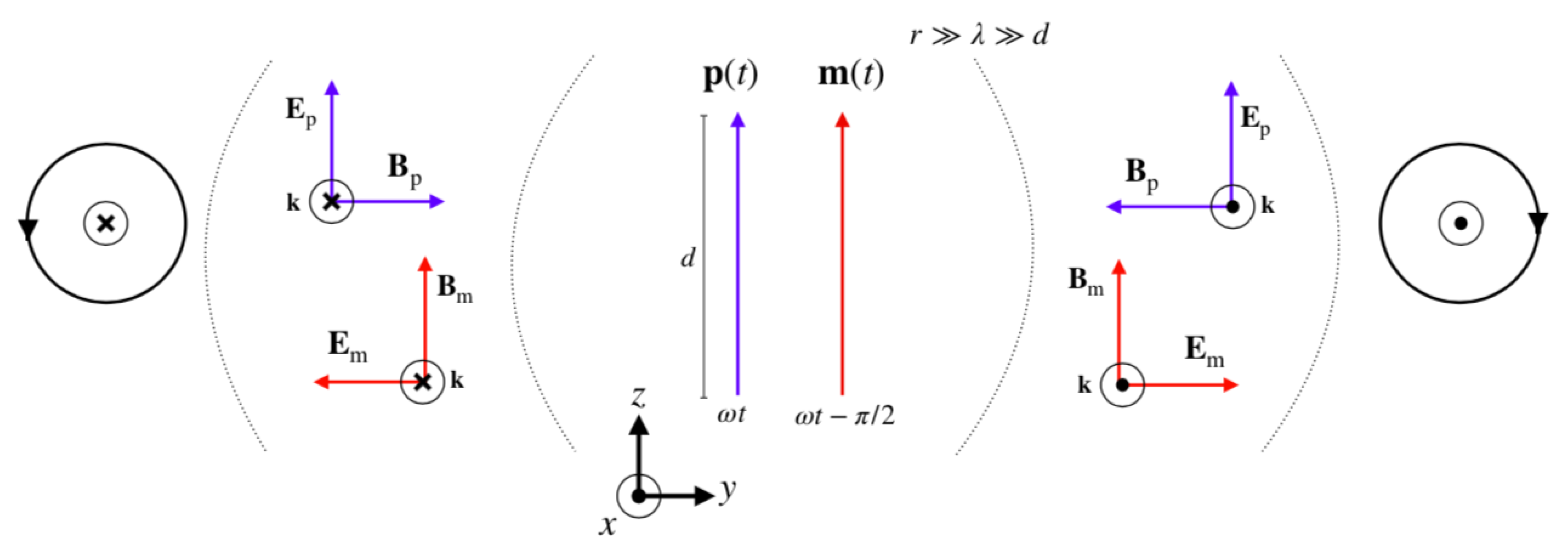
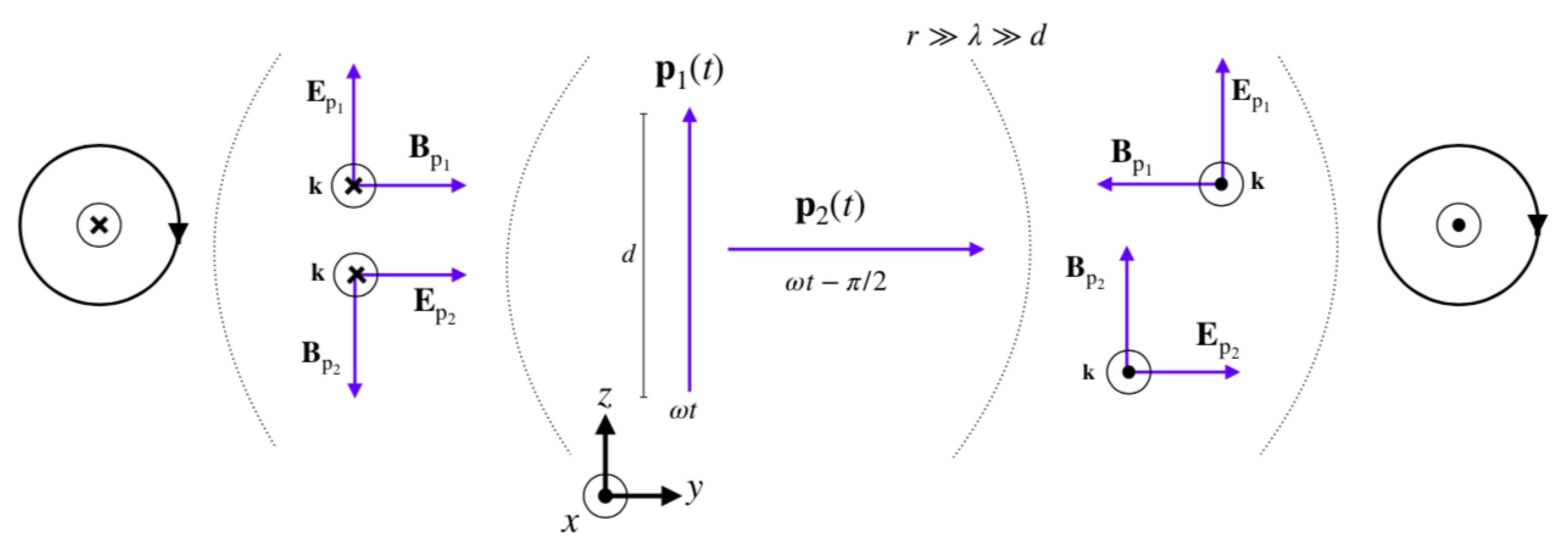
3.2. Dipole Model of a Helicity Source

As an illustration of how charges and currents can act as a source of helicity, we consider a point source consisting of an oscillating electric and a magnetic dipole, with electric and magnetic dipole moments $\mathbf{p}\left(t\right)$ and $\mathbf{m}\left(t\right)$, as has been examined by Leeder et al. [28]. This can be thought of as a simple model of a radiating chiral molecule, as the optical activity of chiral molecules ultimately arises from the simultaneous induction of electric and magnetic dipole moments through the electric-dipole magnetic-dipole polarisability tensor G [9] (see Chapter 3, §5.4). Leeder et al. treat the emission from the dipoles quantum-mechanically, calculating a differential irradiance for left- and right-circularly polarised light by considering the difference in decay rates into the two circular polarisation modes. From this, they obtain an expression for the net emitted helicity. There are three contributions to the total irradiance: one depending on ${\left|\mathbf{p}\right|}^2$, one on ${\left|\mathbf{m}\right|}^2$ and one on $\mathbf{p}·\mathbf{m}$. The mixed dipole term $\mathbf{p}·\mathbf{m}$ is the only contribution to the total irradiance that is different for the two enantiomers, and hence contributes to the net emitted helicity. We present here an analysis of helicity emission from the dipole system in the context of the continuity Equation (16), working within classical electromagnetism.

Consider an electric dipole oscillating along the $+z$ axis with dipole moment:

$$\begin{array}{c}\hfill \mathbf{p}\left(t\right)=p_{0}exp\left[i(\omega t+{\varphi }_{\mathrm{p}})\right]\widehat{\mathbf{z}},\end{array}$$

(18)

where we have defined $p_0=q_{0}d$, with d and $q_0$ the size and charge of the dipole, respectively. The resultant (retarded) vector potential in the far field defined by $d\ll \lambda \ll r$ is [43]:

$$\begin{array}{cc}\hfill {\mathbf{A}}_{\mathrm{p}}^{\prime }& =\Re \left[\frac{i\omega {\mu }_0{p}_0}{4\pi r}exp\left[i(\omega (t-r/c)+{\varphi }_{\mathrm{p}})\right]\widehat{\mathbf{z}}\right].\hfill \end{array}$$

(19)

We call this ${\mathbf{A}}_{\mathrm{p}}^{\prime }$, as we reserve the symbol $\mathbf{A}$ for the transverse part of the vector potential. From this expression, ${\mathbf{B}}_p$, ${\mathbf{E}}_{\mathrm{p}}$, ${\mathbf{C}}_{\mathrm{p}}$ and ${\mathbf{A}}_{\mathrm{p}}\equiv {\mathbf{A}}_{\mathrm{p}}^{{}^{\prime }\mathrm{T}}$ can be found.

Similarly, we consider a current oscillating in a loop of radius b in the $xy$ plane, $I\left(t\right)=I_{0}exp\left[i(\omega t+{\varphi }_{\mathrm{m}})\right]$. The resultant oscillating dipole moment is given by:

$$\begin{array}{cc}\hfill \mathbf{m}(t)=\int I(t)d\mathbf{a}& =m_{0}exp\left[i(\omega t+{\varphi }_{\mathrm{m}})\right]\widehat{\mathbf{z}},\hfill \end{array}$$

(20)

where $m_0=\pi b^2{I}_0$. The vector potential is calculated as [43]:

$$\begin{array}{cc}\hfill {\mathbf{A}}_{\mathrm{m}}& ={\mathbf{A}}_{\mathrm{m}}^{\mathrm{T}}=\Re \left[\frac{i\omega {\mu }_0{m}_0}{4\pi r^{2}c}\left(x\widehat{\mathbf{y}}-y\widehat{\mathbf{x}}\right)\right].\hfill \end{array}$$

(21)

Using this to find ${\mathbf{B}}_{\mathrm{m}}$, ${\mathbf{E}}_{\mathrm{m}}$ and ${\mathbf{C}}_{\mathrm{m}}$, we calculate the total helicity density and flux density of the combined electric-magnetic dipole system in the far-field:

$$\begin{array}{c}\hfill h_{\mathrm{pm}}=\frac{{ϵ}_0}{c}\left(\frac{{\mu }_0^2{m}_0{p}_0{\omega }^3}{16{\pi }^2{r}^4}\left(x^2+y^2\right)sin({\varphi }_{\mathrm{m}}-{\varphi }_{\mathrm{p}})\right),\end{array}$$

(22)

$$\begin{array}{c}\hfill {\mathbf{v}}_{\mathrm{pm}}={ϵ}_0\left(\frac{{\mu }_0^2{m}_0{p}_0{\omega }^3}{16{\pi }^2{r}^5}\left(x^2+y^2\right)sin({\varphi }_{\mathrm{m}}-{\varphi }_{\mathrm{p}})\right)\mathbf{r}.\end{array}$$

(23)

From (22), ${\partial }_t{h}_{\mathrm{pm}}=0$, and we use Gauss’s theorem to calculate the net helicity flux of the combined dipole system:

$$\begin{array}{c}\hfill \int \nabla ·{\mathbf{v}}_{\mathrm{pm}}{d}^3\mathbf{r}=\frac{{ϵ}_0{\mu }_0^2{m}_0{p}_0{\omega }^3}{6\pi }sin\left({\varphi }_{\mathrm{m}}-{\varphi }_{\mathrm{p}}\right).\end{array}$$

(24)

We can identify this with the source term on the right-hand side of (16). Noting $\int \mathbf{g}·(\nabla \times \mathbf{C})d^3\mathbf{r}=\int \mathbf{C}·(\nabla \times \mathbf{g})d^3\mathbf{r}$ [17], we obtain:

$$\begin{array}{c}\hfill \int \mathbf{g}·(\nabla \times \mathbf{C})d^3\mathbf{r}=\frac{{ϵ}_0{\mu }_0{m}_0{p}_0{\omega }^3}{6\pi c}sin\left({\varphi }_{\mathrm{m}}-{\varphi }_{\mathrm{p}}\right),\end{array}$$

(25)

which is maximised for a phase difference of $\pm \pi /2$ between the dipoles.

Left- and right-circularly polarised light can also be produced by a pair of orthogonally-aligned oscillating electric or magnetic dipoles. We consider the former configuration: ${\mathbf{p}}_1\left(t\right)=\left|{\mathbf{p}}_1\left(t\right)\right|\widehat{\mathbf{z}}$ and ${\mathbf{p}}_2\left(t\right)=\left|{\mathbf{p}}_2\left(t\right)\right|\widehat{\mathbf{y}}$, with a phase difference of ${\varphi }_{{\mathrm{p}}_2}-{\varphi }_{{\mathrm{p}}_1}$ between the oscillations. The resultant helicity flux density in the far-field is:

$$\begin{array}{cc}\hfill {\mathbf{v}}_{\mathrm{pp}}& =\frac{{ϵ}_{0}c}{2}\left(\frac{{\mu }_0^2{p}_0^2{\omega }^3}{16{\pi }^2{r}^5}sin({\varphi }_{\mathrm{p}}2-{\varphi }_{\mathrm{p}}1)xr\right)\mathbf{r},\hfill \end{array}$$

(26)

again maximised for ${\varphi }_{\mathrm{p}}2-{\varphi }_{\mathrm{p}}1=\pi /2$. The helicity density of this coupled dipole system is again time independent, so that the “source term” is found in analogy with the above calculation. We find $\int \nabla ·{\mathbf{v}}_{\mathrm{pp}}{d}^3\mathbf{r}$=0: the coupled electric-electric dipole system does not describe a source of helicity.

These results follow intuitively by considering Figure 2 and Figure 3, where the far-field patterns of the electric-magnetic and electric-electric dipole systems in the $yz$ plane have been drawn. A $\pi /2$ phase difference between the dipole oscillations results in right-circular polarisation in the $+x$ direction in both dipole systems. In the $-x$ direction, however, we obtain left-circular polarisation for the electric-magnetic dipole pair and right-circular polarisation for the electric-electric dipoles. Thus, we obtain a net flux of helicity for the electric-magnetic dipole system only.

The results of this calculation are intimately related to the respective parity of the electric-magnetic and electric-electric dipole systems. Considering again Figure 2, a parity transformation reverses the direction of the electric dipole only, so that the field patterns in both the $+x$ and the $-x$ direction are reversed, and a net flux of left-circular polarisation is produced. A parity transformation $\widehat{\mathbf{P}}$ thus interconverts the two “enantiomeric” configurations of the electric-magnetic dipole systems and produces a negative sign in the integrated source term in (25). The two enantiomeric forms can therefore be described simply by the aligned and anti-aligned configurations (or equivalently, as a positive or negative phase difference between the two oscillations in either configuration), which can be distinguished in the far-field $yz$ plane by an excess of right- or left-circular polarisation, respectively.

For the electric-electric dipoles in Figure 3, however, both dipoles are reversed under $\widehat{\mathbf{P}}$, so that the field patterns in $\pm x$ directions remain unchanged. As the electric-electric system is parity-even, but left- and right-circularly polarised fields are reversed under a parity transformation, it follows that the electric-electric dipole system cannot produce an excess of either polarisation and hence cannot be used to describe a source of helicity.

4. Macroscopic Sources

4.1. Helicity in Achiral, Reciprocal Media

We have seen how helicity can be produced by a microscopic source (a dipole), but it is also possible to discuss the generation of helicity within the framework of macroscopic electromagnetism in dielectric media. It is perhaps surprising that even in the presence of matter, there are some situations in which the helicity of an arbitrary electromagnetic field is still conserved. The conditions under which the electromagnetic helicity is conserved within media have been studied in recent years [16,18,19]. Fernandez-Corbaton et al. [16] consider the propagation of helicity in isotropic, lossless linear media, and these results are extended by van Kruining and Götte in [18] to include anisotropic and general linear media. Alpeggiani et al. [19] further consider helicity in a dispersive, lossy medium, while the electromagnetic chirality is examined in such media by Vázquez-Lozano and Martínez [44].

In the following, we consider a linear, lossless and isotropic medium. If the medium is comprised of distinct, homogeneous regions labelled by i, helicity is conserved so long as ${ϵ}_i/{\mu }_i$ remains constant for all i [16]. Following a similar method to that used in Section 2.5, we can derive a continuity equation for helicity in such media. We use the definitions of h (1) and $\mathbf{v}$ (14), along with the constitutive relations $\mathbf{D}=ϵ\mathbf{E}$ and $\mathbf{B}=\mu \mathbf{H}$, to obtain:

$${\partial }_{t}h+\nabla ·\mathbf{v}=\frac{1}{2}\left[\nabla \left(\sqrt{\frac{ϵ}{\mu }}\right)·\left(\mathbf{E}\times \mathbf{A}\right)+\nabla \left(\sqrt{\frac{\mu }{ϵ}}\right)·\left(\mathbf{H}\times \mathbf{C}\right)\right],$$

(27)

where we have allowed for the possibility that $ϵ$ and $\mu$ are functions of position. This explicitly shows the conservation of helicity when $\nabla \left(ϵ/\mu \right)=0$, which can be seen as a continuous statement of the result for stratified media presented in [16].

We extend the results of [17] discussed in Section 3.1, to examine the effects of inserting a local current density $\mathbf{j}$ into a medium described by the constitutive relations $\mathbf{D}=ϵ\mathbf{E}$ and $\mathbf{B}=\mu \mathbf{H}$. We find a source term analogous to the right-hand side of (16), but with the replacement of ${ϵ}_0\to ϵ$ and ${\mu }_0\to \mu$. Moreover, this type of source cannot be associated with that produced by a gradient of $ϵ/\mu$, as given by the right-hand side of (27).

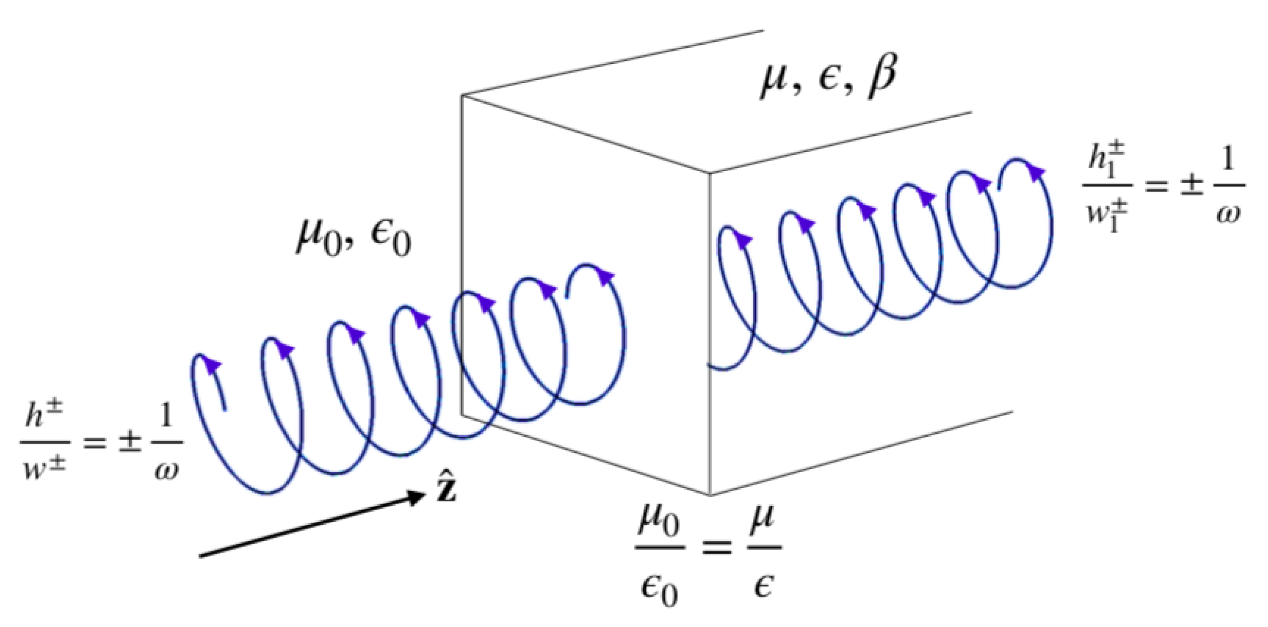
4.2. Helicity in Bi-Isotropic Media

We model a general linear, lossless bi-isotropic medium, where we allow for both a chiral and a magnetoelectric response, using an extension of the “Drude–Born–Fedorov” constitutive relations to include the Tellegen parameter $\alpha$ [45]:

$$\begin{array}{cc}\mathbf{D}& =ϵ\left(\mathbf{E}+\beta \nabla \times \mathbf{E}\right)+\alpha \mathbf{H},\\ \mathbf{B}& =\mu \left(\mathbf{H}+\beta \nabla \times \mathbf{H}\right)+\alpha \mathbf{E},\end{array}$$

(28)

where $\beta$ is the referred to as the chirality parameter. The results of [16] have been extended to include chiral and Tellegen media, as well an anisotropic polarisabilities, in [18], where it has been explicitly shown that Maxwell’s equations in a medium remain invariant under a duality transformation of the fields when there is a constant ratio $ϵ/\mu$ and a Tellegen parameter of zero. The chirality parameter, on the other hand, is free to vary in space. This result in [18] is based on the symmetrized constitutive relations of Condon [45], but it is straightforward to show that the same condition for dual symmetry holds for the Drude–Born–Fedorov relations given above.

Inserting the constitutive relations (28) with $\alpha =0$ into the helicity density and flux density (1) and (14) reveals that the conservation of helicity in a chiral medium cannot be expressed by a local continuity equation unless the expression for the helicity density inside a chiral medium is suitably modified [46].

Helicity Conservation in a Chiral Medium

Both helicity and energy are conserved in a lossless chiral medium [18,47]. It therefore follows that, in a situation where the interface between the vacuum and the medium is dual-symmetric, the helicity per photon of light in the chiral medium should remain the same as the vacuum values. This is the situation depicted in Figure 4. In [14], free electromagnetic fields with left- and right-circular polarisation are shown to have a helicity of $\pm \hslash$ per photon. In [46], the expressions for the helicity density and flux density (1) and (14) are trivially extended to those in a linear medium by replacement of the vacuum electric and magnetic responses, ${ϵ}_0$ and ${\mu }_0$, with $ϵ$ and $\mu$. In considering the propagation of left- and right-circularly polarised light within a chiral medium, is it shown that, although the flux density formed in this way produces the correct helicity of $\pm \hslash$ per photon, the helicity density does not. This follows from the fact that the energy density within a chiral medium is of the form [48]:

$$\begin{array}{c}\hfill w_1=\frac{1}{2}\left[\mathbf{D}·\mathbf{E}+\mathbf{B}·\mathbf{H}-\beta ϵ\mu (\mathbf{E}·\dot{\mathbf{H}}-\dot{\mathbf{E}}·\mathbf{H})\right],\end{array}$$

(29)

containing an explicit $\beta$-dependent term. As we know the correct form of the helicity flux density within the medium is:

$$\begin{array}{c}\hfill \mathbf{v}=\frac{1}{2}\left(\sqrt{\frac{ϵ}{\mu }}\mathbf{E}\times \mathbf{A}+\sqrt{\frac{\mu }{ϵ}}\mathbf{H}\times \mathbf{C}\right),\end{array}$$

(30)

we can use this and the condition of local helicity conservation to find the form of the helicity density. We find:

$$\begin{array}{ll}\nabla ·\mathbf{v}& =\frac{1}{2}\left(\sqrt{\frac{ϵ}{\mu }}\left(\mathbf{A}·(\nabla \times \mathbf{E})-\mathbf{E}·(\nabla \times \mathbf{A})\right)-\sqrt{\frac{\mu }{ϵ}}\left(\mathbf{C}·(\nabla \times \mathbf{H})-\mathbf{H}·(\nabla \times \mathbf{C})\right)\right)\\ & =\frac{1}{2}\left(\sqrt{\frac{ϵ}{\mu }}\left(-\mathbf{A}·\dot{\mathbf{B}}-\mathbf{E}·\mathbf{B}\right)-\sqrt{\frac{\mu }{ϵ}}\left(\mathbf{C}·\dot{\mathbf{D}}+\mathbf{H}·\mathbf{D}\right)\right),\end{array}$$

(31)

and use the product rule to write this as:

$$\begin{array}{c}\hfill \nabla ·\mathbf{v}=-{\partial }_t\frac{1}{2}\left(\sqrt{\frac{ϵ}{\mu }}\mathbf{A}·\mathbf{B}-\sqrt{\frac{\mu }{ϵ}}\mathbf{C}·\mathbf{D}\right)-\left(\sqrt{\frac{ϵ}{\mu }}\mathbf{E}·\mathbf{B}-\sqrt{\frac{\mu }{ϵ}}\mathbf{H}·\mathbf{D}\right).\end{array}$$

(32)

Identifying the time derivative as ${\partial }_{t}h$ and inserting the constitutive relations (28) with $\alpha =0$ leads to:

$$\begin{array}{cc}\hfill \nabla ·\mathbf{v}& =-{\partial }_{t}h-\sqrt{ϵ\mu }\beta \left[\mathbf{E}·\dot{\mathbf{D}}+\mathbf{H}·\dot{\mathbf{B}}\right],\hfill \end{array}$$

(33)

which is rearranged to produce:

$$\begin{array}{c}\hfill {\partial }_t\left(h+\sqrt{ϵ\mu }\beta w\right)+\nabla ·\mathbf{v}=0,\end{array}$$

(34)

where $w=1/2\left(\mathbf{D}·\mathbf{E}+\mathbf{B}·\mathbf{H}\right)$ is the energy density in an achiral medium. Equation (34) is correct to first order in the chirality parameter, denoted $\mathcal{O}\left(\beta \right)$, by which we mean that we neglect terms multiplied by ${\beta }^2$, or higher powers. This is incorporated into the definition of the helicity density h to form [46]:

$$\begin{array}{c}\hfill h_1=\frac{1}{2}\left(\sqrt{\frac{ϵ}{\mu }}\mathbf{A}·\mathbf{B}-\sqrt{\frac{\mu }{ϵ}}\mathbf{C}·\mathbf{D}\right)+\sqrt{ϵ\mu }\beta w.\end{array}$$

(35)

It is further shown in [46] that this indeed produces a helicity to energy density ratio of $\pm 1/\omega$ for right- and left-circularly polarised light, leading to a helicity of $\pm \hslash$ per photon [47]. In addition, it can be shown that higher order terms in $\beta$ of the helicity and energy densities retain this correspondence between the definitions, i.e.:

$$\begin{array}{c}\hfill h_{n+1}=\frac{1}{2}\left(\sqrt{\frac{ϵ}{\mu }}\mathbf{A}·\mathbf{B}-\sqrt{\frac{\mu }{ϵ}}\mathbf{C}·\mathbf{D}\right)+\sqrt{ϵ\mu }\beta w_n,\end{array}$$

(36)

such that ${\partial }_t{w}_n+\nabla ·\mathbf{S}=0$ and ${\partial }_t{h}_{n+1}+\nabla ·\mathbf{v}=0$, where $w_n$ is the energy density of the fields to $\mathcal{O}\left({\beta }^n\right)$ and $\mathbf{S}=\mathbf{E}\times \mathbf{H}$ is the energy flux density. This follows from the exact expression:

$$\begin{array}{c}\hfill {\partial }_{t}h+\nabla ·\mathbf{v}=\sqrt{ϵ\mu }\beta \nabla ·\mathbf{S},\end{array}$$

(37)

such that energy conservation to all orders in $\beta$ implies helicity conservation to all orders in $\beta$.

We can examine the general form of a source of helicity in lossless non-reciprocal media by inserting the constitutive relations (28) with $\alpha \ne 0$ into $h_1$ and $\mathbf{v}$, producing:

$$\begin{array}{cc}\hfill {\partial }_t{h}_1+\nabla ·\mathbf{v}& =-\alpha \left(\sqrt{\frac{ϵ}{\mu }}{\left|\mathbf{E}\right|}^2-\sqrt{\frac{\mu }{ϵ}}{\left|\mathbf{H}\right|}^2\right),\hfill \end{array}$$

(38)

where we have imposed $\nabla (ϵ/\mu )=0$. As the energy is conserved [47], it follows that the helicity per photon of the light within a Tellegen material must differ from the familiar free-space values.

4.3. Currents and Charges in Bi-Isotropic Media

We now consider what happens when a local current density is placed inside a chiral medium. Inserting the constitutive relations (28) into $\nabla \times \mathbf{E}=-\dot{\mathbf{B}}$ and $\nabla \times \mathbf{H}=\dot{\mathbf{D}}+\mathbf{j}$ leads to:

$$\begin{array}{cc}\hfill \dot{\mathbf{A}}& =\beta \left(\nabla \times \mathbf{E}\right)+\frac{1}{ϵ}\left(\nabla \times \mathbf{C}+\alpha \mathbf{H}\right)\hfill \end{array}$$

(39)

and:

$$\begin{array}{c}\hfill \dot{\mathbf{C}}=\mathbf{g}+\beta \left(\nabla \times \mathbf{H}\right)-\frac{1}{\mu }\left(\nabla \times \mathbf{A}-\alpha \mathbf{E}\right),\end{array}$$

(40)

where again, $\nabla \times \mathbf{g}$ is equal to the transverse part of the current density. We insert $\dot{\mathbf{A}}$ and $\dot{\mathbf{C}}$ into ${\partial }_t{h}_1$ from (35) and find to $\mathcal{O}\left(\beta \right)$:

$$\begin{array}{cc}\hfill {\partial }_t{h}_1+\nabla ·\mathbf{v}& =\frac{1}{2}\sqrt{\frac{\mu }{ϵ}}\left[\mathbf{g}·\left(\nabla \times \mathbf{C}\right)+\mathbf{C}·\left(\nabla \times \mathbf{g}\right)\right]-\sqrt{ϵ\mu }\beta \mathbf{j}·\mathbf{E}-\alpha \left(\sqrt{\frac{ϵ}{\mu }}{\left|\mathbf{E}\right|}^2-\sqrt{\frac{\mu }{ϵ}}{\left|\mathbf{H}\right|}^2\right).\hfill \end{array}$$

(41)

This reduces to the result for a medium with no chiroptical or magnetoelectric response when $\alpha =\beta =0$. The helicity contribution due to the chiral response of the material is identifiable as an energy source, as obtained from the energy continuity equation in the presence of charges [41]. As this term is a scalar, the pseudoscalar nature of $\beta$ is responsible for this term’s acting as a source of helicity. The Tellegen contribution, proportional to $\alpha$, is identical to the helicity source in an absence of currents or charges, as given in (38).

Consider a chiral, reciprocal material described by (28) with $\alpha =0$. From (41), we would expect that an emitter that in free space emits no net helicity, such as a single oscillating electric dipole, may act as a source of helicity when placed inside a chiral medium. Lathakia et al. have shown that this is so, by explicitly calculating the radiation pattern of a single oscillating electric dipole embedded in a sphere composed of a lossless chiral medium [49]. From the point of view of an observer in the far field, outside the sphere, the radiation pattern from the point electric dipole embedded in the sphere appears identical to that of a point electric and point magnetic dipole oscillating in a vacuum. In particular, the chiral medium is impedance matched with the surrounding vacuum to produce this result, so that the net helicity cannot be attributed to a gradient in $ϵ/\mu$ at the vacuum-chiral interface. As the chiral medium considered above and in [49] is lossless, neither can this generation of helicity arise as a result of circular dichroism within the chiral sphere [30]. Furthermore, we know that the electromagnetic helicity of a field is conserved within a dual-symmetric chiral medium, so the helicity “source” in this case can only be attributed to the interaction of the embedded current and the chiral medium itself; a result which seems worthy of further investigation.

It is interesting to observe that for $\mathcal{O}\left(\beta \right)$, we can write $-\beta \mathbf{j}·\mathbf{E}=\beta \left(\nabla \times \mathbf{g}\right)·\left(\nabla \times \mathbf{C}\right)$, so that the current helicity source in the chiral medium appears as an even-parity combination of $\mathbf{g}$ and $\mathbf{C}$. We would expect terms $\mathcal{O}\left({\beta }^{2n+1}\right)$ to echo this structure, with even-order terms $\mathcal{O}\left({\beta }^{2n}\right)$ containing odd-parity combinations of $\mathbf{g}$ and $\mathbf{C}$, such as given by the first term on the right-hand side of (41).

5. Concluding Remarks

We have examined in detail the construction of the helicity density (1) in a vacuum and discussed the merits of using this quantity to characterise chiral light. Alongside this, we examined the chirality density (2) of the free electromagnetic field and pointed out cases in which the two quantities are trivially related. Only the conservation of helicity, however, generates a physically-meaningful symmetry transformation of the system. We used this to construct a continuity equation of the helicity of the free field, before extending the method to examine cases under which this symmetry is broken and helicity is no longer conserved. We have identified four distinct types of helicity sources. The first results from a non-constant value of $ϵ/\mu$, taking the form of the right-hand side of (27). The second helicity source has the general form of (16) [17] and can be understood in its simplest form in terms of a coupled electric-magnetic dipole system. The third results from the non-reciprocity parameter $\alpha$ in the constitutive relations, of the form (38). The final type of source examined in this article results from a dual-symmetric object embedded in a chiral medium, expressible as an energy source multiplied by the chirality parameter $\beta$, as given by (41).

Categorisation of the distinct sources of helicity in this way provides insight into the electromagnetic response of different types of matter and is achieved by exploiting the inherent symmetry of the Maxwell equations. The distinction between the microscopic and macroscopic sources results from the non-tractable nature of the problem of determining the electromagnetic response of large volumes (≫than the size of individual molecules) of helicity sources. In order to bridge this gap, we can perhaps look to experiments in which chiral objects are embedded into a dielectric host, forming an artificial composite chiral medium [50,51]. In recent work, such methods have been used to verify that a chiral nanostructure is in fact able to sense the orbital, as well as the spin angular momentum of an impinging light beam [52,53]. Theoretical study on this subject continues to reveal insight into the significance of twisted light beams in chiral light–matter interactions [54,55], paving the way for new methods in the detection and manipulation of chiral matter. The importance of helicity in the characterisation of both natural and engineered chiral nanostructures is indeed becoming increasingly apparent: Hanifeh et al. [56] show that using structured light with maximised helicity leads to a direct measure of the chirality of such an object, which does not require knowledge of the helicity or energy densities of the field. It is also evident that both the helicity of the incident fields and the dual-symmetry (or helicity preserving nature) of a photonic structure are essential in circular dichroism enhancement effects [57]. Reconciling our understanding of both microscopic and macroscopic sources of helicity in a general theoretical model, however, is an ongoing topic of investigation.

References

1. Arago, D. Sur une modification remarquable qu’éprouvent les rayons lumineux dans leur passage à travers certains corps diaphanes, et sur quelques autres nouveaux phénomènes d’optique. Mem. Inst. 1811, 1, 93–134. [Google Scholar]
2. Biot, J.B. Phénomènes de polarisation successive, observés dans les fluides homogènes. Bull. Soc. Philomath. 1815, 1, 190–192. [Google Scholar]
3. Pasteur, L. Recherches sur les relations qui peuvent exister entre la forme cristalline, la composition chimique et le sens de la polarisation rotatoire. Ann. Chim. Phys. 1848, 24, 442–459. [Google Scholar]
4. Van’T Hoff, J.H.; Pasteur, L.; Richardson, G.M.; Le Bel, J.A. The Foundations of Stereo Chemistry: Memoirs by Pasteur, Van’T Hoff, Lebel and Wilslincenus; American Book Company: Woodstock, GA, USA, 1901. [Google Scholar]
5. Kelvin, L. The Molecular Tactics of a Crystal; Clarendon Press: Oxford, UK, 1894. [Google Scholar]
6. Cameron, R.P.; Götte, J.B.; Barnett, S.M.; Yao, A.M. Chirality and the angular momentum of light. Philos. Trans. R. Soc. A Math. Phys. Eng. Sci. 2017, 375, 20150433. [Google Scholar] [CrossRef] [PubMed] [Green Version]
7. Lee, T.D.; Yang, C.N. Question of parity conservation in weak interactions. Phys. Rev. 1956, 104, 254–258. [Google Scholar] [CrossRef]
8. Wagnière, G.H. On Chirality and the Universal Asymmetry: Reflections on Image and Mirror Image; John Wiley and Sons: Hoboken, NJ, USA, 2007. [Google Scholar]
9. Barron, L.D. Molecular Light Scattering and Optical Activity; Cambridge University Press: Cambridge, UK, 2004. [Google Scholar]
10. Cotton, A. Absorption inégale des rayons circulaires droit et gauche dans certains corps actifs. Compt. Rend. 1895, 120, 989–991. [Google Scholar]
11. Poynting, J.H. The Wave Motion of a Revolving Shaft, and a Suggestion as to the Angular Momentum in a Beam of Circularly Polarised Light. Proc. R. Soc. A Math. Phys. Eng. Sci. 1909, 82, 560–567. [Google Scholar] [CrossRef] [Green Version]
12. Calkin, M.G. An Invariance Property of the Free Electromagnetic Field. Am. J. Phys. 1965, 33, 958–960. [Google Scholar] [CrossRef]
13. Trueba, J.L.; Rañada, A.F. The electromagnetic helicity. Eur. J. Phys. 1996, 17, 141–144. [Google Scholar] [CrossRef]
14. Barnett, S.M.; Cameron, R.P.; Yao, A.M. Duplex symmetry and its relation to the conservation of optical helicity. Phys. Rev. A 2012, 86, 013845. [Google Scholar] [CrossRef]
15. Cameron, R.P.; Barnett, S.M.; Yao, A.M. Optical helicity, optical spin and related quantities in electromagnetic theory. New J. Phys. 2012, 14, 053050. [Google Scholar] [CrossRef] [Green Version]
16. Fernandez-Corbaton, I.; Zambrana-Puyalto, X.; Tischler, N.; Vidal, X.; Juan, M.L.; Molina-Terriza, G. Electromagnetic duality symmetry and helicity conservation for the macroscopic maxwell’s equations. Phys. Rev. Lett. 2013, 111, 060401. [Google Scholar] [CrossRef] [PubMed]
17. Nienhuis, G. Conservation laws and symmetry transformations of the electromagnetic field with sources. Phys. Rev. A 2016, 93, 023840. [Google Scholar] [CrossRef]
18. van Kruining, K.; Götte, J.B. The conditions for the preservation of duality symmetry in a linear medium. J. Opt. 2016, 18, 085601. [Google Scholar] [CrossRef] [Green Version]
19. Alpeggiani, F.; Bliokh, K.Y.; Nori, F.; Kuipers, L. Electromagnetic Helicity in Complex Media. Phys. Rev. Lett. 2018, 120, 243605. [Google Scholar] [CrossRef] [PubMed] [Green Version]
20. Saffman, P.G. Vortex Dynamics; Cambridge University Press: New York, NY, USA, 1992. [Google Scholar]
21. Madja, A.J.; Bertozzi, A.L. Vorticity and Incompressible Flow; Cambridge University Press: Cambridge, UK, 2002. [Google Scholar]
22. Moffatt, H.K. The degree of knottedness of tangled vortex lines. J. Fluid Mech. 1969, 35, 117–129. [Google Scholar] [CrossRef]
23. Woltjer, L. A theorem on force-free magnetic fields. Proc. Natl. Acad. Sci. USA 1958, 44, 489–491. [Google Scholar] [CrossRef] [PubMed]
24. Priest, E.; Forbes, T. Magnetic Reconnection: MHD Theory and Applications; Cambridge University Press: New York, NY, USA, 2000. [Google Scholar]
25. Cameron, R.P. On the ‘second potential’ in electrodynamics. J. Opt. 2014, 16, 015708. [Google Scholar] [CrossRef]
26. Fernandez-Corbaton, I.; Vidal, X.; Tischler, N.; Molina-Terriza, G. Necessary symmetry conditions for the rotation of light. J. Chem. Phys. 2013, 138, 214311. [Google Scholar] [CrossRef] [PubMed] [Green Version]
27. Coles, M.M.; Andrews, D.L. Chirality and angular momentum in optical radiation. Phys. Rev. A 2012, 85, 63810. [Google Scholar] [CrossRef]
28. Leeder, J.M.; Haniewicz, H.T.; Andrews, D.L. Point source generation of chiral fields: Measures of near-and far-field optical helicity. J. Opt. Soc. Am. B 2015, 32, 2308–2313. [Google Scholar] [CrossRef]
29. Lipkin, D.M. Existence of a new conservation law in electromagnetic theory. J. Math. Phys. 1964, 5, 696–700. [Google Scholar] [CrossRef]
30. Tang, Y.; Cohen, A.E. Optical Chirality and Its Interaction with Matter. Phys. Rev. Lett. 2010, 104, 163901. [Google Scholar] [CrossRef] [PubMed]
31. Tang, Y.; Cohen, A.E. Enhanced Enantioselectivity in Excitation of Chiral Molecules by Superchiral Light. Science 2011, 332, 333–336. [Google Scholar] [CrossRef] [PubMed]
32. Abdulrahman, N.; Syme, C.D.; Jack, C.; Karimullah, A.; Barron, L.D.; Gadegaard, N.; Kadodwala, M. The origin of off-resonance non-linear optical activity of a gold chiral nanomaterial. Nanoscale 2013, 5, 12651–12657. [Google Scholar] [CrossRef] [PubMed] [Green Version]
33. Andrews, D.L.; Coles, M.M. Optical superchirality and electromagnetic angular momentum. In Complex Light and Optical Forces VI; International Society for Optics and Photonics: Bellingham, WA, USA, 2012; Volume 8274, pp. 827405–827407. [Google Scholar]
34. van Kruining, K.C.; Cameron, R.P.; Götte, J.B. Superpositions of up to six plane waves without electric-field interference. Optica 2018, 5, 1091–1098. [Google Scholar] [CrossRef]
35. Karczmarek, J.; Wright, J.; Corkum, P.; Ivanov, M. Optical centrifuge for molecules. Phys. Rev. Lett. 1999, 82, 3420–3423. [Google Scholar] [CrossRef]
36. Van Enk, S.J.; Nienhuis, G. Spin and Orbital Angular Momentum of Photons. Europhys. Lett. 1994, 25, 497–501. [Google Scholar] [CrossRef]
37. van Enk, S.J.; Nienhuis, G. Commutation rules and eigenvalues of spin and orbital angular momentum of radiation fields. J. Mod. Opt. 1994, 41, 963–977. [Google Scholar] [CrossRef]
38. Barnett, S.M. Rotation of electromagnetic fields and the nature of optical angular momentum. J. Mod. Opt. 2010, 57, 1339–1343. [Google Scholar] [CrossRef] [PubMed] [Green Version]
39. Barnett, S.M.; Allen, L.; Cameron, R.P.; Gilson, C.R.; Padgett, M.J.; Speirits, F.C.; Yao, A.M. On the natures of the spin and orbital parts of optical angular momentum. J. Opt. 2016, 18, 064004. [Google Scholar] [CrossRef]
40. Cameron, R.P.; Speirits, F.C.; Gilson, C.R.; Allen, L.; Barnett, S.M. The azimuthal component of Poynting’s vector and the angular momentum of light. J. Opt. 2015, 17, 125610–125618. [Google Scholar] [CrossRef]
41. Jackson, J.D. Classical Electrodynamics, 3rd ed.; Wiley: New York, NY, USA, 1962. [Google Scholar]
42. Berry, M.V. Optical currents. J. Opt. A Pure Appl. Opt. 2009, 11, 094001. [Google Scholar] [CrossRef]
43. Griffiths, D.J. Introduction to Electrodynamics, 3rd ed.; Prentice Hall: Upper Saddle River, NJ, USA, 1999. [Google Scholar]
44. Vázquez-Lozano, J.E.; Martínez, A. Optical Chirality in Dispersive and Lossy Media. Phys. Rev. Lett. 2018, 121, 043901. [Google Scholar] [CrossRef] [PubMed]
45. Lakhtakia, A. Beltrami Fields in Chiral Media; World Scientific Series in Contemporary Chemical Physics; World Scientific: Singapore, 1994. [Google Scholar]
46. Crimin, F.; Mackinnon, N.; Götte, J.B.; Barnett, S.M. On the helicity density in a chiral medium. 2019; in press. [Google Scholar]
47. Barnett, S.M.; Cameron, R.P. Energy conservation and the constitutive relations in chiral and non-reciprocal media. J. Opt. 2016, 18, 015404. [Google Scholar] [CrossRef]
48. Bursian, V.; Timorew, F.A. Zur Theorie der optisch aktiven isotropen Medien. Z. Phys. 1926, 38, 475–484. [Google Scholar] [CrossRef]
49. Lakhtakia, A.; Varadan, V.K.; Varadan, V.V. Radiation by a point electric dipole embedded in a chiral sphere. J. Phys. D App. Phys. 1990, 23, 481–485. [Google Scholar] [CrossRef]
50. Elezzabi, A.Y.; Sederberg, S. Optical activity in an artificial chiral media: A terahertz time-domain investigation of Karl F Lindman’s 1920 pioneering experiment. Opt. Express 2009, 17, 6600–6612. [Google Scholar] [CrossRef] [PubMed]
51. Wang, Z.; Cheng, F.; Winsor, T.; Liu, Y. Optical chiral metamaterials: A review of the fundamentals, fabrication methods and applications. Nanotechnology 2016, 27, 412001–412021. [Google Scholar] [CrossRef] [PubMed]
52. Brullot, W.; Vanbel, M.K.; Swusten, T.; Verbiest, T. Resolving enantiomers using the optical angular momentum of twisted light. Sci. Adv. 2016, 2, e1501349. [Google Scholar] [CrossRef] [PubMed] [Green Version]
53. Woźniak, P.; De León, I.; Höflich, K.; Leuchs, G.; Banzer, P. Interaction of light carrying orbital angular momentum with a chiral dipolar scatterer. arXiv, 2019; arXiv:1902.01731. [Google Scholar]
54. Forbes, K.A.; Andrews, D.L. Optical orbital angular momentum: Twisted light and chirality. Opt. Lett. 2018, 43, 435–438. [Google Scholar] [CrossRef] [PubMed]
55. Forbes, K.A.; Andrews, D.L. The angular momentum of twisted light in anisotropic media: Chiroptical interactions in chiral and achiral materials. In Nanophotonics VII; International Society for Optics and Photonics: Bellingham, WA, USA, 2018; Volume 10672. [Google Scholar]
56. Hanifeh, M.; Albooyeh, M.; Capolino, F. Optimally Chiral Electromagnetic Fields: Helicity Density and Interaction of Structured Light with Nanoscale Matter. arXiv, 2018; arXiv:1809.04117. [Google Scholar]
57. Graf, F.; Feis, J.; Garcia-Santiago, X.; Wegener, M.; Rockstuhl, C.; Fernandez-Corbaton, I. Achiral, Helicity Preserving, and Resonant Structures for Enhanced Sensing of Chiral Molecules. ACS Photonics 2019. [Google Scholar] [CrossRef]
Figure 1. (a) The molecule bromochlorofluoromethane is chiral, as the molecule and its mirror image cannot be superimposed, even after rotation. (b) Dichlorofluoromethane, on the other hand, is achiral, as the molecule can be superimposed upon its mirror image after rotation.
Applsci 09 00828 g001
Figure 2. Oscillating electric p ( t ) and magnetic m ( t ) dipoles aligned along the z axis, with the latter lagging by a phase of π / 2 . The far-field pattern is that of right-circularly polarised light in the + x direction and left-circularly polarised light in the x direction: there is a net flux of right-circular polarisation in the y z plane.
Applsci 09 00828 g002
Figure 3. Two oscillating electric dipoles, labelled p 1 ( t ) and p 2 ( t ) , oscillate along the z and y axes, respectively, with a phase difference of π / 2 . The far-field pattern in the + x direction is identical to that produced by the electric-magnetic dipole configuration in Figure 2, but has opposite polarisation in the x direction: the net helicity flux in the y z plane is zero.
Applsci 09 00828 g003
Figure 4. At the interface between a vacuum and a dual-symmetric, lossless chiral medium characterised by ϵ , μ and the chirality parameter β , both the energy and helicity of an electromagnetic field are conserved. As a consequence, the ratio of the helicity density to energy density, h / w , must be preserved across the interface. In the chiral medium, the energy density contains a chiral contribution, as given by w 1 (29), requiring a modification of the helicity density to h 1 (35) such that h / w = h 1 / w 1 holds.
Applsci 09 00828 g004