A Grid-Based Swarm Intelligence Algorithm for Privacy-Preserving Data Mining

Abstract

Privacy-preserving data mining (PPDM) has become an interesting and emerging topic in recent years because it helps hide confidential information, while allowing useful knowledge to be discovered at the same time. Data sanitization is a common way to perturb a database, and thus sensitive or confidential information can be hidden. PPDM is not a trivial task and can be concerned an Non-deterministic Polynomial-time (NP)-hard problem. Many algorithms have been studied to derive optimal solutions using the evolutionary process, although most are based on straightforward or single-objective methods used to discover the candidate transactions/items for sanitization. In this paper, we present a multi-objective algorithm using a grid-based method (called GMPSO) to find optimal solutions as candidates for sanitization. The designed GMPSO uses two strategies for updating gbest and pbest during the evolutionary process. Moreover, the pre-large concept is adapted herein to speed up the evolutionary process, and thus multiple database scans during each evolutionary process can be reduced. From the designed GMPSO, multiple Pareto solutions rather than single-objective algorithms can be derived based on Pareto dominance. In addition, the side effects of the sanitization process can be significantly reduced. Experiments have shown that the designed GMPSO achieves better side effects than the previous single-objective algorithm and the NSGA-II-based approach, and the pre-large concept can also help with speeding up the computational cost compared to the NSGA-II-based algorithm.

1. Introduction

Data mining, also called knowledge discovery in databases [1,2,3,4,5,6], is used to find the useful and meaningful information for further decision-making, and can be utilized in many domains and applications, including basket analytics, DNA sequence analysis, or recommendations. During the mining process, although useful information is discovered, confidential/sensitive information is also revealed at the same time, which causes security and privacy threats. Privacy-preserving data mining (PPDM) [7,8,9,10] has thus become an important topic in recent decades because it can not only hide private information but also discover the required information through varied data mining techniques. Data sanitization is a way to hide sensitive information by perturbing the database, although this process can also bring about side effects such as a hiding failure, missing cost, or artificial cost. A hiding failure indicates confidential information that has been thought to be hidden but still remains after a sanitization process and can be discovered during the mining process. A missing cost indicates already discovered information that may be missed after the sanitization process, whereas an artificial cost indicates meaningless or unnecessary information that has not been discovered but is mined after the sanitization process. Such side effects can also be regarded as an Non-deterministic Polynomial-time (NP)-hard problem [7,10] because more confidential information is hidden, and greater loss or an increased amount of information can appear. Many algorithms have been developed to minimize these three side effects during the sanitization process, including straightforward (conventional) or optimization processes. Lindell and Pinkas presented an ID3 algorithm [11] to solve the problem of PPDM based on a decision-tree. Clifton et al. then presented a toolkit to solve the problem of a PPDM [12]. Dwork et al. [13] designed several algorithms for handling published noisy statistics to vertically partitioned databases. Wu et al. [14] then designed several algorithms to reduce the support/confidence for hiding sensitive information. Hong et al. [15] utilized the Term Frequency-Inverse Document Frequency (TF-IDF) method and presented the Sensitive Itemset Frequency-Inverse Document Frequency (SIF-IDF) algorithm to evaluate the score of each transaction for data sanitization. Several studies related to PPDM have been conducted, most of which are based on a deletion procedure to hide sensitive information [15,16,17,18].

Because the PPDM is a non-trivial and NP-hard problem, it is thus difficult to find optimized solutions between the side effects. Several algorithms based on the evolutionary computation have been designed to obtain the optimal solutions. For instance, Lin et al. utilized genetic algorithms (GAs) to sanitize a database and presented the cpGA2DT and pGA2DT algorithms [19,20]. A good performance has been shown in terms of side effects as compared to a greedy-based algorithm. Although the above algorithms can achieve a good performance in terms of side effects, they rely on the pre-defined weights of three side effects in their pre-defined fitness function. This problem causes the results of the side effects to be seriously influenced by the weighted values; the results are occasionally not optimized, which requires a priori knowledge or an expert to set up these weighted values. To handle this problem, Cheng et al. [21] developed the Evolutionary Multiobjective Optimization (EMO)-based algorithm to consider “data distortion” and “knowledge distortion” in the sanitization process through item deletion. Although this approach concerns multi-objective functions, it may lead to finding incomplete knowledge for decision-making because it directly deletes the attributes from the database, which is not applicable to a sequential dataset.

Non-dominated Sorting Genetic Algorithm (NSGA)-II [22] is a way to regard multi-objective functions rather than a single-objective function. Lin et al. [23] developed an algorithm by adapting the NSGA-II model for data sanitization in PPDM. The multi-objective particle swarm optimization (MOPSO) algorithm [24] was extended from a conventional particle swarm optimization (PSO) algorithm [25], but handles multi-objective problems to find a set of Pareto solutions. However, the MOPSO framework cannot be directly applied to handle the problem of PPDM because the dominance relationships should be utilized to obtain the optimized transactions for deletion. In this study, we utilize the MOPSO framework and present a grid-based algorithm called GMPSO. The major contributions of the study are summarized below.

• This is the first work regarding the design of an MOPSO-based framework in PPDM, which shows a better performance in terms of side effects compared to a conventional single-objective approach and the NSGA-II-based model.
• We present two updating strategies for the global best (gbest) and personal best (pbest) solutions during the updating process of the MOPSO framework, which can be utilized in the PPDM problem for obtaining un-dominated solutions.
• To speed up the evolutionary process, the pre-large concept is utilized here to speed up the process of the evaluated solution, and thus multiple database scans can be greatly avoided.
• Experiment results demonstrate the performance of the designed GMPSO in terms of the time cost and four side effects as compared to a traditional single-objective algorithm and the NSGA-II-based approach.

The rest of this paper is organized as follows. A literature review is provided in Section 2. Preliminary information and a problem statement are given in Section 3. The developed GMPSO with two updating strategies is described in Section 4. An illustrated example is provided in Section 5. Several experiments conducted on varied datasets are detailed in Section 6. Finally, some concluding remarks and areas of future study are discussed in Section 7.

2. Literature Review

The studies relevant to evolutionary computation, privacy-preserving data mining (PPDM), and pre-large concepts are described as follows.

2.1. Evolutionary Computation

Evolutionary computation was inspired by the idea of biological evolution, which is used to solve an NP-hard problem by providing the optimal solutions in different applications and domains. Holland applied Darwin’s theory of natural selection and survival of the fittest to develop genetic algorithms (GAs) [26,27], which are widely used in computational intelligence for solving the NP-hard problem. GAs consist of several operations, for instance, selection, crossover, and mutation, used to evaluate the solutions iteratively during the evolutionary process. Particle swarm optimization (PSO) is a swarm intelligence algorithm proposed by Kennedy and Eberhart. It was inspired by bird flocking activities [25] to search the optimal solutions, in which each particle in the PSO is regarded as a potential solution. In a PSO, each bird has its own velocity, which is used to represent the direction to the other solutions. Moreover, each particle is then updated with its own best value (represented as pbest) and global best value (represented as gbest) according to the designed fitness function during each iteration. The particle is then updated using gbest, pbest, and its own velocity during each iteration. These processes are listed as follows [25]:

$$v_i(t+1)=w\times v_i(t)+c_1\times r_1\times (pbes{t}_i-x_i(t))+c_2\times r_2\times (gbest-x_i(t)),$$

(1)

$$x_i(t+1)=x_i(t)+v_i(t+1).$$

(2)

From the above equations, w is considered a factor used to balance the influence of global and local searches, $v_i$ represents the velocity of the i-th particle in a population where t presents the t-th iteration. Here, $c_1$ and $c_2$ are constant values. Both $r_1$ and $r_2$ are random numbers generated through a uniform distribution within the range of [0, 1]. The velocity of the particle is updated by Equation (1), and its position is updated by Equation (2). Several meta-heuristic algorithms have been respectively presented and applied to several realistic problems and situations to search the optimal solutions, for instance, ant colony optimization [28] or an artificial bee colony [29].

The above algorithms mostly regard single-objective optimization in a fitness function, and thus the derived solutions cannot be optimized because, in real-world applications, we may regard more than two objectives together to obtain the solutions. Multi-objective genetic algorithms [30], a non-dominated sorting genetic algorithm (NSGA) [31], and the NSGA-II model [32] were respectively designed to regard more objectives for obtaining Pareto solutions. Each solution in the Pareto solution has a non-dominated relation to the others. Extensions of the multi-objective algorithms have been respectively studied, for example, the strength Pareto evolutionary algorithm [33] and Pareto archived evolution strategy [34]. Coello et al. introduced the multi-objective particle swarm optimization framework [24] that applies the adaptive grid method to maintain an external archive, change the direction of the particles to keep them from flying out of the search space, and keep the particles within the boundary. Several algorithms based on the evolutionary computations are extensively presented in different domains and applications [35,36,37].

2.2. Privacy-Preserving Data Mining

During the past two decades, data mining has been an efficient way to find potential and useful information from a very large database, particularly the relationships between those products that may not be easily discovered and visualized. Because information can be revealed from a database, confidential/secure information can also be discovered during the mining procedure, thereby causing privacy and security threats to users. Privacy-preserving data mining (PPDM) has become a critical issue in recent years because, not only can it find useful information, but confidential/secure data can also be hidden using a sanitization procedure; such confidential information can thus be hidden and not discovered after data sanitization. Agrawal and Srikant [38] developed a novel reconstruction approach that can accurately estimate the distribution of original data. The classifiers can also be constructed to compare the accuracy between the original and sanitized data. Verykios et al. [10] developed hierarchical classification techniques used in PPDM. Dasseni et al. [16] then designed an approach based on a Hamming-distance mechanism to decrease the support or confidence of sensitive information (i.e., association rules) for sanitization. Oliveira and Zaiane [9] provided several sanitization methods that can hide frequent itemsets through a heuristic framework. The developed algorithms use an item-restriction approach to avoid a noise addition and limit the removal of real datasets. Islam and Brankovic [39] presented a framework using the noise addition method to protect and hide individual privacy while still maintaining a high data quality. Hong et al. provided an SIF-IDF method [15] to assign a weight to each transaction, and a sanitization process is then conducted from the transaction with the highest score to that of the lowest score for sanitization purposes.

The PPDM is considered as an NP-hard problem [7,10], however; it is thus better to provide meta-heuristic approaches to find the optimal solutions. Han and Ng developed a secure protocol [40] to find a better set of rules without disclosing their own private data based on GAs [26,27], and the result of the true positive rate times the true negative rate is then calculated to evaluate each decision rule. Lin et al. then presented several GA-based approaches, including sGA2DT, pGA2DT [20], and cpGA2DT [19] to hide the sensitive information by removing the victim transactions. The encoded chromosome is considered a set of solutions, and the transaction of a gene within a chromosome is regarded as the victim for later deletion. A fitness function was also developed to consider three side effects for an evaluation with pre-defined weights to show the goodness of the chromosome. Although the above algorithms are efficient at finding the optimal transactions for deletion, they still require pre-defined weights of the side effects; such a mechanism can seriously affect the final results of the designed approaches. Cheng et al. [21] thus developed an Evolutionary Multiobjective Optimization-Rule Hiding (EMO-RH) algorithm to hide the sensitive itemsets by removing the itemsets based on the EMO. This approach is based on a multi-objective method, although incomplete transactions can therefore be produced; a misleading decision can thus occur, particularly in the treatment of hospital diagnoses. Lin et al. presented a meat-heuristic approach [23] based on the NSGA-II framework for data sanitization, which shows better side effects compared to single-objective algorithms, which is the state-of-the-art multiple-objective optimization algorithm in PPDM. Several works of privacy-preserving and security issues are extensively studied in different applications. For example, Hasan et al. [41] presented a new method for handling the privacy issue of independent published data. Liu and Li [42] mentioned a clustering-based method for anonymity problem in IoT devices.

2.3. Pre-Large Concept

The mining of useful and meaningful information is a critical target in data mining [1,2,43], and most of the studied algorithms have focused on mining information from a static database. Thus, when the size of the database changes, a conventional approach is to re-process the updated database and re-mine the required information again to reveal the most up-to-date information. The fast updated (FUP) concept [44] was presented to handle dynamic data mining, particularly for a transaction insertion. The FUP concept is efficient at updating discovered information, but it still needs to rescan the original database again in certain cases. The pre-large concept [45,46] was presented to more efficiently update the mined information, and can avoid the need for multiple database scans if the number of newly inserted transactions does not achieve the pre-defined safety bound. It uses two thresholds to maintain large (frequent) and pre-large itemsets, and treats pre-large itemsets as a buffer for later maintenance. Thus, movement of a large itemset directly to a small itemset can be significantly reduced, and vice versa. Although this approach needs extra memory use for a pre-large itemset, it is efficient at handling the problem of dynamic data mining, particularly for a transaction insertion. Figure 1 shows nine cases of the pre-large concept.

Figure 1 indicates that the itemsets in cases 2, 3, 4, 7, and 8 will not affect the final results of the frequent itemsets. In case 1, some frequent itemsets may be removed, and, in cases 5, 6, and 9, the newly frequent itemsets may be generated. If all large and pre-large itemsets are maintained, then cases 1, 5, and 6 can be easily handled. For a special case, such as case 9, an itemset cannot be a large itemset in the updated database if its support value satisfies the following equation:

$$f\le \frac{(S_u-S_l)\times \left|D\right|}{S_u},$$

(3)

where $S_u$ is the upper-bound value, which is the same as the traditional minimum support threshold; $S_l$ is the lower-bound value; and $\left|D\right|$ is the size of the original database. If the number of deleted transactions satisfies the above condition, which is smaller than the safety bound (f), the itemset in case 9 cannot be a large itemset; it can only remain as a pre-large or small itemset. Thus, the original database needs to be rescanned and the computational cost can be reduced.

3. Preliminary Information and Problem Statement

Let I = {$i_1$, $i_2$, ⋯, $i_m$} be a finite set of r distinct items appearing in database D, where D is a set of transactions consisting of D = {$T_1$, $T_2$, ⋯, $T_n$}, and $T_q\in D$. Each $T_q$ is a subset of I and has a unique identifier q, called its TID. If support of the itemset is no less than the minimum support count ($minsup\times \left|D\right|$, minsup is defined as the minimum support threshold), it is then put into the set of FI. The set of confidential information is denoted as CI = {$c_1$, $c_2$, ⋯, $c_k$}, which can be defined based on user preference and each $c_i\in FI$.

Definition 1.

The maximal number of deleted transactions of all confidential information in CI is denoted as MDT, which is defined as follows:

$$MDT=max\{sup(c_1),sup(c_2),\cdots ,sup(c_k)\},$$

(4)

where $sup(c_i)$ is defined as the support count of $c_i$ in the database.

For example, suppose the sensitive itemsets are (AB:4) and (BC:5), the MDT of those two sensitive itemsets is calculated as max{4, 5} (= 5).

Definition 2.

For each $c_i\in CI$, the number of deleted transactions for hiding $c_i$ is denoted as m, which is defined as follows:

$${\displaystyle m=(1+\lfloor \frac{MDT-minsup\times \left|D\right|}{1-minsup}\rfloor ).}$$

(5)

For example, support the minsup is set as 35%, and MDT is 5, m is then calculated as: (1 + $\lfloor \frac{5-0.35\times 10}{1-0.35}\rfloor$) (= 4).

In the designed GMPSO algorithm, m is then considered as the size of a particle in the MOPSO model. To completely hide the confidential information in a database, the set of CI becomes null after the sanitization process. However, this process may cause serious side effects in terms of missing and artificial costs because three side effects have a trade-off relationship. Thus, an optimization process is required to find the balance between the three side effects. Details of the three side effects are described below.

Definition 3.

A hiding failure indicates the amount of confidential information that fails to be hidden after the sanitization process, which is denoted as α, and is defined as follows:

$$\alpha =|CI\cap F{I}^{\prime }|,$$

(6)

where $F{I}^{\prime }$ is the set of frequent itemsets after data sanitization.

For example, suppose CI = {(AB), (BC)}, and FI’ = {(BC), (CD), (ABC)}. Thus, $\alpha$ is calculated as: $\left|\right\{(AB),(BC)\}\cap \{(BC),(CD),(ABC)\left\}\right|=\{(BC)\}$ (= 1).

Definition 4.

The missing cost is the number of itemsets that are discovered as a large itemset before the sanitization but will be hidden after the data sanitization, which is denoted as β, and is defined as follows:

$$\beta =|FI-CI-F{I}^{\prime }|,$$

(7)

where FI is used to keep the frequent itemsets in the original database prior to sanitization.

For example, suppose FI = {(AB), (BC), (ABC)}, and CI = {(AB), (BC)}, and FI’ = {(AD)}, thus $\beta$ is calculated as: $\left|\right\{(AB),(BC),(ABC)\}-\{(AB),(BC)\}-\{(AD)\left\}\right|$ = $\left|\right\{(ABC)\left\}\right|$ = 1.

Definition 5.

The artificial cost is the number of arisen itemsets that were not discovered as large itemsets before sanitization but will appear as frequent itemsets after the sanitization process, which is denoted as γ, and is defined as follows:

$$\gamma =|F{I}^{\prime }-FI|.$$

(8)

For example, suppose FI = {(AB), (BC), (ABC)} and FI’ = {(AD)}, and the $\gamma$ is calculated as: $\left|\right\{(\mathit{AD})\}-\{(\mathit{AB}),(\mathit{BC}),(\mathit{ABC})\left\}\right|=\left|\right\{(AD)\left\}\right|$ (= 1).

The relationships among $\alpha$, $\beta$, and $\gamma$ are shown in Figure 2.

To find more optimized solutions regarding the consideration of more objectives, the similarity between the original database and the sanitized database (Dis) [20] can be regarded as one of the side effects for optimization, which is shown as follows.

Definition 6.

Database dissimilarity is used to measure the number of deleted transactions between the original database and the sanitized database, which is denoted as Dis and is defined as follows:

$$Dis=|D-D^{\prime }|,$$

(9)

where D is the original database before sanitization, and D’ is the database after the sanitization process.

For example, suppose the original database size is 10, and, after sanitization, the size becomes 6; Dis is then calculated as $|10-6|$ (= 4).

From the perspective of optimization in PPDM, finding the trade-off among the four side effects is an NP-hard problem. Thus, the MOPSO-based framework is utilized in the developed GMPSO. We consider the grid-based method to assign the probability of the solutions for later selection, which provides a higher diversity of the derived solutions than the NSGA-II-based model. The problem statement of the GMSPO is defined below.

Problem Statement: The problem of PPDM with a transaction deletion based on the multi-objective particle swarm optimization (MOPSO) framework is to minimize the four side effects but still hide as much sensitive information as possible, which can be defined as follows:

$$minf(p)=[f_1(p),f_2(p),f_3(p),f_4(p)],$$

(10)

where $f_1$ is $\alpha$, $f_2$ is $\beta$, $f_3$ is $\gamma$, and $f_4$ is $Dis$. Moreover, p represents a solution or particle in the designed algorithm.

4. Proposed MOPSO-Based Framework for Data Sanitization

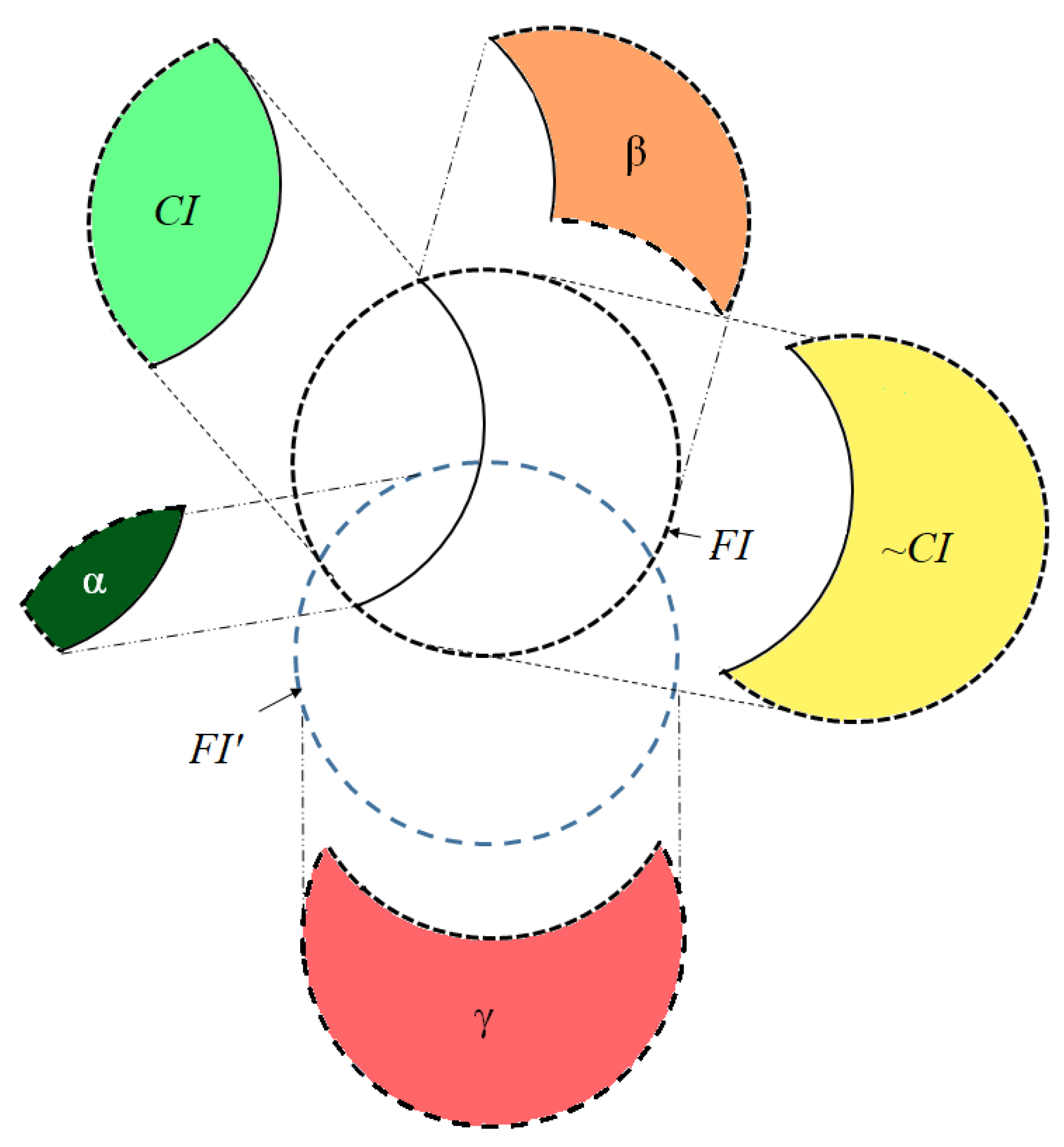
The developed MOPSO-based framework for data sanitization described in this section consists of two steps. For the first data processing step, the frequent itemsets and the pre-large itemsets are discovered and placed into the FIs and PFs sets, respectively, for a later process. Details of this are provided in the next subsection. Moreover, transactions with any confidential information are then projected as a new database for a later process. For the second evolution step, the two updating strategies of gbest and pbest for particles with dominance relationships and the GMPSO algorithm are designed to iteratively update the particles in the evolutionary process. A pre-large concept is also utilized to speed up the evolutionary computation of the execution time. Details of these are as follows.

4.1. Data Processing

Before the sanitization process, the user has to set the confidential information to hidden, and such itemsets are placed in the CI set. The frequent itemsets and the pre-large itemsets are then discovered against the minimum and pre-large support counts, and placed into the FIs and PFs sets, respectively. Because the evolution process requires a certain number of computations, the pre-large itemsets are considered as a buffer to reduce the computational cost in terms of the artificial cost of the side effects in the evolution process. The lower support ($lowsup$) of the pre-large concept is derived as follows:

$$lowsup=\lfloor \frac{minsup\times (|D|-m)}{\left|D\right|}\rfloor \times 100\%,$$

(11)

where $minsup$ is the minimum support threshold, $\left|D\right|$ is the number of transactions in the database, and m is the size of a particle in the designed MOPSO-based framework, which is defined through Equation (5).

Thanks to the discovered large and pre-large itemsets, multiple database scans can be greatly reduced during the evolutionary process. To obtain better transactions for deletion in PPDM, the database is first processed to project the transactions with any of the confidential information appearing in the set of CI. The projected database is then set as $D^{*}$. Each transaction in $D^{*}$ consists of at least one itemset within the set of CI, which is also considered a candidate of the particles for later deletion during the evolutionary process. A detailed algorithm is given in Algorithm 1.

Algorithm 1: Data Processing

In the data processing, the inputs of D and CI are the original database and the set of confidential itemsets, respectively, and the outputs $D^{*}$, FI, and PF are the projected database, the set of large itemsets, and the set of pre-large itemsets. First, the original database is scanned to obtain the FI and PF using minsup and lowsup (line 1), respectively. The algorithm used for mining the FI and PF can be the variants of the pre-large algorithm [45,46]. The transactions containing any of the confidential itemsets are then projected (lines 2–4). The size of each particle is then calculated (line 5) for the later evolutionary process. Thanks to the advantages of the pre-large itemsets, the side effects of the artificial cost can be easily maintained and updated because the potential itemsets that may become large itemsets are kept in PF. Finally, the projected database ($D^{*}$), the frequent itemsets (FI), and pre-large itemsets (PF) are then returned as the outputs (line 6) for the next evolution process.

4.2. Evolution Process

In the second evolution process, the particles are then evaluated to obtain better solutions for the next iteration. In an MOPSO-based framework, each particle can be represented as a possible solution with $MDT$ vectors, and each vector has a transaction ID, which shows the transaction for deletion. Note that a vector in a particle can have a null value. In the updating stage of the evolutionary process, the formulas are thus defined as follows:

$$v_i(t+1)=(pbest-x_i(t))\cup (gbest-x_i(t)),$$

(12)

$$x_i(t+1)=rand(x_i(t),\mathit{null})+v_i(t+1).$$

(13)

In the updating process, the designed GMPSO handles data sanitization in PPDM as a discrete problem. Thus, several parameters used in a traditional PSO are unnecessary in the designed GMPSO. For the updating process, the TIDs within the elder particle or null value are then randomly chosen to fill in the size of the particle, which is shown in Equation (12). The results are then summed with the updated velocity of the particle, which is shown in Equation (13). This method increases the randomization of the exploration ability during the evolution process.

For instance, supposing that the particle size is set as 4, a particle is initially set as $x(t)$ = [1, 2, 5, 8]; gbest is initially set as [0, 4, 0, 5], and pbest is initially set as pbest = [2, 1, 0, 6]. Note that 0 represents a null value, which indicates that a non-transaction is selected for deletion. Thus, the particle can be updated as follows: $v(t+1)$ = {[1, 2, 5, 8] - [2, 1, 0, 6]} ∪ {[0, 2, 0, 5] - [1, 2, 5, 8]} = [5, 8] ∪ [0] = [5, 8, 0]. Because the size of a particle is set as 4, we then randomly select one transaction from its elder content as $rand$(1, 2, 5, 8) (= 1). Thus, the particle is updated as [5, 8, 0, 1].

Because the MOPSO-based framework is used to solve a multi-objective problem, the pbest of each particle cannot be simply determined based on the fitness value. Thus, the non-domination relation is adapted to obtain pbest during the updating process. The local updating strategy is defined as follows:

Strategy 1 (Local Updating Strategy, LUS).

$$pbest\leftarrow \left\{\begin{array}{cc}x(t+1)\hfill & iff(x(t+1))\succ f(\mathit{pbest}),\hfill \\ rand(x(t+1),pbest)\hfill & otherwise.\hfill \end{array}\right.$$

(14)

Thus, if the current particle dominates its last pbest, the pbest can be replaced by the current particle; otherwise, a random selection is then conducted to select a particle as pbest for the next iteration.

To obtain gbest, a global updating strategy is then designed to obtain a better updating solution during the evolution process. Using the designed GMPSO algorithm, a grid-based method is then assigned to a set of candidate particles, and each particle is then assigned with a probability based on the number of grids and the number of the particles in each grid. A random function is then performed to choose one of the candidate particles as gbest based on their assigned probability. The global updating strategy can be stated as follows:

Strategy 2 (Global Updating Strategy, GUS).

$$gbest\leftarrow rand(p_{prob}).$$

(15)

Without loss of generality, the multi-objective optimization problem with n-objectives ($n\ge 2$) to be minimized can be defined as:

$$minf(x)={[f_1(x),f_2(x),\cdots ,f_n(x)]}^T,$$

(16)

which is subject to {$g_i(x)\le 0,i=1,2,\cdots ,n_g$} and {$h_j(x)=0,j=1,2,\cdots ,n_h$}, and $x\in \mathbb{X}$. Moreover, $x\in \mathbb{X}$ is the vector of optimization variables; $\mathbb{X}\subset {\mathbb{R}}^n$ is the optimized domain, which can be defined by the Cartesian product of the domain of each optimization variable. $f(•):\mathbb{X}\mapsto {\mathbb{R}}^m$ is the objective functions of the problem; $g(•):\mathbb{X}\mapsto {\mathbb{R}}^{n_g}$ and $h(•):\mathbb{X}\mapsto {\mathbb{R}}^{n_h}$ represents, respectively, the inequality and equality constraints of the problem. The set of feasible solutions is represented by $\mathrm{\Omega }\subseteq \mathbb{X}$.

Essentially, the goal of multi-objective evolutionary algorithms is to obtain a diverse set of estimates of the Pareto optimal set, which contains the non-dominated solutions of the multi-objective problem. Pareto dominance [47] has been the most commonly adopted criterion used to discriminate among solutions in the multi-objective context, and therefore it has been the basis to develop most of the MOEAs proposed so far. A theorem of Pareto dominance relation is given below.

Theorem 1.

A feasible $x\in \mathrm{\Omega }$ Pareto-dominates another point $x^{\prime }\in \mathrm{\Omega }$ if it holds: $f(x)\le f(x^{\prime })$ and $f(x)\ne f(x^{\prime })$ and the relation operation ≤ and ≠ are defined as: $f(a)\le f(b)\iff f_i(a)\le f_i(b),\forall i\in \{1,2,\cdots ,m\}$, and $f(a)\ne f(b)\iff \exists i\in \{1,2,\cdots ,m\}:f_i(a)\ne f_i(b)$.

The above theorem of a and b respectively represents two different decision vectors. Normally, this dominance is usually presented as: $f(x)\prec f(x^{\prime })$. Based on the theorem of Pareto dominance, the four side effects can be considered as four objects, and the solutions of the optimization in PPDM is to find a set of un-dominated solutions for transaction deletion. Thus, the Pareto dominance can be utilized in the designed algorithm and holds the correctness of the dominance relationships of the derived solutions. The details of the designed GMPSO algorithm are described in Algorithm 2.

Algorithm 2: Proposed GMPSO Algorithm

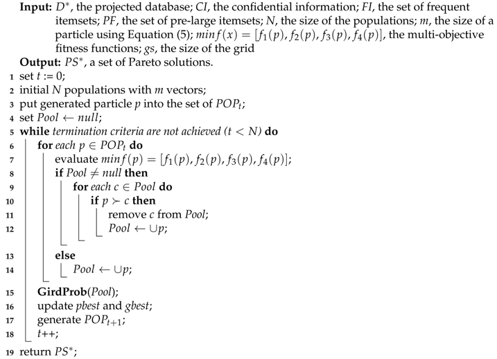
Here, $D^{*}$, CI, FI, PF, and N are the projected database, the set of confidential information, the set of large itemsets, the set of pre-large itemsets, and the number of populations, respectively. In addition, $f_1$, $f_2$, $f_3$, and $f_4$ are four fitness functions presenting the number of hiding failures, the missing cost, the artificial cost, and the number of database dissimilarities, (Dis), respectively First, N particles are randomly initialized as m vectors based on the size of each particle (line 1). The generated particles are then put into the set of $PO{P}_0$ as the initial populations. The candidate set of the Pareto front is then set as null (line 4). Next, an iterative process is then applied until the termination criteria are achieved, for example, the number of iterations ($t<N$, lines 5–18). Each particle in the candidate set of the Pareto front is then evaluated using four fitness functions (line 7) to find the non-dominated solutions (lines 8–14). The satisfied solutions are then applied using the GridProb function to assign the probability of each particle in the grid. The pseudo-code of the GridProb function is illustrated in Algorithm 3.

Algorithm 3: GridProb(Pool)

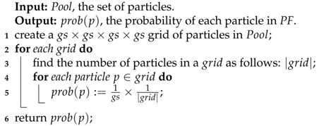
In Algorithm 3, the size of the grid is initially set based on user preference. For each grid, the number of grids can be found using $\left|grid\right|$ (line 3), and the probability of each particle within a grid is then calculated (line 5). Each particle then receives a probability for later selection of gbest, which increases the diversity of the solutions. To clearly explain the abbreviations used in this paper, the explantions of all acronyms are shown in the Appendix A section.

5. An Illustrated Example

In this section, we illustrate a simple example to explain the designed algorithm step-by-step. In this example, the original database was shown in

Table 1. The original database.

TID	Items	TID	Items
$T_1$	A, B, E	$T_6$	B, C, E
$T_2$	B, C, E	$T_7$	B, C, D, E
$T_3$	A, B, C, E	$T_8$	A, B, E
$T_4$	A, C, D	$T_9$	A, B
$T_5$	B, C, E	$T_{10}$	C, E

, and the upper support threshold (minimum support threshold) is initially set as 35%. The discovered frequent itemsets are then shown in

Table 2. The discovered frequent itemsets.

1-Itemset	Count	2-Itemset	Count	3-Itmset	Count
(A)	5	(AB)	4	(BCE)	5
(B)	8	(BC)	5
(C)	7	(BE)	7
(E)	8	(CE)	6

.

Assume that itemsets (AB) and (BC) from Table 2 are the sensitive itemsets. At the beginning, it would be better to calculate the at least number of transactions to be deleted to completely hide sensitive itemsets. According to Equation (4) and Equation (5), we then have an m value as 4, and the lowsup is calculated by Equation (11) as 24%. Based on the lowsup, we can find the support count of pre-large itemset as 10 × 24% (= 3). The pre-large itemsets are used to reduce the computational cost of multiple database scans. In this example, the pre-large itemsets are {(AE):3, (ABE):3}.

Afterwards, the transactions containing any of confidential information is then projected, which will be used as the transactions to be deleted in the evolutionary progress. In this example, the projected database is shown in

Table 3. The projected database.

TID	Items
$T_2$	B, C, E
$T_3$	A, B, C, E
$T_5$	B, C, E
$T_6$	B, C, E
$T_7$	B, C, D, E
$T_{10}$	C, E

.

Thus, only the transactions {$T_2$, $T_3$, $T_5$, $T_6$, $T_7$, $T_{10}$} can be considered as the transactions for deletion in the sanitization process. Due to m equaling 4, the size of a particle is 4. Assume the size of a particle is set to 4 and the initial populations for the evolutionary process are randomly chosen from Table 3. After that, the particles of the populations are then evaluated one-by-one based on the defined multi-objective functions shown in Equation (10). Take the particle $P_1$, for example, to illustrate the evaluation process. Suppose the $P_1$ selects the transactions {$T_2$, $T_3$, $T_5$, $T_6$} for transaction deletion to hide the sensitive itemsets for sanitization. Thus, the supports of (BC) and (CE) respectively become (1/6 = 16.7% < 35%), and (2/6 = 33.3% < 35%); the (BC) and (CE) are then completely hidden after the sanitization process. Moreover, the $f_1$ (hiding failure) of the particle is calculated as 0. The discovered frequent itemsets in Table 2 are then updated. In this example, the non-sensitive itemset of (BCE) becomes (1/6 = 16.7% < 35%), which will be hidden after the sanitization progress. The missing cost of $f_2$ is returned as 1. Since the artificial itemsets can be generated from the pre-large itemsets, in this example, none of the itemsets are generated as the artificial cost. The artificial cost of $f_3$ is returned as 0. The Dis is calculated as 4 because four transactions are deleted from the database for sanitization. All the particles are then evaluated in the same way, and the results after evaluation are shown in

Table 4. The initial population.

Particle	TIDs	${\mathit{f}}_1$	${\mathit{f}}_2$	${\mathit{f}}_3$	${\mathit{f}}_4$
$P_1$	2, 3, 5, 6	0	1	0	4
$P_2$	0, 5, 6, 7	1	1	2	3
$P_3$	0, 2, 3, 3	1	1	1	3
$P_4$	0, 5, 6, 0	1	0	1	2
$P_5$	2, 3, 0, 10	2	0	0	3

.

After that, we then find the non-dominated particles of population. It is clear that the $P_1$, $P_4$ and $P_5$ are the non-dominated particles in this running example based on the non-dominated property. Based on the grid method, we then can assign the probability of each particle for the updating of gbest (global best). In this example, suppose $P_4$ is selected as the candidate for the updating process. We also take $P_3$ as an example to illustrate the evolution process step-by-step. We first calculate the position and velocity of the particle by Equation (12) and Equation (13). The velocity is then calculated as as {[0, 2, 3, 3] - [0, 2, 3, 3]} ∪ {[0, 5, 6, 0] - [0, 2, 3, 3]} = {null∪ [5, 6]} = [5, 6]. Since there are two empty dimensions in the updated particle, we select two values randomly from the elder particle (or null). Assume we then randomly select rand([0, 2, 3, 3], 0) = [0, 2] for two dimensions; thus, the update particle is [0, 2, 5, 6]. After that, we then evaluate the side effect values of all updated particles based on the multi-objective functions. The same procedure then iteratively performs until the number of generation is achieved. After that, we then obtain a set of non-dominated results as the final solution for data sanitization.

6. Experimental Results

Several experiments were carried out to compare the effectiveness and efficiency of the proposed GMPSO algorithm to the state-of-the-art single-objective cpGA2DT [19] and NSGA-II-based [23] approaches. The algorithms used in the experiments were implemented in Java, using a PC with an Intel Core i7-6700 quad-core processor and 8 GB of RAM under the 64-bit Microsoft Windows 10 operating system. Three real-world datasets [48], called chess, mushroom, and foodmart, were used in the experiments. Because the foodmart dataset originally consisted of items and their purchase quantities, only the distinct items in the foodmart dataset were extracted and used in the experiments. A synthetic dataset, namely, T10I4D100K, was also generated using the IBM database generator [49] for the experiments. The characteristics of the datasets used in the experiments are shown in

Table 5. Characteristics of datasets used.

Dataset	$\#\left|\mathbf{D}\right|$	$\#\left|\mathbf{I}\right|$	AvgLen	MaxLen	Type
chess	3196	74	37	37	dense
mushroom	8124	119	23	23	dense
foodmart	21,556	1559	4	11	sparse
T10I4D100K	100,000	870	10.1	29	sparse

. The used parameters are defined as: $\#\left|\mathbf{D}\right|$: the total number of transactions; $\#\left|\mathbf{I}\right|$: the number of distinct items; AvgLen: the average transaction length; MaxLen: the maximal length transactions; and Type: The dataset type.

The maximum number of iterations is set to 50 and population size is set to 50 in the experiments for all the compared algorithms. All the experiments are conducted five times and the average values are calculated. The single-point crossover and bit-wise mutation are then performed and the rates are respectively set to 0.9 and 0.01 for the cpGA2DT algorithm. The elitism method is used in the cpGA2DT algorithm to select populations. The results in terms of the runtime, four side effects, and the scalability are discussed and analyzed as follows.

6.1. Runtime

During the experiments, the execution time under varying percentages of sensitivity with a fixed minimum support threshold was determined for the four datasets. In this section, only the NSGA-II-based model is compared with the designed GMPSO because it is unreasonable to compare a single-objective algorithm with multi-objective algorithms. The results of the two multi-objective algorithms are shown in Figure 3.

It is clear that the designed GMPSO consumes remarkably less runtime than the NSGA-II-based model under varied percentages of sensitivity of frequent itemsets. The reason for this is because the NSGA-II-based model spends a lot of time on generating new populations using crossover and mutation operations. The sorting strategy of the Pareto solutions in the NSGA-II-based model also requires some computational time. However, the presented GMPSO algorithm does not require crossover and mutation operations to generate the next populations. The results in terms of the four side effects are then shown.

6.2. Side Effects

In this section, the state-of-the-art single-objective cpGA2DT [19] and multi-objective NSGA-II-based model [23] are then compared to the designed GMPSO in terms of the hiding failure ($\alpha$), missing cost ($\beta$), artificial cost ($\gamma$) and database dissimilarity (Dis). The number of populations for all evolutionary algorithms is set to 50. Because a multi-objective algorithm will produce a set of Pareto-front solutions, we evaluated the side effects based on the average of the produced solutions. The results of hiding failure for the four datasets are shown in Figure 4.

From Figure 4, we can clearly see that the designed GMPSO reaches a lower side effect in terms of hiding failure, which indicates that most confidential information is hidden after the sanitization process. For example, when the percentage of sensitivity is set as 4% for the chess dataset, the hiding failures of cpGA2DT, the NSGA-II-based model, and the designed GMPSO are 50, 52.5, and 25, respectively, which indicates that the GMPSO achieves the lowest hiding failure compared with the other approaches. When the percentage of sensitivity is set as 6% for the foodmart dataset, the designed GMPSO has no side effects in terms of a hiding failure, nor does the NSGA-II-based model. The results of GMPSO under the chess and mushroom datasets outperform the results under the foodmart and T10I4D100K datasets. This is reasonable because the chess and foodmart datasets belong to a dense dataset, and most itemsets have a high relevance to each other, and thus the contents of the transactions even have a high overlap. Therefore, the deleted transactions may have high overlap of confidential information; more confidential information can be deleted together and a lower hiding failure can be achieved. We then applied the results of missing cost, as shown in Figure 5.

From Figure 5, it can be seen that the GMPSO occasionally achieves a higher missing cost under the chess and mushroom datasets, the reason for which is that these two datasets belong to a dense dataset; in addition, the contents of most transactions have a high overlap. Thus, when more confidential information is deleted from the dataset, more discovered information may be deleted together. Based on the results shown in Figure 4a,b, we can see that the GMPSO achieves the lowest hiding failure than the other algorithms. Thus, the GMPSO occasionally produces a higher missing cost in very dense datasets. However, for spare datasets such as foodmart and T10I4D100K shown in Figure 5c,d, respectively, the designed GMPSO produced no missing cost under varied percentages of sensitivity of frequent itemsets compared to the cpGA2DT and NSGA-II-based model. From Figure 4c,d, we can see that the GMPSO occasionally has no hiding failure and achieves almost optimized solutions as compared to the cpGA2DT and NSGA-II-based model; we then concluded that the GMPSO achieves a good performance in terms of the missing cost. The results of the artificial cost are shown in Figure 6.

From Figure 6, we can see that GMPSO generates a higher artificial cost than cpGA2DT and the NSGA-II-based model for very dense datasets such as chess and mushroom, as shown in Figure 6a,b. The reason for this is that, when more of the hiding failure is prohibited, as the results in Figure 4a,b show, for example, the size of the database is reduced; more unexpected rules then arise as new information after the sanitization process owing to the change in threshold. This is reasonable because there is a trade-off relationship between the hiding failure and artificial cost. For sparse datasets such as foodmart and T10I4D100K, none of the algorithms, including GMPSO, generate any artificial costs; the three compared algorithms achieve the optimized results in terms of the artificial cost for sparse datasets. The results of the database similarity (Dis) are then applied, as shown in Figure 7.

From Figure 7, we can see that the NSGA-II-based model achieves the best Dis compared to the other two algorithms. The reason for this is that, based on Figure 4a,b, the NSGA-II-based model achieves worse results in terms of hiding failure; less information is then deleted and thus the side effect of Dis is not high. As we can see, the proposed GMPSO achieves a good performance in terms of the hiding failure, as shown in Figure 4a,b; more confidential information is deleted and the Dis value is thus increased. For sparse datasets such as foodmart and T10I4D100K, shown in Figure 7c,d, Dis for cpGA2DT, the NSGA-II-based model, and GMPSO is not higher, with a difference of less than 1%; GMPSO can thus show a good performance in terms of Dis. In summary, the designed GMPSO can achieve a good performance in terms of the four side effects and obtain optimized solutions compared to the other two approaches. Moreover, the designed GMPSO shows better flexibility than the single-objective cpGA2DT algorithm because the transactions for deletion can be selected based on user preference.

6.3. Scalability

We then evaluate the scalability of the compared algorithms in terms of database size. The results are shown in Figure 8. In Figure 8a, we can see that all compared algorithms almost achieve the same results expect the cpGA2DT algorithm under T10I4D150K dataset. The NSGA-II and the designed GMPSO have the same results for hiding failure. However, in Figure 8b, the designed GMPSO generates nothing of missing cost from the dataset size 100 K to 250 K, and increments 50 K each time. Moreover, the GMPSO has no artificial cost under the dataset T10I4D150K, but the cpGA2DT and NSGA-II still generate the side effect of artificial cost under the dataset T10I4D150K. Since it is a trade-off relationship between four side effects, the designed GMPSO somehow generates a slight database dissimilarity (Dis) compared to the other two algorithms, for example, under the dataset T10I4D100K. However, it only has 0.05% difference of the Dis compared to the other two algorithms. In general, the designed GMPSO still has obtained good effectiveness in terms of four side effects compared to the cpGA2DT and NSGA-II algorithms in terms of scalability.

7. Conclusions and Areas of Future Study

In this paper, we first presented a grid-based multi-objective particle swarm optimization algorithm (called GMPSO) for data sanitization in the area of privacy-preserving data mining. Two updating strategies are utilized to find the better diversity of the obtained solutions. The pre-large concept is also utilized in this study to speed up the computations. From the results, we can see that the designed GMPSO achieves a good performance in terms of hiding confidential information (hiding failure), and occasionally obtains optimized results in terms of the missing and artificial costs. Because a trade-off relationship exists between the side effects, the GMPSO still obtains a minor side effect of database dissimilarity (Dis) compared to cpGA2DT and the NSGA-II-based model. In summary, the designed GMPSO achieves a good performance in terms of four side effects and provides higher flexibility than the other two algorithms.