Review

A Comprehensive Survey of Accurate and Efficient Aggregation Modeling for High Penetration of Large-Scale Wind Farms in Smart Grid

1
School of Information Science and Engineering, Central South University, Changsha 410083, China
2
School of Automation, China University of Geosciences, Wuhan 430074, China
*
Author to whom correspondence should be addressed.
Appl. Sci. 2019, 9(4), 769; https://doi.org/10.3390/app9040769
Submission received: 14 December 2018 / Revised: 28 January 2019 / Accepted: 18 February 2019 / Published: 22 February 2019

Abstract

:
As one of the important renewable energies, wind power has been exploited worldwide. Modeling plays an important role in the high penetration of wind farms in smart grids. Aggregation modeling, whose benefits include low computational complexity and high computing speed, is widely used in wind farm modeling and simulation. To contribute to the development of wind power generation, a comprehensive survey of the aggregation modeling of wind farms is given in this article. A wind farm aggregation model consists of three parts, respectively, the wind speed model, the wind turbine generator (WTG) model, and the WTG transmission system model. Different modeling and aggregation methods, principles, and formulas for the above three parts are introduced. First, the features and emphasis of different wind speed models are discussed. Then, the aggregated wind turbine generator (WTG) models are divided into single WTG and multi-WTG aggregation models, considering the aggregation of wind turbines and generators, respectively. The calculation methods for the wind conditions and parameters of different aggregation models are discussed. Finally, the WTG transmission model of the wind farm from the aggregation bus is introduced. Some research directions are highlighted in the end according to the issues related to the aggregation modeling of wind farms in smart grids.

1. Introduction

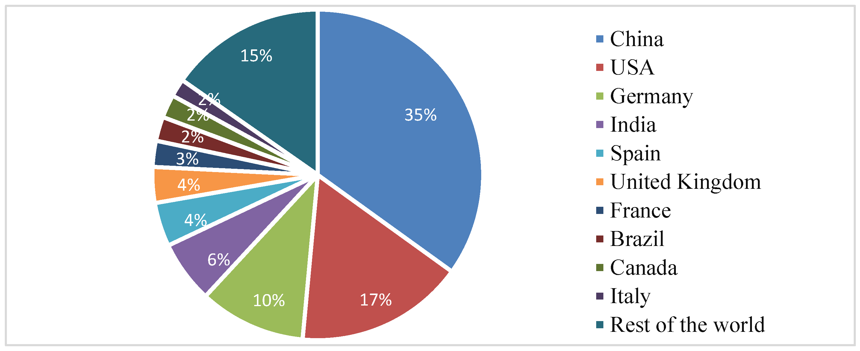
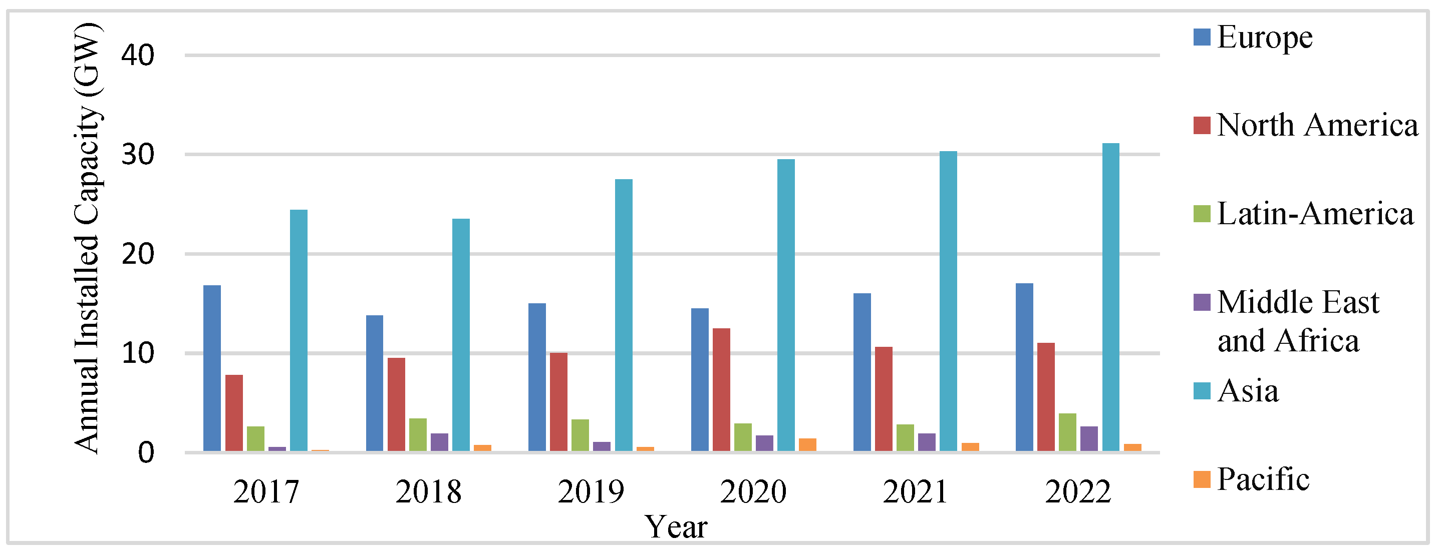
In light of increasing of energy crises and environmental pollution, the utilization of renewable energies is attracting more and more attention. Wind power has been rapidly exploited worldwide due to its low environmental impact and technical development, and expects to reach 2000 GW by the year 2030 [1]. Based on the statistics of the Global Wind Energy Council, the global installed capacity of wind power from 1997–2017 is shown in Figure 1 [2]. The global wind capacity has expanded from 7.6 GW to 539.58 GW in the past two decades, and wind power has experienced a rapid growth trend since 2008. The top 10 countries for total wind power capacity in 2017 can be found in Figure 2 [2]. China, with a total wind power capacity of 188.39 GW, accounts for the largest proportion, with 35%. The United States (89.07 GW, 17%) and Germany (56.13 GW, 10%) take the second and the third place, respectively. Figure 3 shows the prediction of wind power capacity in different areas [2]. Asia is expected to have the fastest development regarding both capacity and developing speed, while Europe and North America are ranked second and third, respectively.
Wind energy is a major part of the smart grid. In the past decades, there are many engineering applications of wind power generation in smart grids [3,4,5,6,7,8,9,10,11], which promotes the progress of related technologies, such as wind farm planning, grid-connected system protection, wind power forecasting and monitoring, and wind farm modeling and simulation.
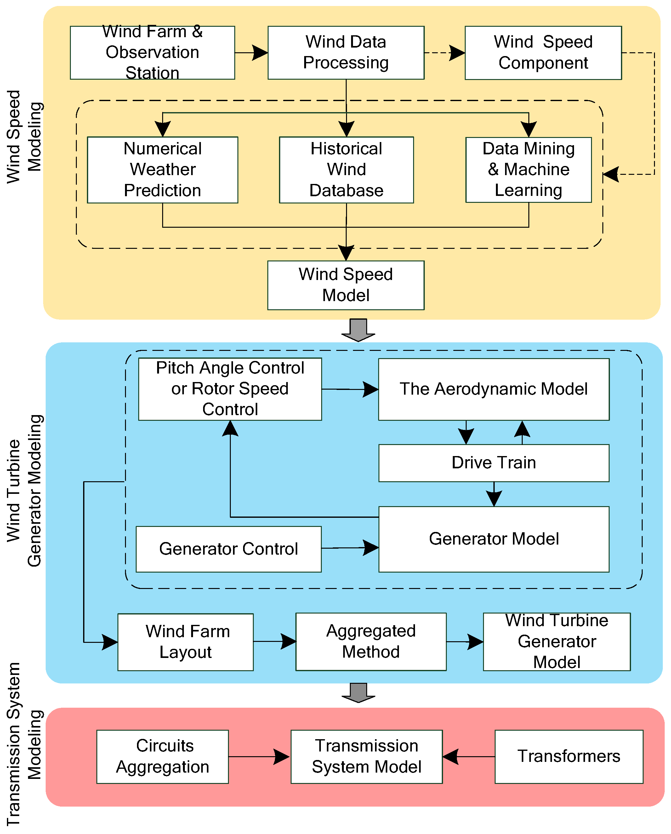
Modeling plays an important role during development. In the early phases, the modeling of a single wind turbine has received more attention, due to the application of small-scale wind power. In recent years, with the advent of new types of wind generators as well as the high penetration of wind power, the modeling and simulation of wind farms has become a research direction in smart grids [12,13,14,15,16,17,18,19]. At present, there are two categories of modeling methods, respectively, (a) detailed modeling, and (b) equivalent modeling. In detailed modeling, all of the components, such as generators, step-up transformers, and a large number of collector circuits, are modeled comprehensively. However, equivalent modeling starts from the influence of wind farms on smart grids, and regards wind farms as a whole to aggregate or reduce the order of wind turbines. Compared with detailing modeling, equivalent modeling is used widely, since its computational complexity is drastically reduced, while legitimate precision is maintained. Figure 4 shows the framework of the wind farm modeling with the aggregating method.
The wind farm aggregation modeling mainly consists of the following three stages.
(1) Modeling of wind speed. Randomness, volatility, and uncontrollability are the main aspects of wind speed that affect the operation and grid-integration of wind farms. Based on the features and emphasis, wind speed models include three groups: probability distribution models, time-series models, and component models. Probability distribution models and data-based black box models are established by the large amounts of data, including measured wind speed, historical data, wind speed prediction, and environment data. In the component model, wind speed is decomposed into different wind speed components focusing on different wind speed variety characteristics and different time lengths. Then, the probability distribution model or time-series wind speed model for each wind speed component can be established.
(2) Modeling of wind turbine generator. The wind turbine generator (WTG) model is the key part of the aggregation modeling of a wind farm. The wind turbines have experienced an improvement from the squirrel-cage asynchronous to the doubly-fed induction generator (DFIG) wind turbine, and then to the direct-driven permanent magnet synchronous generator (D-PMSG) wind turbine. Different types of wind turbine generators have different physical and electromagnetic structures. When establishing a single wind turbine generator, the wind turbine-driven train system, generator, electronic devices, as well as control system should be considered. Meanwhile, the scale of the wind farm, the distribution of wind turbines, the turbine types, and the research target should be considered comprehensively when aggregating the wind farm into a multi-machine aggregation model.
(3) Modeling of WTG transmission aggregation. The layout of wind farms, the size and type of conductors, and the delivery method (overhead or buried cables) all have an influence when computing the aggregated output of a wind farm at its aggregation bus [20,21]. As the scale of the wind farm is expanded, the computation complexity increases. The aggregation of the WTG transmission is useful not only for simplifying the equivalent model, but also for wind farm expansion planning.
The objective of this paper is to give a understanding of recent aggregation modeling methods for wind farms, including the modeling of wind speed, WTG, and the transmission system inside a wind farm. Different models or modeling methods, as well as their characteristics and applications, are reviewed, which could help researchers in dealing with wind farm aggregation modeling issues.
The remaining sections of this paper are structured as follows. In Section 2, different types of wind speed models are introduced. In Section 3, the wind turbine and the generator are considered as the two major parts of the WTG. A single-machine model and multi-machine model of different wind turbine generators are discussed. The WTG transmission system modeling method is introduced in Section 4, and the conclusion is drawn in Section 5.

2. Wind Speed Modeling

2.1. Probability Distribution Model

The probability distribution modeling is a data-based method that extracts characteristics in a statistical way to depict the probability distribution of wind speed. It reflects the expectations of wind speed over a period of time, and provides guidance for wind resource assessment. It can be classified into parameter distribution models and non-parameter distribution models.

2.1.1. Parameter Distribution Model

In the parameter distribution model, wind speed is presupposed to be effectively described by probability density functions based on historical wind data. The probability density function can be either a single function or a combination of two or more functions. Weibull distribution, Rayleigh distribution, and normal distribution are the widely used single distribution functions [22,23,24,25]. More specifically, the wind speed modeling by using Weibull distribution mainly has the following steps [23,24].
Step-1. Assuming that the measured wind speed sequence (v1, v2, …, vn) obeys the two-parameter Weibull distributions, i.e.,:
F ( V ) = P ( ν V ) = 1 exp [ ( V / c ) k ]
f ( V ) = ( k / c ) ( V / c ) k 1 exp [ ( V / c ) k ]
where c and k are the scale and shape parameter of the Weibull distribution, respectively, and c reflects the average wind speed of wind farm; V is the given wind speed m/s.
Step-2. The maximum likelihood method is used to construct the logarithm likelihood function:
L ( k , c ) = i = 1 n [ ln k + ( k 1 ) ln V i k ln c ( V i / c ) k ]
Let the gradients F 1 = L ( k , c ) k = 0 , and F 1 = L ( k , c ) c = 0 , then:
F 1 = i = 1 n [ 1 / k + ln V i ln c ( V i / c ) k ln ( V i / c ) ] = 0
F 2 = i = 1 n [ c / k + ( k / c ) ( V i / c ) k ] = 0
Step-3. The initial values of c and k are selected. After using the iterative algorithm to find the optimal values that satisfy the convergence criterion max {|Δk, Δc|}≤ε, where ε is a preset small positive value, the Weibull probability distribution model is obtained.
The X2 test and the Kolmogorov–Smirnov test, which creates a relatively small error when a theoretical parameter distribution is rejected, are usually used to evaluate the precision of the parameter distribution model. The two tests reflect relative percentages, and can be added together. A larger unified metric value represents a worse goodness-of-fit. Other indexes, such as square error and mean-square-root error, are also available for precision evaluation [25].

2.1.2. Non-Parameter Distribution Model

As we know, parameter distribution models assume that wind speed can be described by a probability density function. However, when the assumption does not coincide with the actual distribution, the calculation error is inevitably increased. In recent years, non-parameter distribution models of wind speed are proposed to solve the errors between the probability density function and actual wind distribution, and are suitable for analyzing the feature space of arbitrary structures.
A typical non-parameter distribution model of wind speed based on non-parametric kernel density estimation is proposed in [26,27]. Neither prior knowledge of wind speed data nor any hypothesis of probability distribution form is required. The model consists of the following steps:
Step-1. Selecting the sampling sequences of wind speed;
Step-2. Establishing the wind speed probability density function; and
Step-3. Selecting the kernel function and smooth parameters to establish the wind speed model.
Assuming the sampling sequence of wind speed is (v1, v2, …, vn) and the probability density function of wind speed is f(v), the kernel density estimation can be expressed as:
f ^ ( v ) = 1 n h i = 1 n K [ ( v 1 v i ) / h ]
where n is the sampling size; h is the window width, which is also called smoothing parameter; and K(·) is the kernel function. When the sampling size is large enough, the selection of kernel function has a limited influence on the result, and vice versa. Special attention must be paid to the selection of the optimal smoothing parameter hopt, since the smooth parameter has a great influence on the estimation accuracy of the kernel density.
The asymptotic integrated mean squared error (AIMSE) consists of bias and variance, and is a commonly accepted criterion to quantify the estimation error in a kernel density model [27]. The minimization of AIMSE means choosing an appropriate bandwidth that can achieve good balance between bias and variance, and ensuring that neither is too small or too large.

2.2. Data-Based Black Box Model

Measured and historical data of wind speed, wind speed prediction by the local meteorological center, and other measured environment data are used to build the black box model of wind speed by data-driven modeling methods. A time-series wind speed model is a kind of data-based black box model that depicts the dynamic changes of wind speed over time by using historical wind speed data. This model is the precondition of wind power integration reliability assessment in the planning stage, and the first link in wind power credible capacity evaluation [27,28,29,30,31,32]. Autoregressive (AR), moving average (MA), autoregressive moving average (ARMA), and autoregressive integrated moving average (ARIMA) are the methods to build a time-series model. The literatures [28,29] using an ARMA model to fit the wind speed spectrum function and to establish the wind speed model. The literature [14] has applied a time-series modeling theory based on a higher-order statistics method. The reconstructed ARMA model for a short time series performs good robustness and high precision.
The Markov random process model is another kind of data-based black box model. Based on the statistical analysis and transition probability calculation, the wind speed can be obtained [27]. A discrete-state Markov chain model (DSMC), continuous state model, and birth-and-death Markov process model are the commonly used Markov random process models. As representatives of these two types of models, the ARMA model and DSMC model are compared, as shown in Table A1. In addition to the aforementioned models, many data-driven methods, such as neural network and support vector machine, combined with multi-source data, are used to build black box models of wind speed [33,34,35].

2.3. Component Model

Component models provide another perspective on wind speed analysis. Wind speed is decomposed into different wind speed components based on the wind speed variety characteristics and time length. Two-component wind speed models and four-component wind speed models are the commonly used. Models of each wind speed component can respectively established based on the probability distribution or time-series data. In a two-component wind speed model, wind speed is the superposition of the average wind speed component and the wind turbulence component. The two-component wind speed model is widely used in time-series wind speed models [27,28]. In this model, the instantaneous wind speed V(t) can be expressed as:
V ( t ) = V ¯ + V ( t )
where V ¯ is the average component, and V ( t ) is the turbulence component.
In Equation (7), the average wind speed component can be expressed as:
V ¯ = 1 t 2 t 1 t 1 t 2 V ( t ) d t
According to the wind profile, the average wind speed can be described with the following logarithmic distribution or exponential distribution:
V ¯ ( z ) = ( V * / k ) ln ( z / z 0 )
V ¯ ( z ) V ( Z s ) = ( z / z s ) α
where z is the height from the ground; z0 is the roughness length of the ground surface; V* is the friction velocity; Zs is the reference height from the ground; k is the Karman constant; and α is the wind profile index.
In Equation (7), the wind turbulence component is mainly described by wind spectrum and correlation functions. A commonly used Davenport spectral density function is:
S ( f ) = 4 K V ¯ ( 10 ) 2 ( 1200 f / V ¯ ( 10 ) ) 2 f [ 1 + ( 1200 f / V ¯ ( 10 ) ) 2 ] 4 / 3
where S(f) is the spectral density function at frequency f, and K is the roughness coefficient of the ground. In the Davenport spectral, the reference height is chosen to be 10 meters.
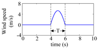
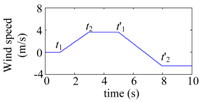
A four-component wind speed model using basic wind, gust wind, gradient wind, and random wind is used to describe the different characteristics of wind speed. The description of the four-component wind speed model is shown in Table A2, and the comparison between the two-component and the four-component model is shown in Table A3. In [32], a more accurate four-component wind speed model is proposed to simulate the effects of terrain and time delay on wind speed. Two coordinate transformation matrices are used to consider the wind direction factor. The wake effect of wind turbine generators on the wind-speed distribution is considered in the proposed model.

3. Wind Turbine Generator Model

3.1. Types of Wind Turbine Generator

The wind turbine generator is the basic unit of a wind farm. The pitch angle system, driven train, generator, and their corresponding control systems are the major parts of the WTG model. Different types of WTGs have different physical and electromagnetic structures. When modeling a wind farm, the type of WTG should be considered in advance. The three types of WTGs that are mainly used in wind farms are a squirrel-cage induction generator (SCIG), double-fed induction generator (DFIG), and direct-driven permanent magnet synchronous generator (D-PMSG) [36]. The structures of these WTGs are respectively shown in Figure 5.
Different WTGs have different configurations and need to be modeled with different methods. Here, we present some typical modeling processes for these WTGs. The comprehensive mathematical model of the WTGs can be found in [36,37,38,39,40,41].
(1) SCIG: The typical modeling of a SCIG can be carried out by the following steps [37,38]. First, the wind farm is set with a constant speed. Then, the rotor speed of the wind turbines is selected after the fault as the clustering indexes [36,38]. Finally, WTGs are divided into different units with the K-means clustering algorithm. Once the output power, the terminal voltage, and the fault duration time are determined, the clustering index τ can be calculated accordingly as:
τ = 1 + U 2 r 2 U 4 r 2 2 4 P m 2 ( x 1 + x 2 ) 2 r 2 2 2 P m ( x 1 + x 2 ) 2 + T m K s a t c + T m K s b sin ( t c ) 2 H g c
where a = Hg/(KsHt + KsHg), b = Ht/(KsHt + KsHg), and c = KsHg(Ht + Hg)/2HtHg; Ht and Hg are the rotor inertial time constant of the wind turbine and the generator, respectively; Tm is the mechanical torque of the wind turbine; Pm is the mechanical power; Ks is the shafting stiffness coefficient; x1 and x2 are the stator reactance and the rotor reactance of generator, respectively; r2 is the rotor resistance; s is the slip; U is the terminal voltage; and t is the failure duration.
(2) DFIG: The DFIG permits speed ranges from 75% to 125% of the synchronous speed. The control strategies of the DFIG is complex, and there are various converters and controllers with a lot of parameters.
(3) D-PMSG: Without a variable speed gearbox, the D-PMSG can avoid the possibility of operation and maintenance problems. The advantages of D-PMSG wind turbines include their wide adaptive range of wind speed, and the simple but flexible control of active and reactive power. Due to the fault isolation feature of the full-scale power converter, the generator and the generator side converter can be ignored when analyzing the system transient states, and only aggregate the grid side converters and their control systems [36,39,40].
The SCIG is the earlier designed WTG, and is usually installed in small-scale wind farms. The DFIG is one of the most widely installed WTGs due to its higher capability, lower investment, and flexible control. In recent years, the D-PMSG has undergone rapid development, especially in offshore wind farms.

3.2. Single WTG Aggregation Model

When all the generators of a wind farm are aggregated to one generator, the wind farm is represented by a single WTG aggregation model. The single WTG aggregation model can be considered as a “single wind turbine + single generator” model, or a single WTG aggregation model for short. In a single WTG aggregation model, all wind turbines as well as generators are respectively aggregated to one wind turbine and one generator. Parameters of various units, such as the capacity, the active power, and the mechanical power of the wind turbines and the generators are aggregated as the parameters of the equivalent wind farm. The process of the aggregation is shown in Figure 6.
In a single WTG aggregated model, there are two kinds of aggregation methods [41]. One aggregates wind turbines with equivalent incoming wind. When winds are different, the average wind speed of individual winds has been used as the equivalent wind. The other aggregates wind turbines along with generators with variable equivalent compensating capacitors to approximate the WTGs under different wind speed situations. The literature [42] has obtained the wind speed input of wind turbines according to the power coefficient curve and their coordinate positions, which is suitable for all wind farms, regardless of the number of wind turbines.
Since all the WTGs are aggregated to a single WTG, the equivalent aggregation modeling of wind farms can be considered as part of the modeling of a WTG, where the WTG types are considered the main aspect, and the other working conditions are considered as secondary.
The literature [43] has proposed an aggregated DFIG model based on a third-order quasi-sinusoidal model with simplifications of the transformer voltage and the grid-side converter. The literature [40] has taken the D-PMSG as an example, and established the single aggregation model by using the volume-weighted method. The performance comparison between the detailed model and multi-machine aggregation model is made to validate the practicability of the aggregating method. The literature [44] proposed an aggregated method of D-PMSG-based wind farms. It points out that the D-PMSG wind turbine has three operating regions: the variable speed operating region, the constant speed, the variable power operating region, and the constant power and variable pitch-angle operating region, where γ1, γ2, and γ3 are used to represent the operating characteristics. The clustering index γ can be defined as follows:
γ = ( γ 1 , γ 2 , γ 3 )
where γ1 = Ωr/Ωmax, γ2 = (Cp/λ3)/(Cp/λ3)max, γ3 = β/βmax; Cp is the utilization efficiency of wind energy; λ is the tip speed ratio of wind turbines; Ωr is the wind rotor speed; and β is the pitch angle. This aggregation method reflects all of the operating characteristics of D-PMSG wind turbines.
The literature [39] takes the pitch–angle control actions of WTGs as the clustering principles, and uses the support vector machine to cluster WTGs. The aggregation contains initial speed, mechanical torque, electromagnetic torque, and the feature vector reflecting the pitch angle control action. The literature [45,46] gives a type of wind farm model that portrays the capability of set-point tracking under intermittent wind conditions. The characteristics of this model in depicting the set-point operation under the automatic generation control are also proved by simulation.
A single WTG aggregation model generally adopts the capacity-weighted average method to calculate the equivalent parameters. The aggregated parameters are expressed as:
δ i = S i / i = 1 N S i
{ S e q = i = 1 N S i , P e q = i = 1 N P i ,      X e q = i = 1 N δ i X i C e q = 1 N i = 1 N C i , A e q = i = 1 N A i , V e q = ( 1 / A e q C e q i = 1 N A i C i V i 3 ) 1 / 3
where S is the capacity of wind turbines; δ is the weighting coefficient of capacity; X is the parameter of the generator; and A, C, and V are the wind area, wind energy utilization coefficient, and wind speed, respectively.
Capacity weighted is a simple multiplier progress with relatively low accuracy. Some improved models, such as the improved equal weighted model and the reduced-order variable-scale equivalent model, are used instead to improve the accuracy [47]. Meanwhile, artificial intelligence can be introduced to improve the accuracy of the single WTG aggregation, and to calculate the aggregation parameters [48,49,50,51].
The single WTG model is a good choice when it meets the accuracy requirements. However, when the working conditions or control parameters of different WTGs are large, the single aggregation model will have large errors. The error introduced by single aggregation model may lead to protection misoperation, followed by a series of abnormal chain reactions. Besides, a single WTG aggregation model cannot be used when a wind farm consists of different types of WTGs.

3.3. Multi-WTG Aggregation Model

The wind turbine and the generator are the two major parts of a WTG. When aggregation modeling WTGs, these two parts can be respectively aggregated. The multi-WTG aggregation model is suitable for wind farms with constant or variable speed.

3.3.1. Aggregation of Wind Turbines

When wind conditions, land form, wake effect, and time delay for different wind turbines are respectively considered, wind turbines are firstly divided into several different regions, and then wind turbines in the same region are aggregated into one wind turbine. The simplified process of this aggregation is shown in Figure 7.
Wind turbine aggregation is appropriate for the dynamic modeling of the wind farms when the differences in working conditions are large. The literature [52,53] has pointed out that this model has some restrictions in the application of simulation because of its inherent structure changes.
Due to the wake flow, the input speed of the downstream turbine is lower than that of the upstream turbine. The main factors of wake effect are the distances between wind turbines, the characteristics of thrust and power, and the turbulence intensity. The energy fluctuations could range from 2% to 30%. The wake effect is generally described by the Lissaman model and the Jensen model. The Jensen model simulates the wake effect in a flat area, and the Lissaman model simulates a non-uniform wind field. Sometimes, these two models are combined and used to deal with complex terrain. The literature [42] discusses three models of wake effect, where the wind shade, shear effect, and wind direction are considered. In [54,55], the wake effect models of flat or complex terrain are introduced.
Regardless of the wind speed attenuation, when the upstream turbines receive wind speed mutation, the downstream wind speed changes after a period. This situation is called the time delay effect. Compared with the time wake effect, the time delay effect introduces a lower impact on wind farms. The wind farm is divided into the “flat terrain” and the “complex terrain” situation, representing the regular area and irregular area, respectively, to illustrate the influence of the wake effect:
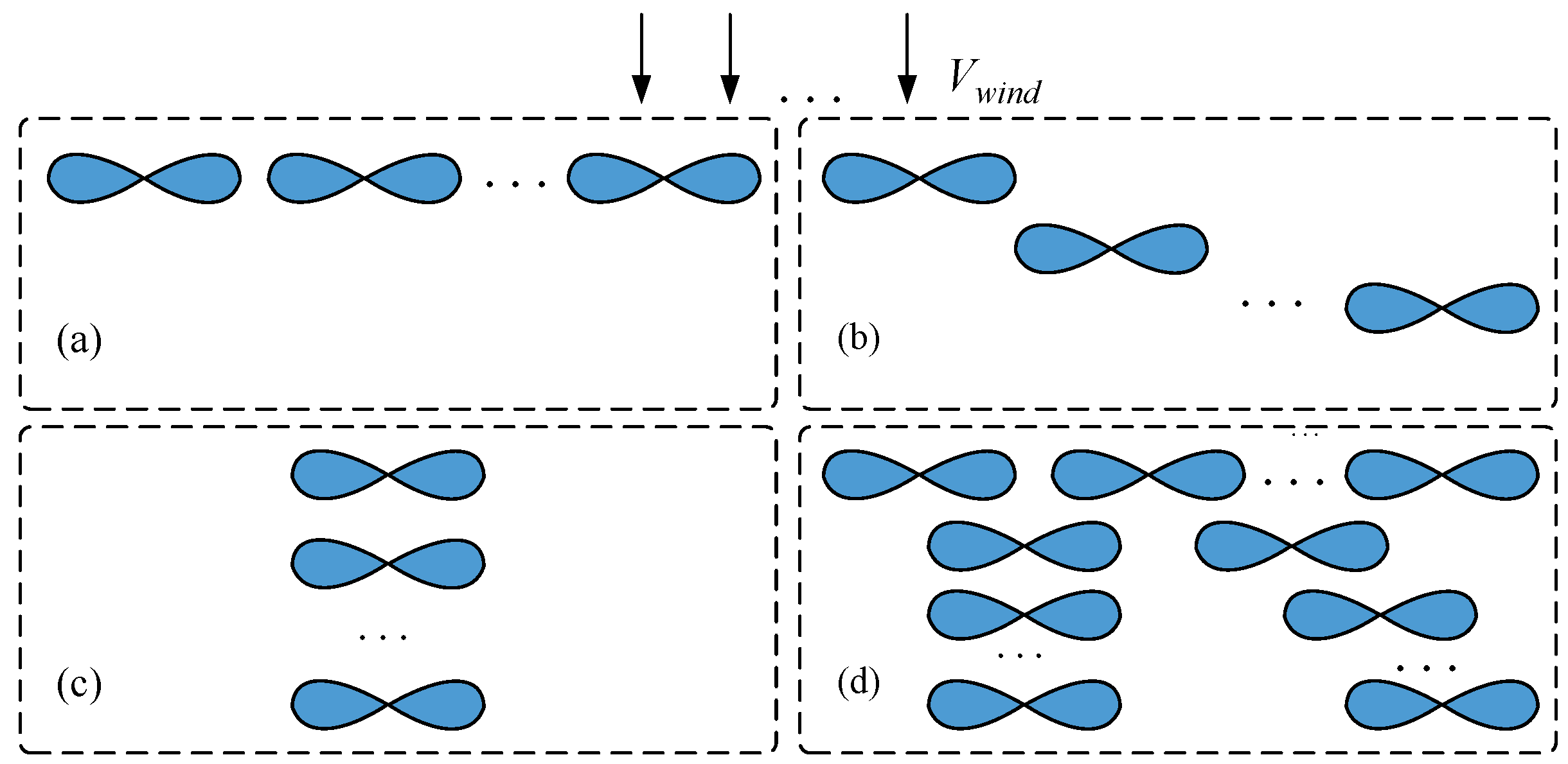
(1) Flat terrain (regular area): Wind farms located offshore, or on non-obstructed flat ground can be considered as regularly on the main wind direction. WTGs are divided into the different clusters according to the types, the capacity, and the position relationship of the wind turbines. The minimum distance between turbines is three to five times the blade diameter within the same row, and five to nine times the blade diameter between rows [56]. The literature [57] has proposed a cluster division method according to the arrangement of wind turbines in wind farms, where wind farms are classified into the horizontal wind farm, vertical wind farm, and the mixed wind farm, as shown in Figure 8.
(2) Complex terrain (irregular area): In practice, the spatial distribution location of WTGs results in different operating states of different turbines. Therefore, “complex terrain” is more in line with wind farms located in hill or mountain areas. The literature [58] has proposed a cluster method based on a constructed diffusion distance measure. First, the power output of each wind turbine is assumed to be a random process with Markovian characteristics; then, the overall process of all the turbines is represented by a Markov transition matrix that is constructed from real data by building a graph with Gaussian weights; finally, the spectral theory is applied to identify the number of clusters and map the original wind turbines to the appropriate cluster. Furthermore, this method has been developed to address the non-linearity and robustness issues in the K-means clustering process, which is a big success in cluster analysis. In [59], a method of probabilistic unit division is proposed. By means of the support vector clustering (SVC) algorithm and according to the historical data of wind speed and direction in one year, the biggest probability of wind speed and direction is used to determine the cluster numbers of wind turbines. The probabilistic clustering requires an initial, one-off, offline analysis of generally available wind farm data (wind measurements at the site, wind farm layout, and electrical parameters of the equipment) to determine the most probable aggregate model of the wind farm, and subsequently leads to a simple aggregate model and short simulation times. However, further study is needed to improve the accuracy of this model, because even the biggest probability is less than 10%. Moreover, the literature has proposed a new algorithm based on fuzzy logic for the wind turbine models [60], and chosen the roots of the mechanical transient characteristic equation for generators as the clustering index for the aggregation modeling of wind farms [61].

3.3.2. Aggregation of Generators

When the types of WTGs are different, or the operating condition differences between the same kinds of wind turbine is large, the generators of WTGs should be respectively aggregated. There are two ideas for the division of wind turbines [8].
(1) Wind turbines with the same or similar operating states have the same or similar transient response characteristics. Therefore, selecting the physical quantities that reflect the operating states is a proper method for turbine division.
(2) The division is carried out according to the types of WTGs, considering transient response characteristics such as the slip homology or the transient voltage characteristic curve [62].
For a large-scale wind farm, the WTGs can be firstly divided into different classes based on their types, and then be divided into different groups based on the operation conditions. Each group of WTGs under similar operation states is aggregated to one WTG. Figure 9 shows the simplified process of the multi-machine aggregation.
The multi-machine aggregated model mainly includes the wind turbine parameters and the generator parameters. To make the distinction, the parameters can be classified into the steady and the transient parameters according to the nature, and these parameters can be subsequently classified according to the sensitivity. The way of parameter aggregation greatly affects the accuracy and validity of the model. At present, there are two kinds of parameter aggregation methods, respectively, the frequency-domain aggregation and the time-domain aggregation. More specifically, the characteristics of these two aggregation methods are:
(1) Frequency-domain aggregation: The frequency characteristics of wind turbines can be fitted effectively. First, the transfer functions of wind turbines are aggregated according to the features of the transfer function of each unit, and then fit to the frequency characteristics of the transfer function, finally obtaining the best fitting point corresponding to the actual response. The least square method can be used for this aggregation method [63,64].
(2) Time-domain aggregation: The aggregation parameters can be adjusted by means of intelligent algorithms such as the genetic algorithm [48] and the neural network algorithm [35], until the aggregation model satisfies the accuracy requirements. The literature [65] has compared several optimization methods, i.e., the basic genetic algorithm, Hopfield neural network, and basic ant colony algorithm, in time complexity, space complexity, and the difficulty of realization by using a paired comparison matrix evaluation method. In this evaluation, the ant colony algorithm has the best performance. However, no single optimization algorithm cannot be considered the best or worst based on one application, as for some applications, one may be better than the others [66].

4. Wind Turbine Generator Transmission Aggregation Model

For a large-scale wind farm, the transmission line and the transformers influence the precision of the aggregation model. Aspects of the WTG transmission system include the layout of wind farms, the size and type of conductors, and the delivery method. The aggregation of the WTG transmission model consists two parts, respectively, the circuit aggregation at the aggregation bus, and the transformer aggregation.
(1) Circuit aggregation: The cable and overhead line are the main types of transmission lines, and are sometimes used together in large-scale wind farms. The cable is relatively unaffected by the environment changes, but the high charging capacitance of the cable may lead to single-phase to ground fault. Overhead lines have a negligible charging capacitor with low voltage and short length. The wire of the overhead line is exposed in the air and is strongly influenced by the environment. When facing severe weather conditions, such as for instance overhead transmission line icing, the safety and reliability are decreased. In a wind farm with hybrid lines, the cables are often constructed in the central region, while the overhead lines are constructed in scattered areas. The cable charging capacitance is 20 to 25 times that of the overhead line, so the susceptance in cables needs to be considered when calculating the equivalent circuit.
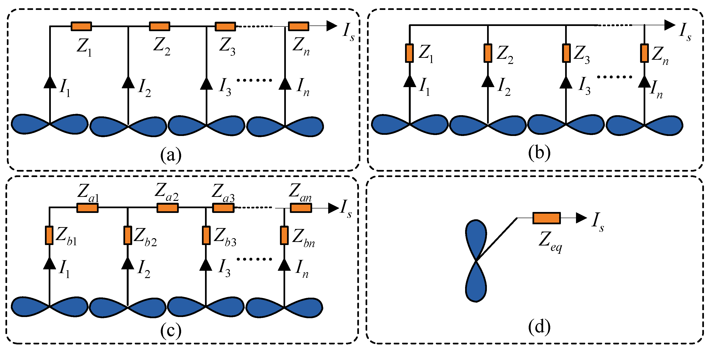
There are three types of connection method that WTGs connect to an aggregation bus: the trunk type, the chain type, and the compound type. Three connection modes of WTGs, and the equivalent aggregation model of the WTG transmission line, are respectively shown in Figure 10.
The aggregation of the trunk type in Figure 10a, Zeq-tr, can be expressed as:
z eq tr = i = 1 n P z i 2 Z i / P z n 2
where Pzi is the total power of Zi.
Similarly, the aggregation of the chain type, Zeq-ch, and the compound type, Zeq-co, are respectively shown in Figure 10b,c, and can be respectively expressed as:
z eq ch = i = 1 n P z i 2 Z i / i = 1 n P z i 2
z eq co = ( i = 1 n n i 2 Z b i + i = 1 n ( j = 1 n n j ) 2 z a i ) / i = 1 n n i 2
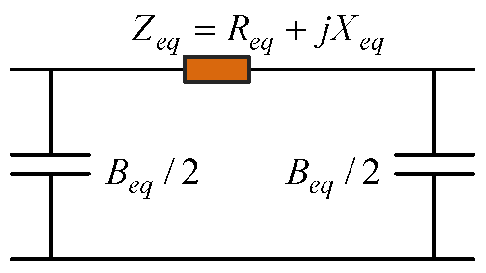
Figure 11 shows the equivalent circuit of the aggregated WTG transmission system. As for the susceptance branch of the cable line, the voltage difference inside the wind farm can be ignored, and the equivalent susceptance equals the sum of all the susceptance of the branches, that is:
B e q = i = 1 m B i
where Bi is the susceptance of the line connected with the i-th wind turbine.
It should be noted that the line loss before and after the equivalence should be equal to each other. Moreover, the objective and working conditions should be considered in the aggregation simplification of WTG transmission topology. The literature [67] has considered the series or parallel relationship of the collector circuits, and proposed an equivalent model based on the parameter transformation. The power aggregation system is usually designed considering the maximum wind power output and the lowest installation and operation cost. The literature [68] has proposed an optimization model for the WTG transmission system of an offshore wind farm that can take different cable cross-sections into account. The literature [69] has also proposed a procedure to optimize the wind turbine location and the line connection topology, by using the genetic algorithm and the ant colony algorithm. The wake effect, the real cable parameters, and the wind speed series are considered when establishing an economical and efficient aggregation model for the offshore wind farm.
(2) Transformer aggregation: Generally, a box transformer substation is adopted to aggregate all of the transformers and keep the voltage drop equal to the sum of all the box transformer substations. The equivalent reactance, Ztrans-eq, can be expressed as follows [70]:
Z t r a n s e q = Z t r a n s / n
where Ztrans is the reactance of one box transformer, and n is the number of the transformers to be aggregated.

5. Conclusions

In this article, a comprehensive survey of aggregation modeling for wind farms was carried out. In wind speed modeling, component models can be used in conjunction with probability distribution models or time-series models when analyzing different characteristics of wind speed. In WTG modeling, a single model delivers satisfactory precision, low computational complexity, and low simulation time when modeling small-scale wind farms. However, when dealing with wind farms consisting of different types of WTGs, or where WTGs work under obvious working condition differences, the single aggregation model may have big errors. The multi-WTG aggregated model should be used in these situations. The aggregation model has high precision when the parameters and working conditions of WTGs in a same aggregation group are close to each other. Meanwhile, when building an aggregation model of a wind farm with large spatial distribution, both circuit aggregation and the transformer aggregation should be considered.
Aggregation modeling is an equivalent simplification for a wind farm, while its legitimate precision is maintained. Based on different aggregation purposes, different division methods of WTGs, simplified hypotheses, and the selection of aggregation types and algorithms can be applied, by which the precision of a wind farm aggregation model is influenced. With more simplified hypotheses and simpler WTG division, the aggregation model will have lower precision, as well as lower computational complexity. Otherwise, the aggregation of a WTG controller under different control strategies and working points is difficult, and the non-linear characteristic of power electronic components may also reduce the precision. Simulations in [71,72,73] showed that when an appropriate aggregation method is chosen, the precision of a wind farm equivalent aggregation model could be as high as 97% of the detailed model, while the complexity is greatly reduced. Meanwhile, the dynamic or transient characteristics of the wind farm for some specific incidents (such as low voltage ride-through behaviors or responses to low-frequency oscillation) are maintained in the aggregation model. Overall, the low complexity and easy application lead to the aggregation models being used more often, compared with detailed models.
Apart from the typical research aforementioned, other techniques in wind farm aggregation modeling should be focused on in the future, such as the methods of actual data selection, the guarantee of the typicality and effectiveness of the collected data, the identification of the important parameters, the prevention of algorithms getting trapped in local optimizations, and the clustering methods considering the large disturbances, the low-frequency oscillations, or the subsynchronous resonance.

Author Contributions

Conceptualization F.L. and M.W.; Writing—Original Draft, F.L. and W.Z.; Writing—Review & Editing, J.M. and F.L.; Investigation J.M. and W.Z.; Supervision, M.W.; Project administration, F.L.

Funding

This research was funded by the Natural Science Foundation of Hunan Province of China grant number 2018JJ2529; by Natural Science Foundation of China grant number 61673398; by the Huxiang Youth Talent Program of Hunan Province grant number 2017RS3006; by NSFC-RFBR Exchange Program grant number 6181101294. The APC was funded by the Natural Science Foundation of Hunan Province of China grant number 2018JJ2529.

Conflicts of Interest

The authors declare no conflict of interest. The funders had no role in the design of the study; in the collection, analyses, or interpretation of data; in the writing of the manuscript, and in the decision to publish the results.

Abbreviations

The following abbreviations are used in this manuscript:
WTGwind turbine generator
AIMSEasymptotic integrated mean squared error
SCIGsquirrel-cage induction generator
DFIGdoubly-fed induction generator
D-PMSGdirect-driven permanent magnet synchronous generator
ARautoregressive
MAmoving average
ARMAautoregressive moving average
ARIMAautoregressive integrated moving average
DSMCdiscrete-state Markov chain
AGCautomatic generation control
PCCpoint of common coupling
SVCsupport vector clustering
SVMsupport vector machine

Appendix A

Table A1. The comparison between the autoregressive integrated moving average (ARMA) model and the discrete state Markov chain model.
Model TypeARMADSMC
Schematic Applsci 09 00769 i001 Applsci 09 00769 i002
Expression x ( k ) = i = 1 n α i x ( k i ) + a ( k ) + j = 1 m β j a ( k j )
where x(k) is the output sequence; a(k) is the zero mean white noise; αi and βj are the autoregressive coefficient and moving average coefficient, respectively; and n and m are autoregressive and moving average order number, respectively.
λ i j = N i j / T i
where Nij and Ti are the number of transitions from state i to j and remaining time in state i, respectively. In the Markov model, the time remaining in each state follows the exponential distribution.
Characteristic
Better autocorrelation features of the original data;
Some negatives produced in simulation cause a certain error in fitting degree of the probability distribution characteristics;
A large number of historical data limits the application.
Keep the probability distribution characteristics and autocorrelation properties of the sample;
Model parameters remain, estimating and selective problems between accuracy and complexity.
Table A2. The four components of the wind speed model.
ComponentDescriptionSchematic
Basic wind (Average wind speed) V A = A Γ ( 1 + 1 / k )
where A is the scale parameter of the Weibull distribution; K is the shape parameter; and Γ is the gamma function.
Applsci 09 00769 i003
Gust wind (Sudden change) V B = { 0 t < t 1 V S t 1 < t < t 1 + T 0 t 1 + T < t , V S = ( V max / 2 ) [ 1 cos ( 2 π × t t 1 T ) ]
where t1 and T are the start time and the period, respectively; and Vmax is the maximum value of the gust wind.
Applsci 09 00769 i004
Gradient wind (Gradual change) V c = { 0 t t 1 V r t 1 < t t 2 V r max t 2 < t , V r = V r max [ 1 ( t 2 t ) / ( t 2 t 1 ) ]
where t1 and t2 are the start time and the terminal time, respectively; and Vr max is the maximum value of the gradient wind.
Applsci 09 00769 i005
Random wind (Random fluctuation) ν w N = 2 i = 1 N [ S V ( ω i ) Δ ω ] cos ( ω i + ϕ i ) , ω i = ( i 1 / 2 ) Δ ω S ν ( ω i ) = 2 K N F 2 | ω i | / π 2 { 1 + [ ( F ω i ) / ( μ π ) ] } 4 / 3
where ϕi are the random variables; and KN, F, μ, N, and ωi are the coefficient of surface roughness, the range of disturbance, the average wind speed of relative height, the number of sampling points, and the frequency of each frequency band, respectively.
Applsci 09 00769 i006
Table A3. Characteristics comparison between the four-component and the two-component model.
ModelFour-Component ModelTwo-Component Model
Complexity ■■
Simulation efficiency■■■■■■
Accuracy
Wind speed curve always has a big change.
Without constraint over the probability distribution and frequency change of wind speed, the generated wind speed sequence is quite different from reality.
The wind speed curve clearly shows the differences between the high-frequency and low-frequency components.
Applicability
Given no calculation method of gust component parameters, it can only simulate simple situations.
A narrow range of wind speed could be covered.
Cannot reflect the various trend of wind speed changes.
Legenda: ■—Small; ■■—Medium; ■■■—Strong.

References

  1. Global Wind Energy Outlook 2014. Available online: http://www.gwec.net/wp-content/uploads/2014/10/GWEO2014_WEB.pdf (accessed on 21 October 2014).
  2. Steve, S.; Klaus, R.; Kenneth, H. Global Wind Report Annual Market Update 2017. Available online: http://files.gwec.net/register?file=/files/GWR2017.pdf (accessed on 25 April 2018).
  3. Mahmoud, T.; Dong, Z.; Ma, J. An advanced approach for optimal wind power generation prediction intervals by using self-adaptive evolutionary extreme learning machine. Renew. Energy 2018, 126, 254–269. [Google Scholar] [CrossRef]
  4. Bu, S.; Zhang, X.; Zhu, J.; Liu, X. Comparison analysis on damping mechanisms of power systems with induction generator based wind power generation. Int. J. Electr. Power Energy Syst. 2018, 97, 250–261. [Google Scholar] [CrossRef]
  5. Hsu, C.T.; Korimara, R.; Cheng, T. Power quality analysis for the distribution systems with a wind power generation system. Comput. Electr. Eng. 2016, 54, 131–136. [Google Scholar] [CrossRef]
  6. Meng, W.; Wang, X. Distributed Energy Management in Smart Grid with Wind Power and Temporally Coupled Constraints. IEEE Trans. Ind. Electron. 2017, 64, 6052–6062. [Google Scholar] [CrossRef]
  7. Yang, H.; Pan, H.; Luo, F.; Qiu, J. Operational Planning of Electric Vehicles for Balancing Wind Power and Load Fluctuations in a Microgrid. IEEE Trans. Sustain. Energy 2017, 8, 592–604. [Google Scholar] [CrossRef]
  8. Ding, M.; Zhu, Q.; Han, P. Wind farm equivalent modeling research. Smart Grid 2014, 2, 1–6. [Google Scholar]
  9. Sun, S.; Liu, F.; Xue, S. Review on wind power development in China: Current situation and improvement strategies to realize future development. Renew. Sustain. Energy Rev. 2015, 45, 589–599. [Google Scholar] [CrossRef]
  10. Thomas, E.; Patrik, S. Wind power, regional development and benefit-sharing: The case of Northern Sweden. Renew. Sustain. Energy Rev. 2015, 47, 476–485. [Google Scholar]
  11. Aigner, T.; Jaehnert, S.; Doorman, G.L. The Effect of Large-Scale Wind Power on System Balancing in Northern Europe. Sustain. Energy 2012, 3, 751–759. [Google Scholar] [CrossRef]
  12. Li, Y.; He, L.; Liu, F.; Tan, Y.; Cao, Y.; Luo, L.; Shahidehpour, M. A dynamic coordinated control strategy of WTG-ES combined system for short-term frequency support. Renew. Energy 2018, 119, 1–11. [Google Scholar]
  13. Gala-Santos, M.L. Aerodynamic and Wind Field Models for wind Turbine Control. Ph.D. Thesis, University of Strathclyde, Glasgow, UK, 2016. [Google Scholar]
  14. Hur, S.; Leithead, W.E. Adjustment of wind farm power output through flexible turbine operation using wind farm control. Wind Energy 2016, 19, 1667–1686. [Google Scholar] [CrossRef]
  15. Hur, S. Modelling and control of a wind turbine and farm. Energy 2018, 156, 360–370. [Google Scholar] [CrossRef]
  16. Miao, S.; Xie, K.; Yang, H.; Tai, H.; Hu, B. Markovian wind farm generation model and its application to adequacy assessment. Renew. Energy 2017, 113, 1447–1461. [Google Scholar] [CrossRef]
  17. Dobakhshari, A.S.; Fotuhi-Firuzabad, M. A reliability model of large wind farms for power system adequacy studies. IEEE Trans. Energy Convers. 2009, 24, 792–801. [Google Scholar] [CrossRef]
  18. Ghaedi, A.; Abbaspour, A.; Fotuhi-Firuzabad, M. Toward a comprehensive model of large-scale DFIG-based wind farms in adequacy assessment of power systems. IEEE Trans. Sustain. Energy 2014, 5, 55–63. [Google Scholar] [CrossRef]
  19. Chandra, D.R.; Kumari, M.S.; Sydulu, M.; Grimaccia, F.; Mussetta, M.; Leva, S.; Duong, M.Q. Small signal stability of power system with SCIG, DFIG wind turbines. In Proceedings of the IEEE India Conference, Pune, India, 11–13 December 2014. [Google Scholar]
  20. Cao, N.; Zhao, H.; Chen, M.; Dai, H. Equivalence Method of Wind Farm in Steady-State Load Flow Calculation. Power Syst. Technol. 2006, 30, 53–56. [Google Scholar]
  21. Zou, J.; Peng, C.; Yan, Y. A survey of dynamic equivalent modeling for wind farm. Renew. Sustain. Energy Rev. 2014, 40, 956–963. [Google Scholar] [CrossRef]
  22. Hussein, D.N.; Matar, M.; Iravani, R. A Type-4 Wind Power Plant Equivalent Model for the Analysis of Electromagnetic Transients in Power Systems. IEEE Trans. Power Syst. 2013, 28, 3096–3104. [Google Scholar] [CrossRef]
  23. Chellali, F.; Khellaf, A.; Belouchrani, A.; Khanniche, R. A comparison between wind speed distributions derived from the maximum entropy principle and Weibull distribution Case of study; six regions of Algeria. Renew. Sustain. Energy Rev. 2012, 1, 379–385. [Google Scholar] [CrossRef]
  24. Yao, F.; Zhao, Y.; Meng, K. Quantum-Inspired Particle Swarm Optimization for Power System Operations Considering Wind Power Uncertainty and Carbon Tax in Australia. IEEE Trans. Ind. Inform. 2012, 4, 880–888. [Google Scholar] [CrossRef]
  25. Qin, Z.; Li, W.; Xiong, X. Estimating wind speed probability distribution using kernel density method. Electric Power Syst. Res. 2011, 81, 2139–2146. [Google Scholar] [CrossRef]
  26. Zhang, Y.; Wang, J.; Wang, X. Review on probabilistic forecasting of wind power generation. Renew. Sustain. Energy Rev. 2014, 32, 255–270. [Google Scholar] [CrossRef]
  27. Miao, S.; Xie, K.; Yang, H.; Karki, R.; Tai, H.M.; Chen, T. A mixture kernel density model for wind speed probability distribution estimation. Energy Convers. Manag. 2016, 126, 1066–1083. [Google Scholar] [CrossRef]
  28. Wangdee, W.; Billinton, R. Considering load-carrying capability and wind speed correlation of WECS in generation adequacy assessment. IEEE Trans. Energy Convers. 2006, 3, 734–741. [Google Scholar] [CrossRef]
  29. Liu, X. Economic Load Dispatch Constrained by Wind Power Availability: A Wait-and-See Approach. IEEE Trans. Smart Grid 2010, 1, 347–355. [Google Scholar] [CrossRef]
  30. Xu, D.; Gao, F.; Lv, Y. Modeling and simulation of wind speed on wind farm by applying higher-order statistics. J. North China Electric Power Univ. 2008, 3, 12–16. [Google Scholar]
  31. Liu, H.; Shi, J.; Qu, X. Empirical investigation on using wind speed volatility to estimate the operation probability and power output of wind turbines. Energy Convers. Manag. 2013, 67, 8–17. [Google Scholar] [CrossRef]
  32. Han, X.; Qu, Y.; Wang, P. Four-Dimensional Wind Speed Model for Adequacy Assessment of Power Systems with Wind Farms. IEEE Trans. Power Syst. 2012, 3, 2978–2985. [Google Scholar] [CrossRef]
  33. Hoolohan, V.; Tomlin, A.S.; Cockerill, T. Improved near surface wind speed predictions using Gaussian process regression combined with numerical weather predictions and observed meteorological data. Renew. Energy 2018, 126, 1043–1054. [Google Scholar] [CrossRef]
  34. Yu, C.; Li, Y.; Bao, Y.; Tang, H.; Zhai, G. A novel framework for wind speed prediction based on recurrent neural networks and support vector machine. Energy Convers. Manag. 2018, 178, 137–145. [Google Scholar] [CrossRef]
  35. Xiao, Q.; Cong, J.; Wang, J. Online Clustering for Wind Speed Forecasting Based on Combination of RBF Neural Network and Persistence Method. In Proceedings of the Chinese Control and Decision Conference (CCDC), Mianyang, China, 23–25 May 2011. [Google Scholar]
  36. Duong, M.Q.; Grimaccia, F.; Leva, S.; Mussetta, M.; Sava, G.; Costinas, S. Performance analysis of grid-connected wind turbines. Sci. Bull. Politehn. Univ. Buchar. Ser. C Electr. Eng. Comput. Sci. 2014, 76, 169–180. [Google Scholar]
  37. Rodrıguez-Amenedo, J.L.; Arnaltes, S.; Rodrıguez, M.A. Operation and coordinated control of fixed and variable speed wind farms. Renew. Energy 2008, 33, 406–414. [Google Scholar] [CrossRef]
  38. Mi, Z.; Su, X.; Yang, Q. Multi-Machine Representation Method for Dynamic Equivalent Model of Wind Farms. Trans. China Electrotech. Soc. 2010, 25, 162–169. [Google Scholar]
  39. Peak. The dynamic equivalence of D-PMSG wind turbine based wind farms. Power Syst. Technol. 2012, 36, 222–227. [Google Scholar]
  40. Xia, Y.; Li, Z.; Cai, X.; Ma, Y. Dynamic Modeling of Wind Farm Composed of Direct-Driven Permanent Magnet Synchronous Generators. Power Syst. Technol. 2014, 38, 1439–1445. [Google Scholar]
  41. Luis, M.; Fernandez, J.R.; Saenz, F.J. Dynamic models of wind farms with fixed speed wind turbines. Renew. Energy 2006, 31, 1203–1230. [Google Scholar]
  42. Kim, H.; Singh, C.; Sprintson, A. Simulation and Estimation of Reliability in a Wind Farm Considering the Wake Effect. IEEE Trans. Sustain. Energy 2011, 3, 274–282. [Google Scholar] [CrossRef]
  43. Hou, G.; Zheng, X.; Jiang, P. Study of Modeling and Intelligent Control on AGC System with Wind Power. In Proceedings of the Control and Decision Conference (CCDC), Changsha, China, 31 May–2 June 2014. [Google Scholar]
  44. Gao, F.; Zhao, D.; Zhou, X. Dynamic Equivalent Algorithm for Wind Farm Composed of Direct-Drive Wind Turbines. Power Syst. Technol. 2012, 36, 222–227. [Google Scholar]
  45. Perdana, A.; Uski, J.S.; Carlson, O. Comparison of an aggregated model of a wind farm consisting of fixed-speed wind turbines with field measurement. Wind Energy 2008, 11, 13–27. [Google Scholar] [CrossRef] [Green Version]
  46. Chien, L.C.; Sun, C.C.; Yeh, Y.J. Modeling of Wind Farm Participation in AGC. IEEE Trans. Power Syst. 2013, 3, 1204–1211. [Google Scholar] [CrossRef]
  47. Wang, H. Research on Equivalent Modelling of Wind Farms and Transient Operational Performances; College of Electrical Engineering of Chongqing University: Chongqing, China, 2010. [Google Scholar]
  48. Li, H.; Yang, C.; Zhao, B.; Wang, H.; Chen, Z. Aggregated models and transient performances of a mixed wind farm with different wind turbine generator systems. Electric Power Syst. Res. 2012, 92, 1–10. [Google Scholar] [CrossRef]
  49. Chavez-Baez, M.V.; Anaya-Lara, O.; Lo, K.L.; McDonald, J. Harmonics and power loss reduction in multi-technology offshore wind farms using simplex method. In Proceedings of the Power Engineering Conference (UPEC), Dublin, Ireland, 2–5 September 2013. [Google Scholar]
  50. Opathella, C.; Cheng, D.; Venkatesh, B. An intelligent wind farm model for three-phase unbalanced power flow studies. In Proceedings of the Engineering Technology and Technopreneuship (ICE2T), Kuala Lumpur, Malaysia, 27–29 August 2014. [Google Scholar]
  51. Li, Y.; He, L.; Liu, F.; Li, C.; Cao, Y.; Shahidehpour, M. Flexible Voltage Control Strategy Considering Distributed Energy Storages for DC Distribution Network. IEEE Trans. Smart Grid 2018, 10, 163–172. [Google Scholar] [CrossRef]
  52. Fernández, L.M.; Jurado, F.; Saenz, J.R. Aggregated dynamic model for wind farms with doubly fed induction generator wind turbines. Renew. Energy 2008, 33, 129–140. [Google Scholar] [CrossRef]
  53. Aoller, M.P.; Achilles, S. Aggregated wind park models for analyzing power system dynamics. In Proceedings of the International Workshop on Large Scale Integration of Wind Power and Transmission Networks for Offshore Wind Farms, Billund, Denmark, 20–21 October 2003. [Google Scholar]
  54. Han, X.; Guo, J.; Wang, P. Adequacy study of a wind farm considering terrain and wake effect. IET Gener. Transm. Distrib. 2012, 6, 1001–1008. [Google Scholar] [CrossRef]
  55. Kuenzel, S.; Kunjumuhammed, L.P.; Pal, B.C.; Erlich, I. Impact of Wakes on Wind Farm Inertial Response. IEEE Trans. Sustain. Energy 2014, 5, 237–245. [Google Scholar] [CrossRef]
  56. Muljadi, E.; Nguyen, T.B.; Pai, M.A. Impact of Wind Power Plants on Voltage and Transient Stability of Power Systems. In Proceedings of the Energy 2030 Conference, Atlanta, GA, USA, 17–18 November 2008. [Google Scholar]
  57. Banakar, H.; Teckooi, B. Clustering of Wind Farms and its Sizing Impact. IEEE Trans. Energy Convers. 2009, 24, 935–942. [Google Scholar] [CrossRef]
  58. Ma, Y.; Runolfsson, T.; Jiang, J. Cluster analysis of wind turbines of large wind farm with diffusion distance method. IET Renew. Power Gener. 2011, 5, 109–116. [Google Scholar] [CrossRef]
  59. Ali, M. Wind Farm Model Aggregation Using Probabilistic Clustering. IEEE Trans. Power Syst. 2013, 28, 309–316. [Google Scholar] [CrossRef]
  60. Taner, U.; Ahmet, D.Ş. Wind turbine power curve estimation based on cluster center fuzzy logic modeling. J. Wind Eng. Ind. Aerodyn. 2008, 96, 611–620. [Google Scholar]
  61. Yan, G. Discussion on the equivalent values of DFIG included wind farm. Renew. Energy Resour. 2008, 26, 21–23. [Google Scholar]
  62. Zhang, B.; Zhang, Y.; Zhong, Q.; Du, Z. Application of Dynamic Equivalence Based on Coherency in South China Power Grid. In Proceedings of the Asia-Pacific Power and Energy Engineering Conference, Wuhan, China, 25–28 March 2011. [Google Scholar]
  63. Thapar, V.; Agnihotri, G.; Vinod, K.S. Critical analysis of methods for mathematical modelling of wind turbines. Renew. Energy 2011, 36, 3166–3177. [Google Scholar] [CrossRef]
  64. Yampikulsakul, N.; Eunshin, B.; Huang, S.; Shuang, W.S. Condition Monitoring of Wind Power System with Nonparametric Regression Analysis. IEEE Trans. Energy Convers. 2014, 29, 288–299. [Google Scholar]
  65. Wang, H. Comparison of several intelligent algorithms for solving TSP problem in industrial engineering. Syst. Eng. Procedia 2012, 4, 226–235. [Google Scholar] [Green Version]
  66. Sasmita, B.; Subhrajit, S.; Patib, B.B. A review on optimization algorithms and application to wind energy integration to grid. Renew. Sustain. Energy Rev. 2015, 48, 214–227. [Google Scholar]
  67. Abuaisha, T.S. General study of the control principles and dynamic fault behaviour of variable-speed wind turbine and wind farm generic models. Renew. Energy 2014, 68, 245–254. [Google Scholar] [CrossRef]
  68. Francisco, M.; Longatt, G.; Peter, W.; Pawel, R.; Vladimir, T. Optimal Electric Network Design for a Large Offshore Wind Farm Based on a Modified Genetic Algorithm Approach. IEEE Syst. J. 2012, 6, 164–172. [Google Scholar]
  69. Wu, Y.K.; Lee, C.Y.; Chen, C.R.; Hsu, K.W.; Tseng, H.T. Optimization of the Wind Turbine Layout and Transmission System Planning for a Large-Scale Offshore Wind Farm by AI Technology. IEEE Trans. Ind. Appl. 2014, 50, 2071–2080. [Google Scholar] [CrossRef]
  70. Muljadi, E. Equivalencing the collector system of a large wind power plant. In Proceedings of the IEEE Power Engineering Society General Meeting, Montreal, QC, Canada, 18–22 June 2006. [Google Scholar]
  71. Chowdhury, M.A.; Hosseinzadeh, N.; Billah, M.M.; Haque, S.A. Dynamic DFIG wind farm model with an aggregation technique. In Proceedings of the International Conference on Electrical & Computer Engineering, Dhaka, Bangladesh, 18–20 December 2011. [Google Scholar]
  72. Zhang, M.; Li, Q.; Liu, C.; Zhang, J. An aggregation modeling method of large-scale wind farms in power system transient stability analysis. In Proceedings of the International Conference on Power System Technology, Guangzhou, China, 6–8 November 2018. [Google Scholar]
  73. Ruan, J.; Lu, Z.G.; Qiao, Y.; Min, Y. Analysis on applicability problems of the aggregation-based representation of wind farms considering DFIGs’ LVRT behaviors. IEEE Trans. Power Syst. 2016, 31, 4953–4965. [Google Scholar] [CrossRef]
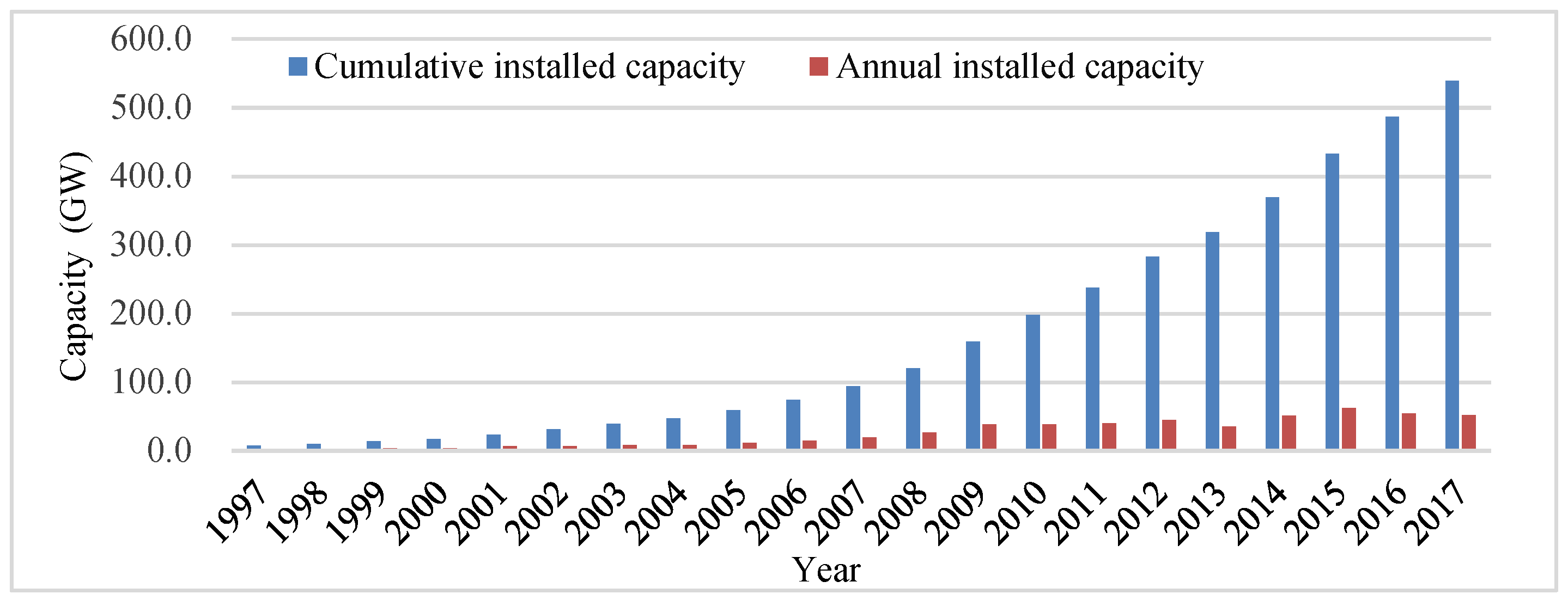
Figure 1. The global installed capacity of wind power during 1997–2017.
Applsci 09 00769 g001
Figure 2. The top 10 global countries for total wind power capacity in 2017.
Applsci 09 00769 g002
Figure 3. Wind power capacity from 2017 to 2022.
Applsci 09 00769 g003
Figure 4. The framework of the wind farm modeling with the aggregating method.
Applsci 09 00769 g004
Figure 5. The structures of three different types of wind turbines: (a) the squirrel-cage asynchronous wind turbine; (b) the double-fed induction wind turbine; and (c) the direct-drive permanent magnet synchronous wind turbine.
Applsci 09 00769 g005aApplsci 09 00769 g005b
Figure 6. The aggregation of the “single wind turbine + single generator” model.
Applsci 09 00769 g006
Figure 7. The aggregation process with the aggregation of different wind turbines.
Applsci 09 00769 g007
Figure 8. The different arrangement of wind turbines, (a) the horizontal wind farm; (b) the vertical–diagonal wind farm; (c) the vertical–longitudinal wind farm; and (d) the mixed wind farm.
Applsci 09 00769 g008
Figure 9. Multi-machine aggregation method.
Applsci 09 00769 g009
Figure 10. Connection types of wind turbines: (a) the trunk type; (b) the chain type; (c) the compound type; and (d) the aggregation of different connection types.
Applsci 09 00769 g010
Figure 11. The equivalent circuit of the aggregated wind turbine generator (WTG) transmission system.
Applsci 09 00769 g011