Intelligent Evaluation of Strabismus in Videos Based on an Automated Cover Test

Abstract

Strabismus is a common vision disease that brings about unpleasant influence on vision, as well as life quality. A timely diagnosis is crucial for the proper treatment of strabismus. In contrast to manual evaluation, well-designed automatic evaluation can significantly improve the objectivity, reliability, and efficiency of strabismus diagnosis. In this study, we have proposed an innovative intelligent evaluation system of strabismus in digital videos, based on the cover test. In particular, the video is recorded using an infrared camera, while the subject performs automated cover tests. The video is then fed into the proposed algorithm that consists of six stages: (1) eye region extraction, (2) iris boundary detection, (3) key frame detection, (4) pupil localization, (5) deviation calculation, and (6) evaluation of strabismus. A database containing cover test data of both strabismic subjects and normal subjects was established for experiments. Experimental results demonstrate that the deviation of strabismus can be well-evaluated by our proposed method. The accuracy was over 91%, in the horizontal direction, with an error of 8 diopters; and it was over 86% in the vertical direction, with an error of 4 diopters.

1. Introduction

Strabismus is the misalignment of the eyes, that is, one or both eyes may turn inward, outward, upward, or downward. It is a common ophthalmic disease with an estimated prevalence of 4%, in adulthood [1], 65% of which develops in childhood [2]. Strabismus could have serious consequences on vision, especially for children [3,4]. When the eyes are misaligned, the eyes look in different directions, leading to the perception of two images of the same object, a condition called diplopia. If strabismus is left untreated in childhood, the brain eventually suppresses or ignores the image of the weaker eye, resulting in amblyopia or permanent vision loss. Longstanding eye misalignment might also impair the development of depth perception or the ability to see in 3D. In addition, patients with paralytic strabismus might turn their face or head to overcome the discomfort and preserve the binocular vision for the paralyzed extraocular muscle, which might lead to a skeletal deformity in children, such as scoliosis. More importantly, it has been shown that people with strabismus show higher levels of anxiety and depression [5,6] and report a low self-image, self-esteem, and self-confidence [7,8], which brings adverse impact on a person’s life, including education, employment, and social communication [9,10,11,12,13,14]. Thus, timely quantitative evaluation of strabismus is essential, in order to get a suitable treatment for strabismus. More specifically, accurate measurement of the deviation in strabismus is crucial in planning surgery and other treatments.

Currently, several tests need to be performed, usually, to diagnose strabismus in a clinical context [15]. For example, the corneal light reflex is conducted by directly observing the displacement of the reflected image of light from the center of the pupil. Maddox rod is a technique that utilizes filters and distorting lenses for quantifying eye turns. Another way to detect and measure an eye turn is to conduct a cover test, which is the most commonly used technique. All these methods require conduction and interpretation by the clinician or ophthalmologist, which is subjective to some extent. Taking the cover test as an example, the cover procedures and assessments are conducted manually, in the existing clinical systems, and well-trained specialists are needed for the test. Therefore, this limits the effect of strabismus assessment in two aspects [16,17]. With respect to cover procedure, the cover is given manually, so the covering time and speed of occluder movement depend on the experience of the examiners and can change from time to time. These variations of the cover may influence the assessment results. With respect to assessment, the response of subject is evaluated subjectively, which leads to more uncertainties and limitations in the final assessment. First, the direction of eye movement, the decision of whether or not moving and the responding speed for recovery, rely on the observation and determination of the examiners. The variances of assessment results, among examiners, cannot be avoided. Second, the strabismus angle has to be measured with the aid of a prism, in a separate step and by trial-and-error. This strings out the diagnosis process. Being aware of these clinical disadvantages, researchers are trying to find novel ways to improve the process of strabismus assessment.

With the development of computer technology, image acquisition technology, etc., researchers have made some efforts to utilize new technologies and resources to aid ophthalmology diagnostics. Here, we give a brief review on the tools and methodologies that support the detection and diagnosis of strabismus. These methods can be summarized into two categories, namely the image-based or video-based method, and the eye-tracking based method.

The image-based or video-based method uses image processing techniques to achieve success in diagnosing strabismus [18,19,20,21,22]. Helveston [18] proposed a store-and-forward telemedicine consultation technique that uses a digital camera and a computer to obtain patient images and then transmits them by email, so the diagnosis and treatment plan could be determined by the experts, according to the images. This was an early attempt to apply new resources to aid the diagnosis of strabismus. Yang [19] presented a computerized method of measuring binocular alignment, using a selective wavelength filter and an infrared camera. Automated image analysis showed an excellent agreement with the traditional PCT (prism and alternate cover test). However, the subjects who had an extreme proportion that fell out of the normal variation range, could not be examined using this system, because of its software limitations. Then in [20], they implemented an automatic strabismus examination system that used an infrared camera and liquid crystal shutter glasses to simulate a cover test and a digital video camera, to detect the deviation of eyes. Almedia et al. [21] proposed a four-stage methodology for automatic detection of strabismus in digital images, through the Hirschberg test: (1) finding the region of the eyes; (2) determining the precise location of eyes; (3) locating the limbus and the brightness; and (4) identifying strabismus. Finally, it achieved a 94% accuracy in classifying individuals with or without strabismus. However, the Hirschberg test was less precise compared to other methods like the cover test. Then in [22], Almeida presented a computational methodology to automatically diagnose strabismus through digital videos featuring a cover test, using only a workstation computer to process these videos. This method was recognized to diagnose strabismus with an accuracy value of 87%. However, the effectiveness of the method was considered only for the horizontal strabismus and it could not distinguish between the manifest strabismus and the latent strabismus.

The eye-tracking technique was also applied for strabismus examination [23,24,25,26,27]. Quick and Boothe [23] presented a photographic method, based on corneal light reflection for the measurement of binocular misalignment, which allowed for the measurement of eye alignment errors to fixation targets presented at any distance, throughout the subject’s field of gaze. Model and Eizenman [24] built up a remote two-camera gaze-estimation system for the AHT (Automated Hirschberg Test) to measure binocular misalignment. However, the accuracy of the AHT procedure has to be verified with a larger sample of subjects, as it was studied on only five healthy infants. In [25], Pulido proposed a new method prototype to study the eye movement where gaze data were collected using the Tobii eye tracker, to conduct ophthalmic examination, including strabismus, by calculating the angles of deviation. However, the thesis focused on the development of the new method to provide repeatability, objectivity, comprehension, relevance, and independence and lacked an evaluation of patients. In [26], Chen et al. developed an eye-tracking-aided digital system for strabismus diagnosis. The subject’s eye alignment condition was effectively investigated by intuitively analyzing gaze deviations, but only a strabismic person and a normal person were asked to participate in the experiments. Later, in [27], Chen et al developed a more effective eye-tracking system to acquire gaze data for strabismus recognition. Particularly, they proposed a gaze deviation image to characterize eye-tracking data and then leveraged the Convolutional Neural Networks to generate features from gaze deviation image, which finally led to an effective strabismus recognition. However, the performance of the proposed method could be further evaluated with more gaze data, especially data with different strabismus types.

In this study, we have proposed an intelligent evaluation system for strabismus. Intelligent evaluation of strabismus, which could also be termed an automatic strabismus assessment, assesses strabismus without ophthalmologists. We developed a set of intelligent evaluation systems in digital videos based on a cover test, in which an automatic stimulus module, controlled by chips, was used to generate the cover action of the occluder; the synchronous tracking module was used to monitor and record the movement of eyes; and the algorithm module was used to analyze the data and generate the measurement results of strabismus.

The rest of paper is organized as follows. A brief introduction of the system is given in Section 2. The methodology exploited for strabismus evaluation is described in detail in Section 3. Then, in Section 4, the results achieved by our methodology are presented, and in Section 5, some conclusions are drawn and a prospect of future work is discussed.

2. System Introduction

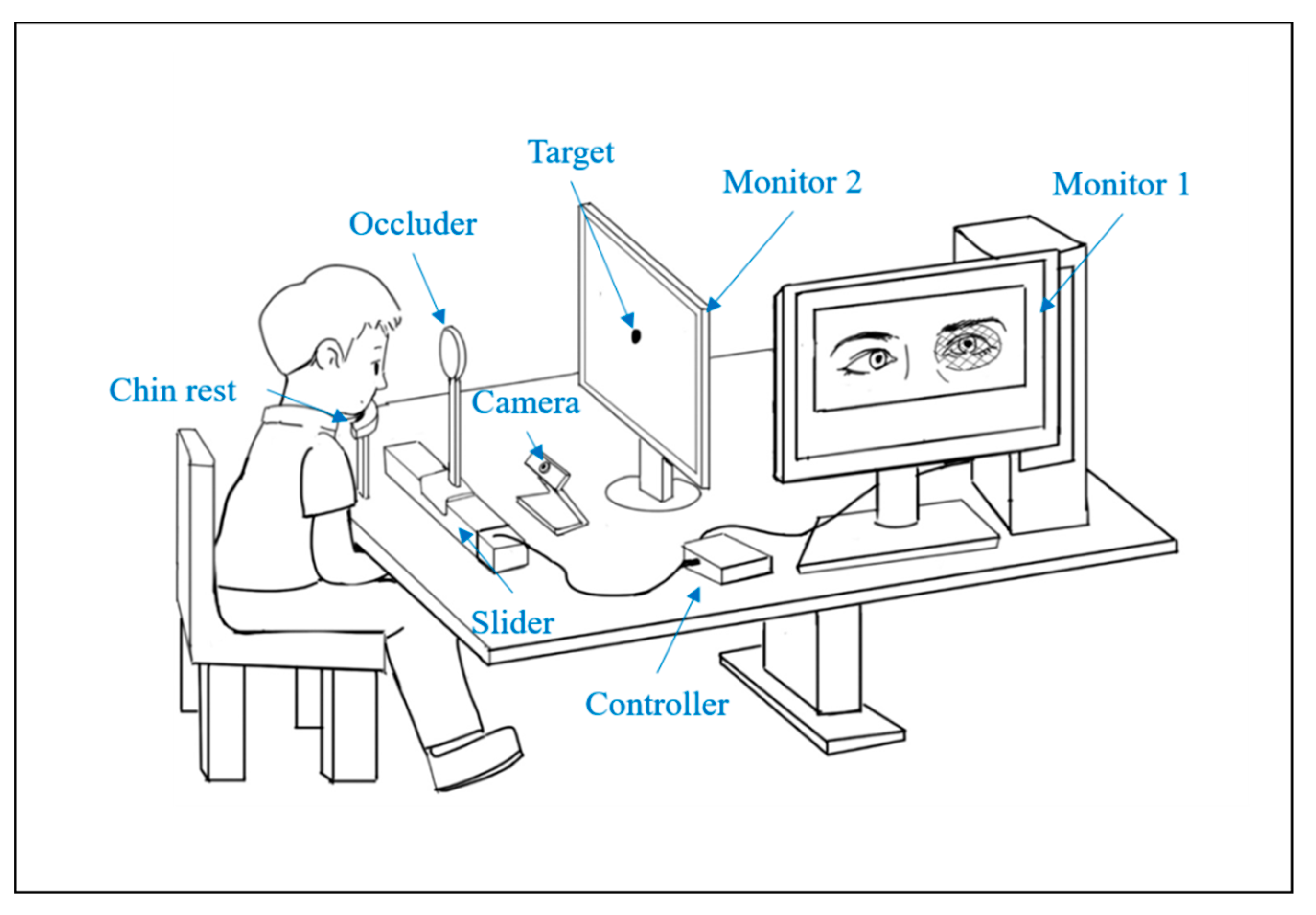
In our work, we have developed a set of intelligent evaluation systems of strabismus, in which the subject needs to sit on the chair with his chin on the chin rest and fixate on the target. The cover tests are automatically performed and finally a diagnosis report is generated, after a short while. The system, as shown in Figure 1, can be divided into three parts, i.e., the automated stimulus module for realizing the cover test, the video acquisition module for motion capture, and the algorithm module for detection and measurement of strabismus. More details of the system have been presented in our previous work [28].

2.1. Hardware Design

The automated stimulus module is based on a stepper motor connected to the controller, a control circuit, which makes the clinical cover test automated. The stepper motor used in the proposed system is iHSV57-30-10-36, produced by JUST MOTION CONTROL (Shenzhen, China). The occluder is hand-made cardboard, 65 mm wide, 300 mm high, and 5 mm thick. The subject’s sight is completely blocked when the occluder occludes the eye so that our method can properly simulate the clinical cover test. XC7Z020, a Field Programmable Gate Array (FPGA), is the core of the control circuit. The communication between the upper computer and the FPGA is via a Universal Serial Bus (USB). The motor rotates at a particular speed in a particular direction, clockwise or counterclockwise, to drive the left and right movement of the occluder on the slider, once the servo system receives the control signals from the FPGA.

As for the motion-capture module, the whole process of the test is acquired by the high-speed camera RER-USBFHD05MT with a $1280\times 720$ resolution at 60 fps. A near-infrared led array with a spectrum of 850 nm and a near-infrared lens were selected to compensate for the infrared light illumination and separately reduce the noise from the visible light. AMCap is used to perform the control of the camera, such as the configuration of the frame rate and resolution, exposure time, the start and end of a recording, and so on.

Being ready to execute the strabismus evaluation, the subject is told to sit in front of the workbench with chin on the chin rest and fixate on the given target. The target is a cartoon character displayed on a MATLAB GUI on Monitor 2, for the purpose of attracting attention, especially for children. The experimenter sends a code “0h07” (the specific code for automatic cover test) to the system, and the stimulus module reacts to begin the process of the cover test. Meanwhile, the video acquisition application AMCap automatically starts recording. When the cover test ends, AMCap stops recording and saves the video in a predefined directory. Then the video is fed into the proposed intelligent algorithm performing the strabismus evaluation. Finally, a report is generated automatically which contains the presence, type, and degree of strabismus.

2.2. Data Collection

In the cover test, the examiner covers one of the subject’s eyes and uncovers it, repeatedly, to see whether the non-occluded eye moves or not. If the movement of the uncovered eye can be observed, the subject is thought to have strabismus. The cover test can be divided into three subtypes—the unilateral cover test, the alternating cover test, and the prism alternate cover test. The unilateral cover test is used principally to reveal the presence of a strabismic deviation. If the occlusion time is extended, it is also called the cover-uncover test [29]. The alternating cover test is used to quantify the deviation [30]. The prism alternate cover test is known as the gold standard test to obtain the angle of ocular misalignment [31]. In our proposed system, we sequentially performed the unilateral cover test, the alternate cover test, and the cover-uncover test, for each subject, to check the reliability of the assessment.

The protocol of the cover tests is as follows. Once the operator sends out the code “0h07”, the automatic stimulus module waits for 6 s to let the application “AMCap” react, and then the occlusion operation begins. The occluder is initially held in front of the left eye. The first is the unilateral cover test for the left eye—the occluder moves away from the left eye, waiting for 1 s, then moves back to cover the left eye for 1 s. This process is repeated for three times. The unilateral cover test for the right eye is the same as that of the left eye. When this procedure ends, the occluder is at the position of occluding the right eye. Then the alternate cover test begins. The occluder moves to the left to cover the left eye for 1 s and then moves to the right to cover the right eye. This is considered as one round, and it needs to be repeated for three rounds. Finally, the cover-uncover test is performed for both eyes. The only difference from the above unilateral cover test is that the time of the occluder’s occluding eyes is increased to 2 s. Eventually, the occluder returns to the initial position.

We cooperated with the Hong Kong Association of Squint and Double Vision Sufferers to collect strabismic data. In total 15 members of the association consented to participate in our experiments. In addition to the 15 adult subjects, 4 children were invited to join our study. The adults and children, including both male and female, were within the age ranges of 25 to 63 years and 7 to 10 years, respectively. The camera was configured to capture a resolution of $1280\times 720$ pixels at a frame rate of 60 fps. The distance between the target and eyes was 33 cm. If wearing corrective lenses, the subject was requested to perform the tests twice, once wearing it and once without it. After ethics approval and informed consent, the 19 subjects followed the data acquisition procedure introduced above, to participate in the experiments. Finally, 24 samples were collected, five of which were with glasses.

3. Methodology

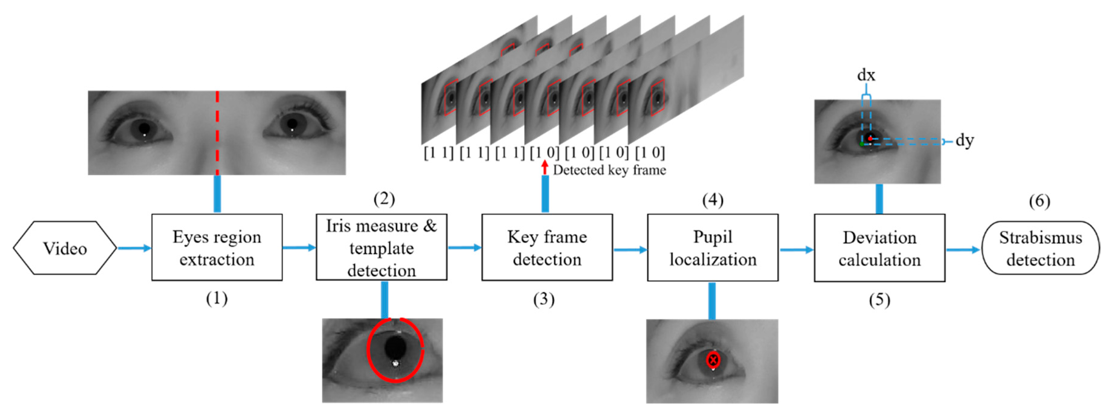
To assess the strabismus, it is necessary to determine the extent of unconscious movement of eyes when applying the cover test. To meet the requirement, a method consisting of six stages is proposed, as shown in Figure 2. (1) The video data are first processed to extract the eye regions, to get ready for the following procedures. (2) The iris measure and template is detected to obtain its size for the further calculations and segment region for the template matching. (3) The key frame is detected to locate the position at which the stimuli occur. (4) The pupil localization is performed to identify the coordinates of the pupil location. (5) Having detected the key frame and pupil, the deviation of eye movements can be calculated. (6) This is followed by the strabismus detection stage that can obtain the prism diopter of misalignment and classify the type of strabismus. Details of these stages of the method are described below.

3.1. Eye Region Extraction

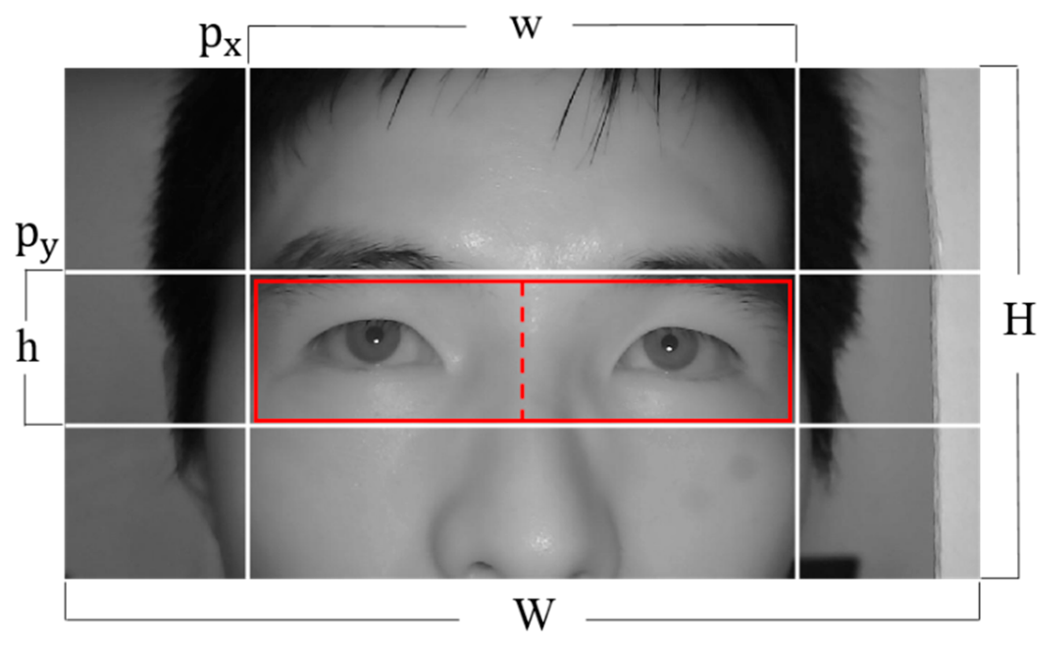
At this stage, a fixed sub-image containing the eye regions, while excluding regions of no interest (like nose and hair), is extracted to reduce the search space for the subsequent steps. In our system, the positions of the subject and the camera remain the same so that the data captured by the system show a high degree of consistency, that is, half of the face from the tip of the nose to the hair occupies the middle area of the image. This information, known as a priori, together with the anthropometric relations, can be used to quickly identify the rough eye regions. The boundary of the eye regions can be defined as

$${\mathrm{p}}_{\mathrm{x}}=0.2\times \mathrm{W},{\mathrm{p}}_{\mathrm{y}}=0.4\times \mathrm{H},\mathrm{w}=0.6\times \mathrm{W},\mathrm{h}=0.3\times \mathrm{H},$$

(1)

where W and H are the width and height of the image, w and h are the width and height of the eye regions, and $\left({\mathrm{p}}_{\mathrm{x}},{\mathrm{p}}_{\mathrm{y}}\right)$ defines the top-left position of the eye regions, respectively, as shown in Figure 3.

Thus, the eye regions are extracted, and the right and left eye can be distinguished by dividing the area into two parts, of which the area with smaller x coordinate corresponds to the right eye and vice versa, by comparing the x coordinates of the left upper corner of both eye regions.

3.2. Iris Measure and Template Detection

During this stage, the measure and template of the iris are detected. To achieve this, it is necessary to locate the iris boundary, particularly, the boundary of iris and sclera. The flowchart of this stage is shown in Figure 4. (1) First, the eye image is converted from RGB to grayscale. (2) Then the Haar-like feature is applied to the grayscale image to detect the exact eye region with the objective of further narrowing the area of interest. This feature extraction depends on the local feature of the eye, that is, the eye socket appears much darker in grayscale than the area of skin below it. The width of the rectangle window is set to be approximately the horizontal length of the eye, while the height of the window is variable within a certain range. The maximum response of this step corresponds to the eye and the skin area below it. (3) The Gaussian filter is applied to the result of (2), with the goal of smoothing and reducing noise. (4) Then, the canny method is applied as an edge-highlighting technique. (5) The circular Hough transform is employed to locate the iris boundary, due to its circular character. In performing this step, only the vertical gradients (4) are taken for locating the iris boundary [32]. This is based on the consideration that the eyelid edge map will corrupt the circular iris boundary edge map, because the upper and lower iris regions are usually occluded by the eyelids and the eyelashes. The eyelids are usually horizontally aligned. Therefore, the technique of excluding the horizontal edge map reduces the influence of the eyelids and makes the circle localization more accurate and efficient. (6) Subsequently, we segment a region with dimensions of 1.2× radius, horizontally, and 1.5× radius, vertically, on both sides from the iris center in the original gray image. The radius and iris center used in this step are the radius and center coordinates of the iris region detected in the last step. These values were chosen so that a complete iris region could be segmented without any damage. This region will be used as a template for the next stage.

The above operations are applied on the right and left eye regions, respectively, in a ten-frame interval, and ten pairs of iris radius values are extracted. The interval should be chosen to meet two conditions. First, the radius should be accurately determined in the interval. Second, the interval should not influence the next stage because the segmented region will be used for template matching. By the end of the interval, the iris radius value with the largest frequency is determined as the final iris radius. Thus, we have the right iris and left iris, with the radius of ${\mathrm{R}}_{\mathrm{r}}$ and ${\mathrm{R}}_{\mathrm{l}}$, respectively.

3.3. Key Frame Detection

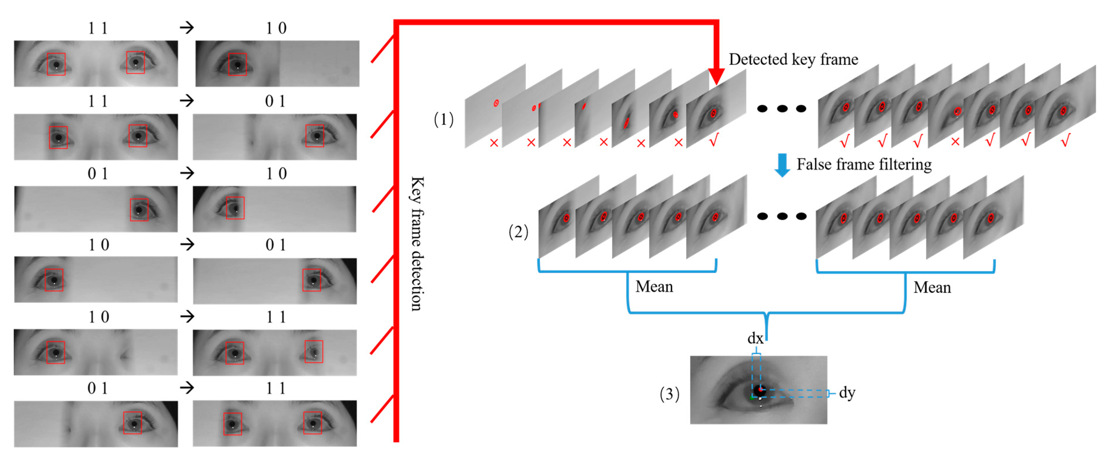
At this stage, the key frame detection is performed with the template matching technique on the eye region. The cover test is essentially a stimulus-response test. What we are interested in is whether the eye movements occur when a stimulus occurs. In the system, an entire process of tests is recorded in the video, which contains nearly 3000 frames at a length of about 50 s. We examined all frames between two stimuli. The stimuli we focused on are the unilateral cover test for the left and right eye, the alternating cover test for left and right eye, and the cover-uncover test for the left and right eye. In total, 18 stimuli are obtained with 6 types of stimuli for 3 rounds. The useful information accounts for about two-fifth of the video. Therefore, it is more efficient for the algorithm to discard these redundant information. The key frame detection is for the purpose of finding the frame where the stimulus occurs.

The right iris region segmented in Section 3.2 is used as a template, and the template matching is applied to the eye regions. The thresholds ${\mathrm{TH}}_1$, ${\mathrm{TH}}_2$ are set for the right eye region and the left region, respectively, and ${\mathrm{TH}}_2$ is smaller than ${\mathrm{TH}}_1,$as the right iris region is used as a template. The iris region is detected if the matching result is bigger than the threshold. In the nearby region of the iris, there may be many matching points which present the same iris. The repeated point can be removed by using the distance constraint. Therefore, the number of the matching template is consistent with the actual number of irises. The frame number, the number of iris detected in the right eye region, the number of the iris detected in the left region are saved in memory. Then we search the memory to find the position of the stimulus. Taking the unilateral cover test for the left eye as an example, the number of iris detected is [1 1], separately, before the left eye is covered and then [1 0], after covering the left eye. Therefore, we can use the state change from [1 1] to [1 0] to determine the corresponding frame of the stimuli. The correspondence between state changes and stimulus is shown in

Table 1. State changes and stimulus.

State Change	Stimuli
[1 1] → [1 0]	Covering the left eye in unilateral cover test
[1 1] → [0 1]	Covering the right eye in unilateral cover test
[0 1] → [1 0]	Uncovering the right eye in alternate cover test
[1 0] → [0 1]	Uncovering the left eye in alternate cover test
[1 0] → [1 1]	Uncovering the left eye in cover-uncover test
[0 1] → [1 1]	Uncovering the right eye in cover-uncover test

. Thus, the frame number of the eighteen stimulus can be obtained.

3.4. Pupil Localization

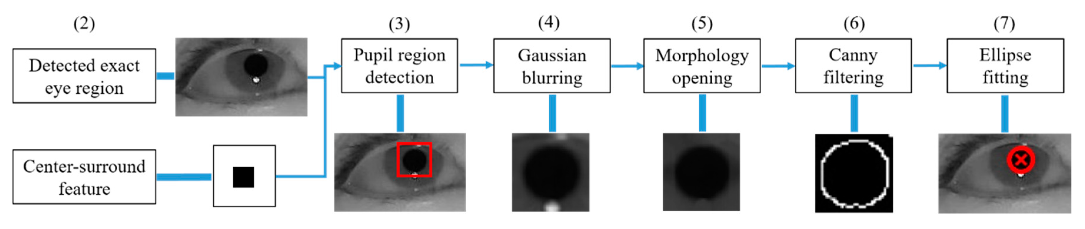
The pupil localization process is used to locate the pupil, which is the dark region of the eye controlling the light entrance. The flowchart of this stage is shown in Figure 5. (1) First, the eye image is converted into grayscale. (2) The Haar-like rectangle feature, same as that in Section 3.2, is applied to narrow the eye region. (3) Then another Haar-like feature, the center-surround feature with the variable inner radius of r and outer radius of 3r, is applied to the detected exact eye region of step 2. This feature makes use of the pupil being darker than the surrounding area. Therefore, the region corresponding to the maximum response of the Haar feature is a superior estimate of the iris region. The center coordinates and radius of the Haar feature is obtained and a region can be segmented with a dimension of 1.2× radius, horizontally and vertically, on both sides from the center of the detected region, to make sure the whole pupil is in the segment. Then we perform the following techniques. (4) Gaussian filtering is used to reduce noise and smooth the image while preserving the edges. (5) The morphology opening operation is applied to eliminate small objects, separate small objects at slender locations, and restore others. (6) The edges are detected through the Canny filter, and the contour point is obtained.

Given a set of candidate contour points of the pupil, the next step of the algorithm is to find the best fitting ellipse. (7) We applied the Random Sample Consensus (RANSAC) paradigm for ellipse fitting [33]. RANSAC is an effective technique for model fitting in the presence of a large but unknown percentage of outliers, in a measurement sample. In our application, inliers are all of those contour points that correspond to the pupil contour and outliers are contour points that correspond to other contours, like the upper and the lower eyelid. After the necessary number of iterations, an ellipse is fit to the largest consensus set, and its center is considered to be the center of the pupil. The frame number and pupil center coordinates are stored in memory.

3.5. Deviation Calculation

In order to analyze the eye movement, the deviation of the eyes during the stimulus process needs to be calculated. During a stimulus process, the position of the eye remains motionless before the stimulus occurs; after stimuli, the eye responds. The response can be divided into two scenarios. For the simpler case, the eyeball remains still. For the more complex case, the eyeball starts to move after a short while and then stops moving and keeps still until the next stimuli. Based on the statistics in the database, the eyes complete the movement within 17 frames and the duration of the movement is about 3 frames.

The schematic of deviation calculation is shown in Figure 6. The pupil position data within the region from the 6 frames before the detected key frame, to 60 frames after the key frames, are selected as a data matrix. Each row of the matrix corresponds to the frame number, the x, y coordinate of the pupil center. Next, an iterative process is applied to filter out the singular values of pupil detection. The current line of the matrix is subtracted from the previous line of the matrix, and the frame number of the previous line, the difference between the frame numbers Δf, and the difference between the coordinates Δx, Δy are retained. If $\Delta \mathrm{x}>\Delta \mathrm{f}.\mathrm{v}$, where v is the statistical maximum of the offset of pupil position of two adjacent frames, then this frame is considered to be wrong and the corresponding row in the original matrix is deleted. This process iterates until no rows are deleted or the number of loops exceeds 10. Finally, we use the average of the coordinates of the first five rows of the reserved matrix as the starting position and the average of the last five rows as the ending position, thus, obtaining the deviation of each stimulus, as expressed by the equations:

$$\begin{gathered} {\mathrm{Dev}}_{\mathrm{p}}^{\left(\mathrm{x}\right)}=|{\mathrm{x}}_{\mathrm{e} }-{\mathrm{x}}_{\mathrm{s}}|; \\ {\mathrm{Dev}}_{\mathrm{p}}^{\left(\mathrm{y}\right)}=\left|{\mathrm{y}}_{\mathrm{e}}- {\mathrm{y}}_{\mathrm{s}}\right|, \end{gathered}$$

(2)

where ${\mathrm{x}}_{\mathrm{e}}$and ${\mathrm{y}}_{\mathrm{e}}$ are the ending positions of the eye in a stimulus, the ${\mathrm{x}}_{\mathrm{s}}$ and ${\mathrm{y}}_{\mathrm{s}}$ are the starting positions of the eye, and ${\mathrm{Dev}}_{\mathrm{p}}^{\left(\mathrm{x}\right)}$,${\mathrm{Dev}}_{\mathrm{p}}^{\left(\mathrm{y}\right)}$ are the horizontal and vertical deviations in pixels, respectively.

3.6. Strabismus Detection

Obtained deviation of each stimulus, the deviation value in pixel ${\mathrm{Dev}}_{\mathrm{p}}$ can be converted into prism diopters ${\mathrm{Dev}}_{\Delta }$, which is calculated out using the equation:

$${\mathrm{Dev}}_{\Delta }=\left(\frac{{\mathrm{DE}}_{\mathrm{m}\mathrm{m}}}{{\mathrm{DE}}_{\mathrm{p}}}\right)·\mathrm{dpMM}·{\mathrm{Dev}}_{\mathrm{p}},$$

(3)

where ${\mathrm{DE}}_{\mathrm{mm}}$ is the value of the mean diameter of iris boundary of adult patients and ${\mathrm{DE}}_{\mathrm{mm}}=11\mathrm{mm}$ [34], ${\mathrm{DE}}_{\mathrm{p}}$ is the diameter value of the iris boundary detected in pixels, dpMM is a constant in millimeter conversion for prismatic diopters ($\Delta /\mathrm{mm}$) and $\mathrm{dpMM}=15\Delta$ [35]. Finally, we have the deviation ${\mathrm{Dev}}_{\Delta }$ expressed in diopter.

The subject’s deviation values are calculated separately for different cover tests. The subject’s deviation value for each test is the average of the deviations calculated for both eyes. These values are used to detect the presence or absence of strabismus.

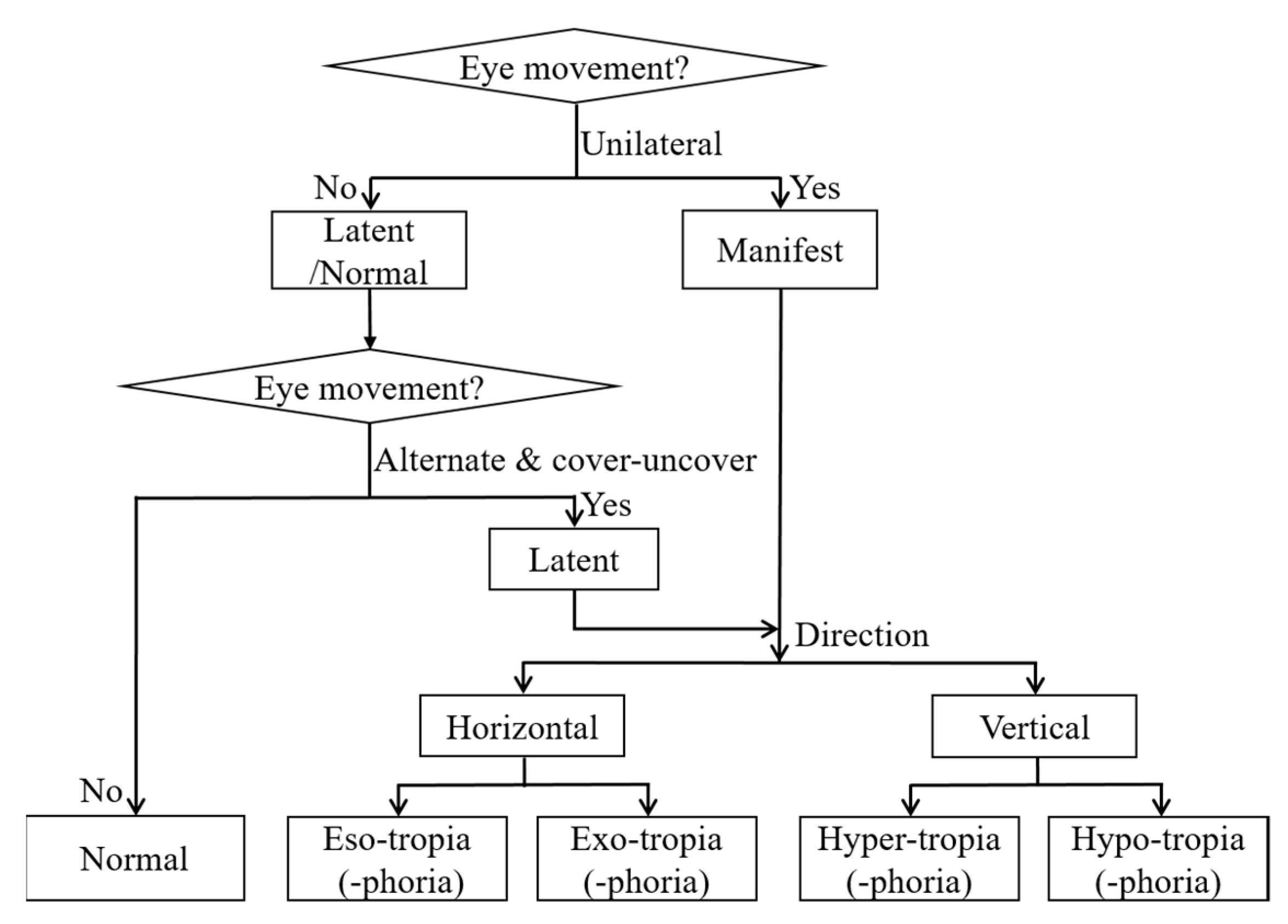
The types of the strabismus can first be classified as manifest strabismus or latent strabismus. According to the direction of deviation, it can be further divided into—horizontal eso-tropia (phoria), exo-tropia (phoria), vertical hyper-tropia (phoria), or hypo-tropia (phoria). The flowchart of the judgment of strabismus type is shown in Figure 7. If the eyes move in the unilateral cover test, the subject will be considered to have manifest strabismus and the corresponding type can be determined too, so it is unnecessary to consider the alternate cover test and the cover-uncover test and assessment ends. Nevertheless, if the eye movement does not occur in the unilateral test stage, there is still the possibility of latent strabismus, in spite of the exclusion of the manifest squint. We proceed to explore the eye movement in the alternating cover test and cover-uncover test. If the eye movement is observed, the subject is determined with heterophoria and then the specific type of strabismus is given on the basis of the direction of eye movement. If not, the subject is diagnosed as normal.

4. Experimental Results

In this section, the validation results of the intelligent strabismus evaluation method are presented, including the results of iris measure, key frame detection, pupil localization, and the measurement of the deviation of strabismus. In order to verify the effectiveness of the proposed automated methods, the ground truths of deviations in prism diopters were provided by manually observing and calculating the deviations of eyes for all samples. The measures of the automated methods have been compared with the ground truths.

4.1. Results of Iris Measure

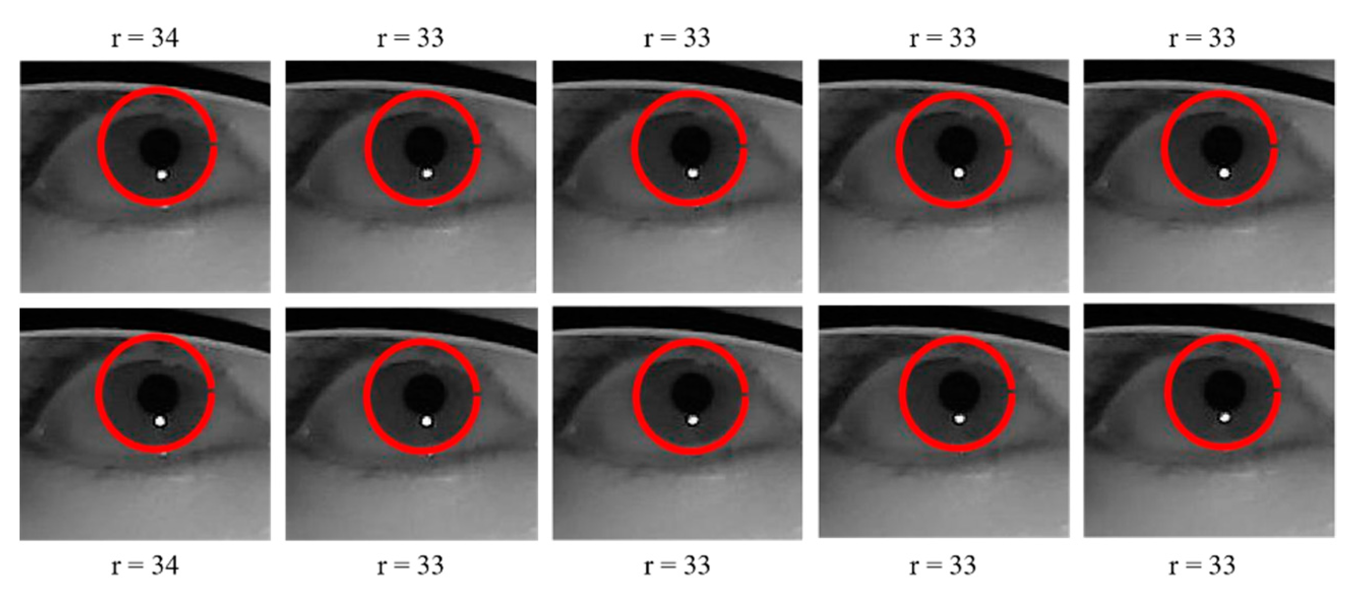
With the eye regions extracted, an accuracy of 100% was achieved in detecting the iris measure. The range of values that defines the minimum and maximum radius size for Hough transform was empirically identified to be between 28 and 45 pixels, for our database. Due to our strategy for choosing the radius with the largest frequency in the interval, the radius of the iris could be accurately obtained even if there were individual differences or errors. An example of the iris measure in 10 consecutive frames is shown in Figure 8. As can be seen from the figure, in an interval of 10 frames, there were 8 frames detected with a radius of “33” and 2 frames detected with a radius of “34”, so the radius of the iris was determined to be 33.

4.2. Results of Key Frame Detection

In order to measure the accuracy of the key frame detection, the key frames of all samples observed and labeled, manually, were regarded as the ground truths. The distance ${\mathrm{D}}^{\left(\mathrm{f}\right)}$ of the key detected frame ${\mathrm{f}}_{\mathrm{p}}$ and the manual ground truths ${\mathrm{f}}_{\mathrm{g}}$, was calculated using the equation:

$${\mathrm{D}}^{\left(\mathrm{f}\right)}=\left|{\mathrm{f}}_{\mathrm{p}}-{\mathrm{f}}_{\mathrm{g}}\right|$$

(4)

The accuracy of the key frame detection could be measured by calculating the percentage of the key frames for which the distance ${\mathrm{D}}^{\left(\mathrm{f}\right)}$ was within a threshold in the frames. The accuracy of the key frame detection for each cover test was given, as shown in

Table 2. The accuracy of the key frame detection for cover tests.

	Unilateral Cover Test	Alternating Cover Test	Cover-Uncover Test
${\mathbf{D}}^{\left(\mathbf{f}\right)}\le \mathbf{2}$	93.1%	62.5%	85.4%
${\mathbf{D}}^{\left(\mathbf{f}\right)}\le \mathbf{4}$	97.9%	88.2%	89.6%
${\mathbf{D}}^{\left(\mathbf{f}\right)}\le \mathbf{6}$	97.9%	97.2%	91.0%

.

Taking the unilateral cover test as an example, the detection accuracy was 93.1%, 97.9%, and 97.9%, at a distance of within 2, 4, and 6 frames, separately. As we can see, the detection rate in the alternating cover test was lower than that in others within the 2 and 4 frames intervals. This could be attributed to the phantom effects which might occur with the rapid motion of the occluder. It might interfere with the detection in the related frames, as the residual color of the trace left by the occluder merges with the color of the eyes. The movement of the occluder between two eyes brings more perturbation than that on one side. The detection rate appears good results for each cover test when the interval is set within 6 frames. As the deviation calculation method (Section 3.5) relaxes the reliance on key frame detection, our method could get a promising result.

4.3. Results of Pupil Localization

The accuracy of the proposed pupil detection algorithm was tested on static eye images on the dataset we built. The dataset consists of 5795 eye images with a resolution of 300$\times$150 pixels for samples without wearing corrective lenses and 400$\times$200 pixels for samples wearing lenses. All images were from our video database. The pupil location was manually labeled as the ground truth data for analysis.

In order to appreciate the accuracy of the pupil detection algorithm, the Euclidean distance ${\mathrm{D}}_{\mathrm{p}}^{\left(\mathrm{E}\right)}$ between the detected and the manually labeled pupil coordinates, as well as the distance ${\mathrm{D}}_{\mathrm{p}}^{\left(\mathrm{x}\right)}$ and ${\mathrm{D}}_{\mathrm{p}}^{\left(\mathrm{y}\right)}$on both axes of the coordinate system was calculated for the entire dataset. The detection rate measured in individual directions had a certain reference value, as the mobility of eyes has two degrees of freedom. The accuracy of the pupil localization could be measured by calculating the percentage of the eye pupil images for which the pixel error was lower than a threshold in pixels. We compared our pupil detection method with the classical Starburst [33] algorithm and circular Hough transform (CHT) [36]. The performance of pupil localization with different algorithms is illustrated in

Table 3. Performance of pupil localization with different algorithms on our dataset.

Method	${\mathbf{D}}_{\mathbf{p}}^{\left(\mathbf{E}\right)}<5$	${\mathbf{D}}_{\mathbf{p}}^{\left(\mathbf{E}\right)}<10$	${\mathbf{D}}_{\mathbf{p}}^{\left(\mathbf{x}\right)}<4$	${\mathbf{D}}_{\mathbf{p}}^{\left(\mathbf{y}\right)}<2$
Starburst [33]	27.0%	44.2%	39.9%	27.8%
CHT [36]	84.6%	85.0%	84.6%	83.4%
Ours	86.6%	94.3%	90.6%	80.7%

. The accuracy rates of the following statistical indicators were used: $“{\mathrm{D}}_{\mathrm{p}}^{\left(\mathrm{E}\right)}<5”$ and $“{\mathrm{D}}_{\mathrm{p}}^{\left(\mathrm{E}\right)}<10”$ corresponded to the detection rate, at 5 and 10 pixels, in Euclidean distance; “${\mathrm{D}}_{\mathrm{p}}^{\left(\mathrm{x}\right)}<4”$ or $“{\mathrm{D}}_{\mathrm{p}}^{\left(\mathrm{y}\right)}<2”$ represented the percentage of the eye pupil images for which the pixel error was lower than 4 pixels in horizontal direction or 2 pixels in vertical direction.

As we can see, the performance of the Starburst algorithm was much poorer, which was due to the detection of the pupil contour points, using the iterative feature-based technique. In this step, the candidate feature points that belonged to the contour points were determined along the rays that extended radially away from the starting point, until a threshold $\varnothing =20$was exceeded. For our database, there were many disturbing contour points detected, especially the limbus. This could cause the final stage to find the best-fitting ellipse for a subset of candidate feature points by using the RANSAC method to misfit the limbus. The performance of the CHT was acceptable, but it was highly dependent on the estimate of the range of the radius of the pupil. There might have been overlaps between the radius of the pupil and the limbus for different samples, which made the algorithm invalid for some samples. While our method shows a good detection result overall.

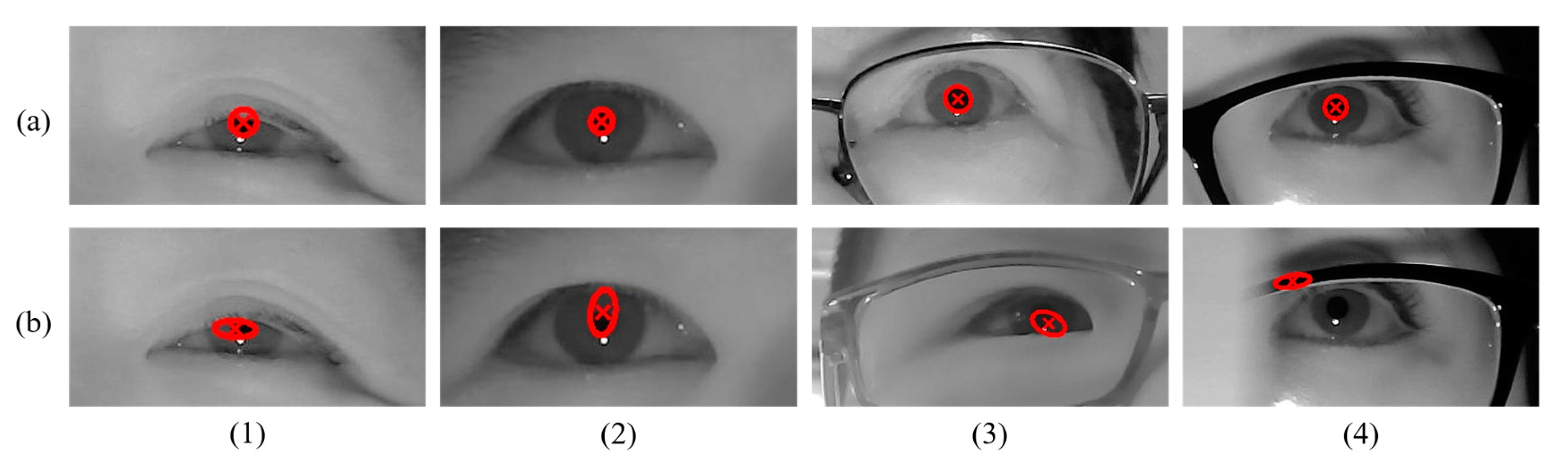
Actually, the overall detection rate was an average result. Poor detection in some samples had lowered the overall performance. Listed below, are some cases in locating the pupil, as shown in Figure 9. Some correct detection results are shown in Figure 9a, which shows that our algorithm could get a good detect effect in most cases, even if there was interference from glasses. Some typical examples of errors are described in Figure 9b. The errors could be attributed to the following factors—(1) a large part of the pupil was covered by the eyelids so that the exposed pupil contour, together with a part of eyelid contour, were fitted to an ellipse when the model was fitted, as shown in set 1 of Figure 9b; (2) the pupil was extremely small, so the model fitting was prone to be similar to the result discussed in factor 1, as shown in set 2 of Figure 9b; (3) the difference within the iris region was not so apparent that the canny filter could not get a good edge of the pupil, thus, leading to poor results, as shown in set 3 of Figure 9b; (4) the failure detection caused by the phantom effects when the fast-moving occluder was close to the eyeball, as shown in set 4 of Figure 9b.

4.4. Results of the Deviation Measurement

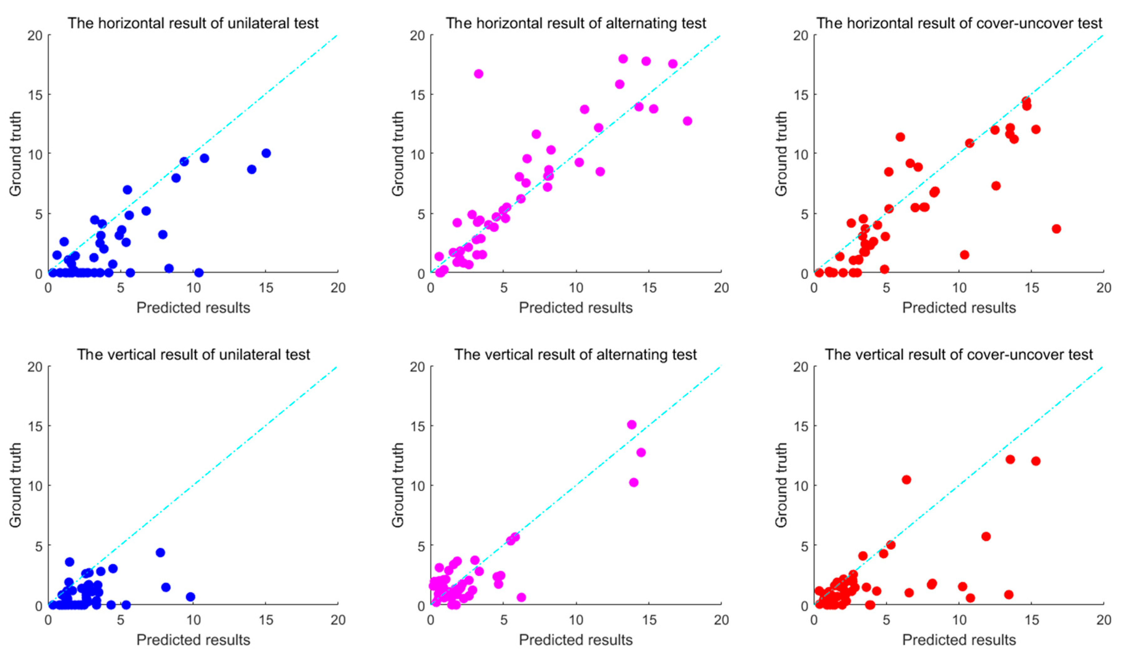
For analyzing the accuracy of the deviation calculated by the proposed method, the deviation of each stimulus was calculated as ground truth, by manually determining the starting position and ending position of each excitation for all samples, and labeling the pupil position of the corresponding frames, and then calculating the strabismus degrees in prism diopters. The deviations of the automated method were compared with the ground truths. The accuracy of the deviation measurement was measured by calculating the percentage of deviations for which the error of the deviation detected and manual ground truths was lower than a threshold.

The accuracy rate using different indicators are shown in

Table 4. The accuracy rate of deviation calculation in prism diopters (∆) for different cover test stages in the horizontal direction.

(∆)	$\mathit{E}\mathit{r}\mathit{r}\mathit{o}\mathit{r}<4$	$\mathit{E}\mathit{r}\mathit{r}\mathit{o}\mathit{r}<8$	$\mathit{E}\mathit{r}\mathit{r}\mathit{o}\mathit{r}<12$
Unilateral	81.3%	95.8%	97.2%
Alternate	85.4%	93.8%	97.9%
Uncover	74.3%	91.7%	96.5%

and

Table 5. The accuracy rate of deviation calculation in prism diopters (∆) for different cover test stages in the vertical direction.

(∆)	$\mathit{E}\mathit{r}\mathit{r}\mathit{o}\mathit{r}<2$	$\mathit{E}\mathit{r}\mathit{r}\mathit{o}\mathit{r}<4$	$\mathit{E}\mathit{r}\mathit{r}\mathit{o}\mathit{r}<6$
Unilateral	70.1%	88.2%	94.4%
Alternate	71.5%	93.8%	96.5%
Uncover	68.8%	86.1%	88.2%

. For example, “$error<2$” represents the percentage of the deviation calculation for which the error in prism diopters was lower than the threshold 2 in certain axes, and so on. The indicators for vertical direction was set to be more compact as the structure of the eye itself causes it to have a smaller range of motion in the vertical direction than that in the horizontal direction. The calculation accuracy was acceptable when the error was set to be 8$\Delta$ in the horizontal direction or 4$\Delta$ in the vertical direction. This conclusion could also be seen from Figure 10, which shows the correlation of deviation between the ground truth and the predicted results. Each point represents the average of three stimuli. It can be seen that most of the points were within the 8$\Delta$ or 4$\Delta$ error, and it could be considered an error as the points were outside the range. The results demonstrated a high consistency between the proposed method and the manual measurement of deviation, and that the proposed methods were effective for automated evaluations of strabismus.

5. Conclusions and Future Work

In this paper, we proposed and validated an intelligent measurement method for strabismus deviation in digital videos, based on the cover test. The algorithms were applied to video recordings by near-infrared cameras, while the subject performed the cover test for a diagnosis of strabismus. In particular, we focused on the automated algorithms for the identification of the extent to which the eyes involuntarily move when a stimulus occurs. We validated the proposed method using the manual ground truth of deviations in prism diopters, from our database. Experimental results suggest that our automated system can perform a high accuracy of evaluation of strabismus deviation.

Although the proposed intelligent evaluation system for strabismus could achieve a satisfying accuracy, there are still some aspects to be further improved in our future work. First, for the acquisition of data, there are obvious changes in the video brightness, due to the cover of the occluder. For example, almost half of the light was blocked when one eye was covered completely. This might bring a perturbation for the algorithm, especially for the pupil detection. Therefore, our system needed to be further upgraded to reduce this interference. Second, the subjects were required to remain motionless while the cover test is performed. In fact, a slight movement of the head that is not detectable to humans will cause a certain deviation in the detection of eye position, thus, reducing the accuracy of the final evaluation. To develop a fine eye localization, eliminating slight movements would improve the result. Additionally, our system can also be used for an automatic diagnosis of strabismus, in the future.