Abstract
Liquefaction is one of the most destructive phenomena caused by earthquakes, and it has been studied regarding the issues of risk assessment and hazard analysis. The strain energy approach is a common method to evaluate liquefaction triggering. In this study, the response surface method (RSM) is applied as a novel way to develop six new strain energy models in order to estimate the capacity energy required for triggering liquefaction (W), based on laboratory test results collected from the literature. Three well-known design of experiments (DOEs) are used to build these models and evaluate their influence on the developed equations. Furthermore, two groups of artificial neural network (ANN) and RSM models are derived to investigate the complicated influence of fine content (FC). The first group of models is based on a database without limitation on the range of input parameters, and the second group is based on a database with FC lower than the critical value of 28%. The capability and accuracy of the six presented models are compared with four existing models in the literature by using additional new laboratory test results (i.e., 20 samples). The results indicate the superior performance of the presented RSM models and particularly the second group of the models based on a limited value of FC.
1. Introduction
Liquefaction is one of the most destructive effects of earthquakes. This phenomenon, which has occurred several times during recent earthquakes, is caused by seismic shear waves that propagate upward to the surface layers, increasing pore water pressure in saturated, relatively loose or loose sandy deposits. Liquefaction occurs when rapid earthquake motion prevents drainage, thereby increasing excess pore water pressure to as much as initial overburden stress. Liquefaction causes severe property damage and fatalities. After liquefaction, the strength and stiffness of the liquefied soil are considerably decreased, often resulting in a range of structural failures. Evaluating the liquefaction potential guides the decision of which method is to be applied to prevent the disaster.
A number of approaches and models have been presented to assess the liquefaction potential of soils. Some of these approaches follow a stress-based procedure, on the basis of the equation presented by Seed and Idriss [1]. During this process, the shear stress induced by an earthquake is first determined according to the peak ground surface acceleration (amax). Then, the cyclic stress ratio (CSR) and the cyclic shear strength (CRR) are determined, and by comparing them the potential of liquefaction is analyzed [2,3,4,5,6,7,8,9,10,11]. Strain-based methods have also been conducted by supposing that pore water pressure grows by control of the cyclic shear strain during dynamic loads [12,13].
In contrast, other researchers have assessed the potential of liquefaction through an energy-based method, which considers the energy dissipated into the soil by earthquake motions. This method can be divided into three groups based on case histories during earthquakes that occurred in the past [14,15,16], the Arias intensity (Ih) [17,18], and laboratory test results [19,20]. Shafee et al. [21] performed some uniaxial shaking tests and demonstrated that the difference between strain energy generated in the soil caused by biaxial and uniaxial shaking tests is negligible. Zheghal et al. [22] studied the effect of non-proportionality and the phase angle of the induced shear stresses on rising pore water pressure. Moreover, researchers investigated the influence of five parameters, including the initial effective mean confining pressure (), initial relative density (Dr)%, fine content (FC)%, coefficient of uniformity (Cu), and mean grain size (D50), on the capacity energy of soils (W) [13,23,24,25,26,27,28,29,30,31] by considering laboratory test results. Baziar et al. [26] collected a large number of datasets with a wide range of test results, including six parameters, and they divided them randomly into a testing and training phase in order to present artificial neural networks (ANNs). Furthermore, they eliminated the coefficient of curvature (Cc) due to no increase in the model’s accuracy, and they presented new artificial neural network (ANN) and multi-linear regression (MLR) models, including five parameters containing , Dr%, FC%, Cu, and (D50) in mm. With the same dataset collected by Baziar et al. [26], Alavi et al. [28] developed three new models. By adding new data to the dataset of Baziar et al. [26] and applying a neuro-fuzzy interface system (ANFIS), Cabalar et al. [32] developed a model that included six parameters containing Cc and demonstrated its influence. However, data division was conducted randomly in all studies, without considering the statistical aspects of parameters. Furthermore, data was divided into two groups, testing and training, without performing a validating phase to prevent overtraining of the ANN model. A validating phase is applied to minimize overfitting of the trained model [33,34]. In addition, Tao [35] investigated the complicated influence of FC and illustrated that liquefaction resistance, in terms of the unit energy, starts to increase with an increase in FC above 28%. They also indicated that the liquefaction resistance becomes less dependent on relative density when FC is less than 28%. Maurer et al. [36] investigated 7000 dataset case histories from the 2010–2011 Canterbury Earthquakes and indicated that the evaluation of liquefaction is less accurate when soils have a high FC value. Although these studies have indicated an altered influence of a high FC value on liquefaction assessment, it has not yet been taken into account to propose a model.
In this study, a larger dataset is first collected. Then, to evaluate the influence of FC on W, two ANN models are constructed that include the following six input parameters: , Dr%, FC%, Cu, D50, and Cc. To analyze the complicated influence of FC, the first ANN model, without any constraints in the range of input parameters, is derived similarly to other studies that have been performed and explained herein, and the second ANN model is derived through a database with FC values less than 28%, as in Tao [35]. To increase the accuracy and capability of the ANN models, the dataset is divided into three groups by considering the statistical aspects of parameters with similar mean as well as mean coefficient of variation (COV) values, instead of random division. The first group is for the training phase, the second is for testing, and the third is for the validating phase, to prevent overtraining in the training phase. In the second step, six visualized equations are captured by using the response surface method (RSM), which was demonstrated to be a capable method for evaluating liquefaction in sandy soil by Pirhadi et al. [37]. To the best of our knowledge, no other studies have been conducted on liquefaction using RSM. In Section 5, the dataset and two derived ANN models and their characteristics are described. According to any ANN model, three different design of experiments (DOEs) are performed. Therefore, three equations are obtained to illustrate and calculate correlation between six defined parameters and W as a target. During this step, the meaningfulness of all terms of the equations are analyzed through hypothesis testing, and to obtain more capable and reliable equations, some equation terms that do not provide a meaningful correlation with the target are eliminated, instead of performing an overall elimination of parameters such as Cc. The final equations thus contain all six parameters and are presented in Section 6. Furthermore, by applying three different DOEs, their influence and capability are studied to determine the best DOE that can be applied for similar issues. Finally, to demonstrate the accuracy and capability of the presented equations, their predicted results are compared with four existing, well-known, and highly rated models that are currently used. Section 7 presents this comparison, using 20 samples from Dief [38] that are not included in the database to develop the ANN and RSM models for this study. Figure 1 illustrates the flowchart of the process applied in this study to develop the RSM equations.
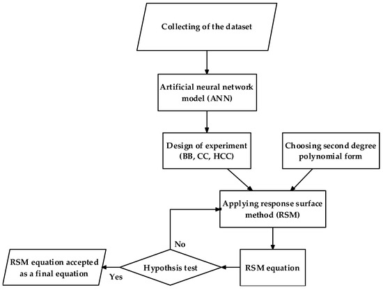
Figure 1.
Flowchart of the process to derive the response surface method (RSM) equations in this study; BB: Box-Behnken; CC: central composite; HCC: half central composite.
2. Approaches Based on Laboratory Test Results
By inspecting and monitoring the number of site responses to earthquakes’ time history accelerations in the West of the United States and by introducing normalized maximum energy, which is the area under the stress–strain of earthquake motion at depths, Alkahtib [39] derived a relationship between maximum energy, Dr, amax, and initial effective confining stress.
Additionally, Liang [13] derived the equations by performing 74 torsional shear tests on Reid Bedford sand, Lower San Fernando Dam (LSFD) silty sand, and Lapis Luster dried sand (LSI-30):
Reid Bedford:
Reid Bedford sand:
LSFD sand:
LSI-30 sand:
where δW is the cumulative unit energy (J/m3), Γ is the shear strain amplitude, and R2 is the coefficient of determination.
Furthermore, by conducting 27 strain-controlled torsional triaxial tests on Reid Bedford sand, Kusky [23] derived the following two regression equations:
where f is the cyclic rate (Hz).
For the first time, Figueroa et al. [24] and Rokoff [25] inspected the influence of particle size distribution on the potential of liquefaction according to the strain energy-based procedures. Rokoff performed some cyclic torsional shear tests on the sand samples from Nevada, incorporating the Cu and the Cc, and the author presented the equations expressed as:
where Di is the particle diameter, which is given by a grain-size distribution for a given percent finer, denoted by the subscript i.
Through a statistical method, using the test results data of Liang [40] and Rokoff [25], Wallin [41] presented mathematical equations for Reid Bedford sand, LSFD silty sand, and Nevada sand.
Baziar et al. [26] collected a large database containing 284 cyclic, triaxial, torsional shear, and simple shear test results, and they developed two ANN models. Thereafter, by comparing the ANN models’ results with data from 18 centrifuge tests, they evaluated their model. Their first model included six input parameters—, Dr%, FC%, Cu, D50 (in mm), and Cc—and the output (the target) was W (J/m3). In the second model, they eliminated Cc and developed the model with the five extra input parameters.
With the same database as Baziar et al. [26] and using genetic programming (GP), linear genetic programming (LGP), and multi-expression programming (MEP), Alavi et al. [28] developed three equations to evaluate W. Cabalar et al. [32] utilized an ANFIS on the same database as Baziar et al. [26] and illustrated the effect of input parameters by graphical representation. By adding some new datasets to those of Baziar et al. [26] and by applying GP, Baziar et al. [27] developed an equation to estimate the W with the same parameters as those of Baziar et al [26]. Zhang et al. [29] applied multivariate adaptive regression splines (MARS), which is a nonparametric regression procedure, and by using a similar database to that of Baziar al. [26], they developed a model to measure W based on five input parameters, which are similar to the previously mentioned studies [26,27,32]. It should be mentioned that all models and equations presented in the previously mentioned studies [26,27,28,29,32] estimated the capacity energy (W) in a logarithm term (log W).
3. Artificial Neural Network
Neural networks are defined similarly to biological (brain) network systems, and they include three interconnected stages: (1) input layer, (2) hidden layer(s), and (3) output layer. In the first stage, input data are entered into the network and in the second stage, they are weighted and connected with hidden units. Finally, in the third stage, the output is predicted according to weights between the output units and hidden units. One of the most important actions and advantages of an ANN is the discovery of nonlinear, statistical data, complex relationships between input and output parameters, and its use in a variety of science and engineering applications, particularly recently [31,42,43,44,45,46,47]. To achieve this goal, a sufficient number of dataset samples are required to train the ANN with a suitable algorithm.
In this study, the backpropagation network that is the most common among multilayer perceptrons (MLPs) is applied [48]. The model is constructed with three layers: the input, hidden, and output (target) layer. Thus, a single hidden layer, which theoretical studies have demonstrated is sufficient to predicate all complex nonlinear functions [49], is used to develop the ANN models.
4. Response Surface Method
The RSM consists of mathematical and statistical techniques that originated from a graphical perspective that Box et al. [50] generated in the early 1950s. Researchers in a wide variety of science and industry fields have utilized it [51,52,53]. In this method, the volume of input parameters is fitted by experimental data, called DOE. Then, an empirical model is developed to define a relationship between the explanatory variables or input parameters and the output parameter(s) or target. To achieve this goal, some steps must be considered. They are briefly described next.
4.1. Selection of Regression Model Function
The mathematical framework function between the input variables and the target is called a regression model, and in cases with more than two variables, it is called a multiple regression model. In the first step, the mathematical regression framework with the best fit is selected. The most common models are as follows:
4.2. Design of Experiment
The DOE is applied to fit the model to all physical experiments. During this process, the points that must be entered into the RSM are defined [54]; in other words, both a series of samples containing all inputs and the targets calculated at special points must be prepared (response surface design). There are several types of DOEs, such as full factorial design, central composite (CC) design, D-optimal designs, Taguchi’s contribution to experimental design, and the Latin hypercube design. The type of DOE selected can affect the prediction result of the RSM, and it depends on the properties of the values and parameters. Furthermore, the Box-Behnken (BB) design [55] is an economical design that is common in industry. It only requires three levels for every parameter: −1, 0, and 1 correspond to each variable’s minimum, mean, and maximum values, respectively. The CC is the most commonly used design, and it contains the three levels of the BB design, with extra points for the distance of α from the center design. The half central composite (HCC) design is similar to the CC design; however, there is a difference in the center points and value of α. The HCC design also has similar properties to the CC design, with a different value for α.
4.3. Coding of the Input Variables
Each real value is transferred to the coordinates inside a scale with dimensionless values, called coding values, by the function described below:
where Yi is the coded value, Xi is the real value, Zi is the middle of the real value range, and L is the major coded limit value in the matrix for each variable.
4.4. Hypothesis Test
A formal process, called a hypothesis test, is employed to determine the appropriateness of rejecting the null hypothesis due to samples. In other words, there is an assumption, which could be true or false, and the procedure to accept or reject this assumption is the hypothesis test. The P-value is one of the most common ways of deciding. P-values are used in many areas of statistics, including basic statistics, linear and nonlinear models, reliability analyses, and multivariate analyses. In this study, the commonly used alpha value of 0.05 is considered. If the P-value of a test statistic is larger than the alpha, then the null hypothesis is accepted, and if it is less than the alpha, then the null hypothesis is rejected.
5. Databases and Artificial Neural Network Models
As previously mentioned, two databases were arranged for two groups of derived equations—both consisted of six parameters, namely , Dr%, FC%, Cu, D50 (in mm), and Cc—and the target was log W. Also, the criterion for the triggering of liquefaction is ru = 1 for the initiate of liquefaction or strain equal to 5% (εDA = 5%). The database that was used to develop the first group of equations includes 217 cyclic, triaxial laboratory test results [56]; 61 cyclic, torsional laboratory test results [22,57]; six cyclic simple tests [58], and 22 centrifuge test results [36]. In addition, new data were added from 22 samples from the VErification of Liquefaction Analysis by Centrifuge Studies (VELACS) program [25,35,58], along with 48 cyclic, triaxial laboratory test results [59], and 27 cyclic, torsional laboratory test results [35]. In total, the database was composed of 403 samples.
5.1. First Artificial Neural Network Model
To achieve a more accurate and capable model, the database was divided into three groups according to statistical characteristics, with similar mean and COV values. A backpropagation neural network algorithm with one hidden layer, which is the most common algorithm, was built to develop an ANN model for predicting the capacity energy (W) of soil liquefaction in the coded value of DOE to ultimately establish RSM equations. Approximately 14% of the database (60 samples) was selected for the testing stage; the same number was chosen for the validating stage, and an extra 287 samples were selected for training. The certificates and characteristics of the first database and the ANN model are listed in Table 1 and Table 2. It can be seen that FC ranges from zero to 100% in the first database. The R values for all three subsets are more than 90%, illustrating the strong performance of the model.

Table 1.
Characteristics of complete input parameters used for the first ANN model and RSM equation.
Table 2.
Characteristics of the ANN model for the first dataset.
5.2. Second Artificial Neural Network Model
In the second database, with similar parameters and as per Tao [35], the samples with an FC less than 28% were selected from the first database. Overall, the characteristics and certificates of the second database contain 309 samples, and the ANN model belongs to it, as illustrated in Table 3 and Table 4. As previously mentioned, the second dataset is created by eliminating all samples with an FC larger than 28% from the first dataset. The database was again divided into three groups for testing, validating, and training the ANN, with sample numbers of 44, 44, and 221, respectively. It should be noted that for all three groups of samples, sample division was performed with the same statistical factors, such as mean values and mean COV values, rather than randomly, to increase the accuracy of the ANN-trained model. Table 4 shows that the R values for the three subsets are larger than 90%, indicating the reasonable accuracy of the model to estimate W. The FC values in the second database, as shown in Table 3, range from zero to 26%. It should be noted that the second database is composed of 309 samples, whereas the first database has 403 samples. Therefore, the first ANN model was developed on the basis of a larger database.
Table 3.
Characteristics of the complete input parameters used for the second ANN model and RSM equation.
Table 4.
Characteristics of the ANN model for the second dataset.
6. The RSM Equations
The second-degree polynomial with cross-terms Equation (14) is selected to establish the RSM equations, due to it being the most capable and precise model. Based on the ANN models which are developed in this study and considering three DOEs, a total of 6 equations are derived. For the BB, CC, and HCC, 54, 90, and 53 coded samples, respectively, were constructed according to six input parameters in this study. Due to the lack of values of W in coded points, the ANN models were used to predict the targets of coded samples. Thereafter, three DOEs were performed to develop three equations to predict the (W) for any dataset. Then, by performing a hypothesis test through P-values, some terms of the original second-degree polynomial with cross-terms were eliminated. In this study, the common alpha value of 0.05, which many researchers have used, is considered. If the P-value of a test statistic is larger than the alpha, then the null hypothesis is accepted, whereas if it is less than the alpha, then the hypothesis is rejected. The RSM was then run repeatedly to establish the final equations, as presented in Table 5, Table 6, Table 7, Table 8, Table 9 and Table 10. Finally, their results were compared to other well-known models to demonstrate the accuracy and capability of the six presented equations herein.
Table 5.
RSM equation with the DOE of the BB design, based on the first ANN model (R2 = 79.83%, R2 [adjust] = 69.46%).
Table 6.
RSM equation with the DOE of the CC design, based on the first ANN model (R2 = 73.89%, R2 [adjust] = 66.81%).
Table 7.
RSM equation with the DOE of the HCC design, based on the first ANN model (R2 = 72.74%, R2 [adjust] = 60.62%).
Table 8.
RSM equation with the DOE of the BB design, based on the second ANN model (R2 = 96.49%, R2 [adjust] = 94.52%).
Table 9.
RSM equation with the DOE of the CC design, based on the second ANN model (R2 = 93.37%, R2 [adjust] = 91.80%).
Table 10.
RSM equation with the DOE of the HCC based on the second ANN model (R2 = 94.63%, R2 [adjust] = 92.02%).
The adjusted R2 demonstrates the power of the regression, taking into account the number of predictors. In other words, it is a modified version of the R2, and it is always lower than the R2; however, when it is closer to the R2, this demonstrates a greater accuracy and ability to predict. It must be considered that to use these equations to predict W, the real values of six input parameters must first be transferred to the coded value in Equation (16) below; then, the value of W can be estimated by substituting the coded value in the RSM equations presented in Table 5, Table 6, Table 7, Table 8, Table 9 and Table 10.
Both RSM equations presented in this study must be applied with caution:
- (1)
- Both RSM equations require soil properties and laboratory test results to estimate Dr%, FC%, Cu, D50 (in mm), and Cc.
- (2)
- (3)
- The second RSM equation is only applicable for samples with an FC value of less than 28%.
- (4)
- It is necessary to transfer the real value of the parameters to the coded value as in Equation (16), then input this into the equations to estimate the results.
7. Comparison of the Predicted Capacity Energy of Liquefaction between the RSM Equations and Existing Models
To demonstrate the capability and accuracy of the RSM equations presented in this study, their prediction values are compared with the GP, LGP, MEP [28], and MARS [29] models, which are presented in the Appendix A. This is undertaken using 20 samples from Dief [38], from Nevada sand and Reid Bedford sand, which were not included in the database used to develop the ANN and RSM models for this study. The 20 samples’ parameter values are listed in Table 11, and the predicted values are compared in Table 12.
Table 11.
The 20 samples from Dief [38] that were used for a comparison of models’ performance.
Table 12.
Predicted results of the six RSM equations and measured results of 20 samples.
To illustrate the capability and accuracy of different equations, the results are summarized in Table 13 according to root mean square error (RMSE), mean absolute error (MAE), and coefficient of correlation (R). Lower RMSE and MAE values testify to more accuracy, whereas a higher R indicates a higher accuracy. Extra models are considered herein including genetic programming (GP), linear genetic programming (LGP), and multi expression programming (MEP) all developed by Alavi et al. [27] and multivariate adaptive regression splines (MARS) which is presented by Zhang et al. [28].
Table 13.
Predicted results of four available models and measured results of 20 samples.
A comparison was conducted regarding the capability and accuracy of the predicted values for the capacity energy liquefaction of soil W between six new equations and other models. All results are summarized in Table 14.
Table 14.
Summary of comparison between six new RSM equations and four available models.
Figure 2, Figure 3, Figure 4, Figure 5, Figure 6, Figure 7, Figure 8, Figure 9, Figure 10 and Figure 11 provide a visual comparison of the results. The second group of equations, with a database limited to FC values of less than 28%, illustrated more accuracy than all DOEs conducted in this study, as can be seen in Figure 5, Figure 6 and Figure 7. The CC and BB designs also indicated higher accuracy in comparison with the HCC design, as shown in Figure 2, Figure 3, Figure 4, Figure 5, Figure 6 and Figure 7. Furthermore, the R value of 0.911 for the BB28 equation and the CC with 0.830, closely followed by the HCC and CC28 equations, with 0.792 and 0.722, respectively, demonstrated the highest precision.
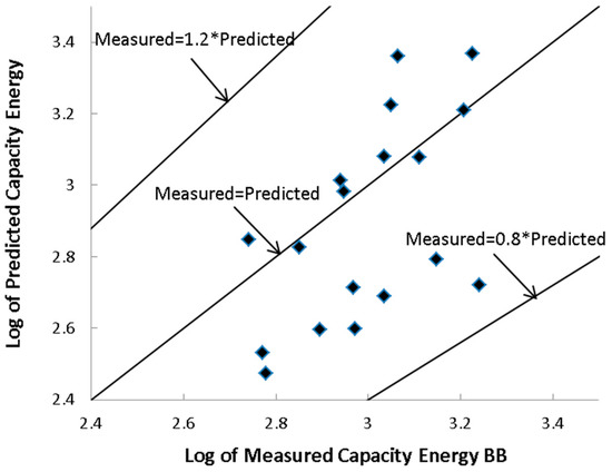
Figure 2.
Capacity energy predicted by RSM equation on the basis of the Box-Behnken DOE and the first ANN model versus the measured values of laboratory tests.
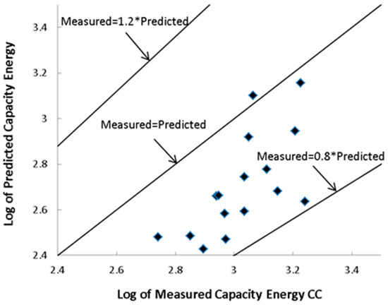
Figure 3.
Capacity energy predicted by RSM equation on the basis of the central composite (CC) design of experiment (DOE) and the first ANN model versus the measured values of laboratory tests.
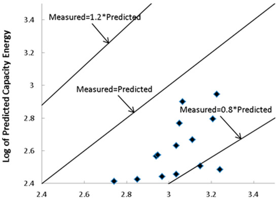
Figure 4.
Capacity energy predicted by RSM equation on the basis of the half central composite (HCC) design of experiment (DOE) and the first ANN model versus the measured values of laboratory tests.
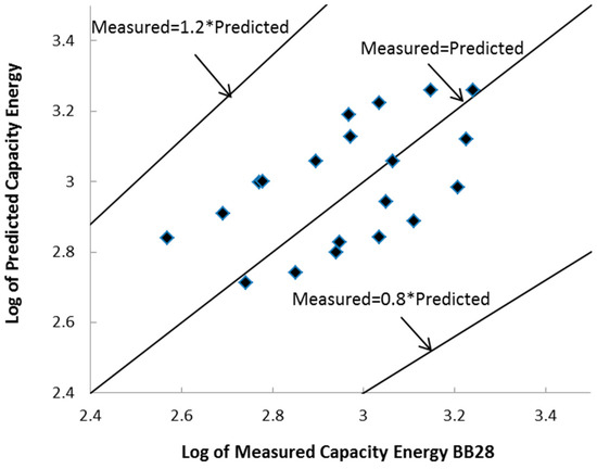
Figure 5.
Capacity energy predicted by RSM equation on the basis of the Box-Behnken (BB) design of experiment (DOE) and the second ANN model versus the measured values of laboratory tests.
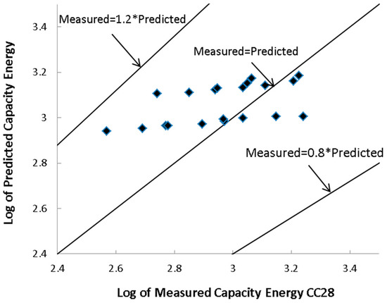
Figure 6.
Capacity energy predicted by RSM equation on the basis of the central composite (CC) and design of experiment (DOE) and the second ANN model versus the measured values of laboratory tests.
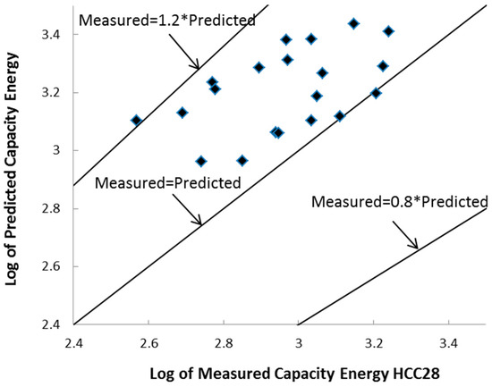
Figure 7.
Capacity energy predicted by RSM equation on the basis of half central composite (HCC) and design of experiment (DOE) and the second ANN model versus the measured values of laboratory tests.
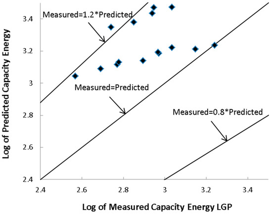
Figure 8.
Capacity energy predicted by genetic programming (LGP) versus the measured values of laboratory tests.
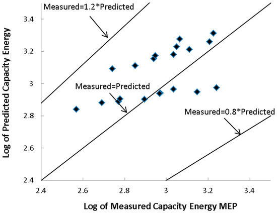
Figure 9.
Capacity energy predicted by multi expression programming (MEP) versus the measured values of laboratory tests.
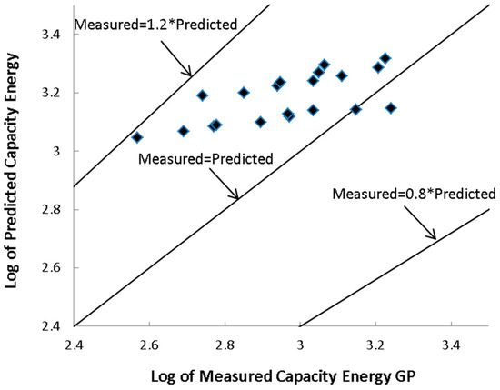
Figure 10.
Capacity energy predicted by genetic programming (GP) versus the measured values of laboratory tests.
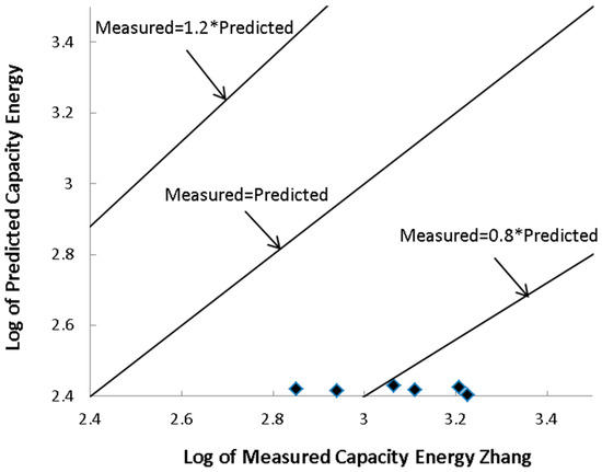
Figure 11.
Capacity energy predicted by Zhang’s equation versus the measured values of laboratory tests.
On the other hand, with RSME and MAE values of 0.173 and 0.139, respectively, CC28 demonstrated less inaccuracy. Considering the graphs, BB28 and CC28 were the most capable and accurate models among all six equations presented in this study as well as the four extra inspected models, as shown in Figure 2, Figure 3, Figure 4, Figure 5, Figure 6 and Figure 7. Moreover, five of the six RSM models demonstrated a higher R than the extra four models. The RMSEs of CC28, MEP, and BB28 were 0.173, 0.182, and 0.218, respectively, displaying the highest accuracy to predict W, as demonstrated in Table 14. In addition, the MAEs of CC28, MEP, and BB28—0.139, 0.157, and 0.203, respectively—revealed the most accuracy.
As can be seen from Figure 2, Figure 3, Figure 4, Figure 5, Figure 6, Figure 7, Figure 8, Figure 9, Figure 10 and Figure 11, among all models evaluated in this study, CC and HCC present underpredicted values for W. In contrast, HCC28 and LGP overstimated W in their predictions. Furthermore, BB28 shows the highest accuracy in predicting W.
8. Summary and Conclusions
In this study, a new tool, the response surface method (RSM), was used to develop six new equations to estimate the capacity energy of soil liquefaction (W). While the RSM has been used in industry, medicine, and science, according to the literature review, it has not been used to investigate soil liquefaction by other researchers. To examine the complicated influence of fine content (FC), two sets of databases were arranged and an artificial neural network (ANN) model was developed for each. Finally, three RSM equations were developed based on each ANN model, with each equation belonging to a specific design of experiment (DOE). The first dataset contained six parameters: initial effective mean confining pressure () and initial relative density (Dr)%, FC, coefficient of uniformity (Cu), coefficient of curvature (Cc) and mean grain size (D50), with no limitation on the range of the parameters, whereas the second dataset was built by eliminating all samples with FCs higher than 28%. To establish the RSM equations, three common DOEs, the Box-Behnken (BB), central composite (CC), and half central composite (HCC), were applied to assess the best DOE. Then, after performing a hypothesis test based on P-values, some terms of the original equations were eliminated instead of eliminating a parameter such as Cc. The RSM procedure was then repeatedly rebuilt to obtain the most accurate and capable final equations.
To validate and confirm the capability of the developed RSM models, 20 new laboratory test samples, which were not applied in both datasets in this study, were selected and compared to the predicted values for W from the six RSM models as well as those from four other available models with similar parameters. To compare the results, the measured RMSE, MAE, and R were assigned to the predicted values of all models. The major conclusions drawn are as follows:
- Applying a validation phase provides a significant increase in the accuracy of the model in predicting W. Furthermore, performing data division considering statistical factors instead of random division raises the performance of the model.
- The second group of models containing three equations demonstrate higher capability and accuracy for measuring W. It should be considered that the second group of models were derived on the basis of a smaller dataset, 309 samples, due to eliminated samples with FCs higher than 28%. Therefore, FCs in varying amounts that are higher than 28% are confirmed to have different effects on W.
- In general, the RSM is a capable tool for predicting the potential of liquefaction, and it can be used by researchers.
- Of all the DOEs inspected in the present study, the CC and BB designs demonstrated the highest capability and accuracy in predicting W; they both displayed lower RMSEs and MAEs, and they both had a higher R2.
Author Contributions
Conceptualization, X.T.; methodology; Q.Y. and X.T.; software, N.P.; validation, N.P.; formal analysis, N.P.; investigation, Q.Y. and X.T.; resources, N.P.; data curation, N.P.; writing—original draft preparation, N.P.; writing—review and editing, N.P.; visualization, N.P.; supervision, Q.Y. and X.T.; project administration, X.T.; funding acquisition, Q.Y.
Funding
This research was supported by the National Natural Sciences Foundation of China (Grant No. 51639002) and the National Key Research & Development Plan (Grant No. 2018YFC1505305). The authors are grateful for this support.
Conflicts of Interest
The authors declare no conflict of interest.
Appendix A
Alavi et al. [28] applied genetic programming (GP), linear genetic programming (LGP), and multi expression programming (MEP) to assess the capacity energy of triggering soil liquefaction as below:
GP model:
LGP model:
MEP model:
The normalized variables used in these three models belong to:
Zhang et al.’s [29] derived multivariate adaptive regression splines (MARS) model is given as:
All expressions defined as BFs are given in Table A1.
Table A1.
Expressions of Equation (A5).
Table A1.
Expressions of Equation (A5).
| BF | Equation | BF | Equation |
|---|---|---|---|
| BF1 | BF8 | ||
| BF2 | BF9 | ||
| BF3 | BF10 | ||
| BF4 | BF11 | ||
| BF5 | BF12 | ||
| BF6 | BF13 | ||
| BF7 | BF14 |
References
- Seed, H.B.; Idriss, I.M. Simplified procedure for evaluating soil liquefaction potential. J. Geotech. Eng. Div. 1971, 97, 1171. [Google Scholar]
- Robertson, P.K.; Wride, C.E. Evaluating cyclic liquefaction potential using the cone penetration test. Can. Geotech. J. 1998, 35, 442–459. [Google Scholar] [CrossRef]
- Andrus, R.D.; Kenneth, S.H., II. Liquefaction Resistance of Soils from Shear-Wave Velocity. J. Geotech. Geoenviron. Eng. 2000, 126, 1015–1025. [Google Scholar] [CrossRef]
- Youd, T.L. Liquefaction resistance of soils: Summary report from the 1996 NCEER and 1998 NCEER/NSF workshops on evaluation of liquefaction resistance of soils. J. Geotech. Geoenviron. Eng. 2001, 127, 297–313. [Google Scholar] [CrossRef]
- Juang, C.H.; Yuan, H.; Lee, D.-H.; Lin, P.-S. Simplified Cone Penetration Test-based Method for Evaluating Liquefaction Resistance of Soils. J. Geotech. Geoenviron. Eng. 2003, 129, 66–80. [Google Scholar] [CrossRef]
- Andrus, R.D.; Stokoe, K.H.; Juang, C.H. Guide for Shear-Wave-Based Liquefaction Potential Evaluation. Earthq. Spectra 2004, 20, 285–308. [Google Scholar] [CrossRef]
- Idriss, I.M.; Boulanger, R.W. Semi-empirical procedures for evaluating liquefaction potential during earthquakes. Soil Dyn. Earthq. Eng. 2006, 26, 115–130. [Google Scholar] [CrossRef]
- Moss, R.E.; Seed, R.B.; Kayen, R.E.; Stewart, J.P. CPT-Based Probabilistic and Deterministic Assessment of In Situ Seismic Soil Liquefaction Potential. J. Geotech. Geoenviron. Eng. 2006, 132, 1032–1051. [Google Scholar] [CrossRef]
- Baxter, C.D.P.; Bradshaw, A.S.; Green, R.A.; Wang, J.H. Correlation between Cyclic Resistance and Shear-Wave Velocity for Providence Silts. J. Geotech. Geoenviron. Eng. 2008, 134, 37–46. [Google Scholar] [CrossRef]
- Idriss and Boulanger. CPT and SPT Based Liquefaction Triggering Procedures Center for Geotechnical Modeling; Report UCD/CGM-10/02; Department of Civil and Environmental Engineering, University of California: Davis, CA, USA, 2010; p. 77. [Google Scholar]
- Ghafghazi, M.; DeJong, J.; Wilson, D. Evaluation of Becker Penetration Test Interpretation Methods for Liquefaction Assessment in Gravelly Soils. Can. Geotech. J. 2017, 54, 1272–1283. [Google Scholar] [CrossRef]
- Dobry, R.; Ladd, R.S.; Yokel, F.Y.; Chung, R.M.; Powell, D. Prediction of Pore Water Pressure Buildup and Liquefaction of Sands during Earthquakes by the Cyclic Strain Method; National Bureau of Standards Building Science Series; U.S. Department of Commerce: Washington, DC, USA, 1982; Volume 138.
- Liang, L. Development of an Energy Method for Evaluating the Liquefaction Potential of a Soil Deposit. Ph.D. Thesis, Department of Civil Engineering, Case Western Reserve University, Cleveland, OH, USA, 1995. [Google Scholar]
- Davis, R.O.; Berrill, J.B. Energy dissipation and seismic liquefaction in sands. Earthq. Eng. Struct. Dyn. 1982, 10, 59–68. [Google Scholar]
- Law, K.T.; Cao, Y.L.; He, G.N. An energy approach for assessing seismic liquefaction potential. Can. Geotech. J. 1990, 27, 320–329. [Google Scholar] [CrossRef]
- Trifunac, M.D. Empirical criteria for liquefaction in sands via standard penetration tests and seismic wave energy. Soil Dyn. Earthq. Eng. 1995, 14, 419–426. [Google Scholar] [CrossRef]
- Running, D.L. An energy-based Model for soil Liquefaction. Ph.D. Thesis, Washington State University, Pullman, WA, USA, 1996; 267p. [Google Scholar]
- Kayen, R.E.; Mitchell, J.K. Assessment of Liquefaction Potential during Earthquakes by Arias Intensity. J. Geotech. Geoenviron. Eng. 1997, 123, 1162–1174. [Google Scholar] [CrossRef]
- Azeiteiro, R.J.N.; Coelho, P.A.; Taborda, D.M.; Grazina, J.C. Energy-based evaluation of liquefaction potential under non-uniform cyclic loading. Soil Dyn. Earthq. Eng. 2017, 92, 650–665. [Google Scholar] [CrossRef]
- Kokusho, T. Liquefaction potential evaluations by energy-based method and stress-based method for various ground motions: Supplement. Soil Dyn. Earthq. Eng. 2017, 95, 40–47. [Google Scholar] [CrossRef]
- Shafee, O.E.; Abdoun, T.; Zeghal, M. Centrifuge modelling and analysis of site liquefaction subjected to biaxial dynamic excitations. Géotechnique 2017, 67, 260–271. [Google Scholar] [CrossRef]
- Zeghal, M.; El-Shafee, O.; Abdoun, T. Analysis of soil liquefaction using centrifuge tests of a site subjected to biaxial shaking. Soil Dyn. Earthq. Eng. 2018, 114, 229–241. [Google Scholar] [CrossRef]
- Kusky, P.J. Influence of Loading Rate on the Unit Energy Required for Liquefaction. Master’s Thesis, Department of Civil Engineering, Case Western Reserve University, Cleveland, OH, USA, 1996. [Google Scholar]
- Figueroa, J.L.; Saada, A.S.; Rokoff, M.D.; Liang, L. Influence of Grain-Size Characteristics in Determining the Liquefaction Potential o f a Soil Deposit by the Energy Method. In Proceedings of the International Workshop on the Physics and Mechanics of Soil Liquefaction, Baltimore, MD, USA, 10–11 September 1998; pp. 237–245. [Google Scholar]
- Rokoff, M.D. The Influence of Grain-Size Characteristics in Determining the Liquefaction Potential o f a Soil Deposit by the Energy Method. Master’s Thesis, Department of Civil Engineering, Case Western Reserve University, Cleveland, OH, USA, 1999. [Google Scholar]
- Baziar, M.H.; Jafarian, Y. Assessment of liquefaction triggering using strain energy concept and ANN model: Capacity Energy. Soil Dyn. Earthq. Eng. 2007, 27, 1056–1072. [Google Scholar] [CrossRef]
- Baziar, M.H.; Jafarian, Y.; Shahnazari, H.; Movahed, V.; Tutunchian, M.A. Prediction of strain energy-based liquefaction resistance of sand–silt mixtures: An evolutionary approach. Comput. Geosci. 2011, 37, 1883–1893. [Google Scholar] [CrossRef]
- Alavi, A.H.; Gandomi, A.H. Energy-based numerical models for assessment of soil liquefaction. Geosci. Front. 2012, 3, 541–555. [Google Scholar] [CrossRef]
- Zhang, W.; Goh, A.T.; Zhang, Y.; Chen, Y.; Xiao, Y. Assessment of soil liquefaction based on capacity energy concept and multivariate adaptive regression splines. Eng. Geol. 2015, 188, 29–37. [Google Scholar] [CrossRef]
- Jin, J.-X.; Cui, H.-Z.; Liang, L.; Li, S.-W.; Zhang, P.-Y. Variation of Pore Water Pressure in Tailing Sand under Dynamic Loading. Shock Vib. 2018, 2018, 1921057. [Google Scholar] [CrossRef]
- Qu, D.; Cai, X.; Chang, W. Evaluating the Effects of Steel Fibers on Mechanical Properties of Ultra-High Performance Concrete Using Artificial Neural Networks. Appl. Sci. 2018, 8, 1120. [Google Scholar] [CrossRef]
- Cabalar, A.F.; Cevik, A.; Gokceoglu, C. Some applications of Adaptive Neuro-Fuzzy Inference System (ANFIS) in geotechnical engineering. Comput. Geotech. 2012, 40, 14–33. [Google Scholar] [CrossRef]
- Zeng, X.; Martinez, T.R. Distribution-balanced stratified cross-validation for accuracy estimation. J. Exp. Theor. Artif. Intell. 2000, 12, 1–12. [Google Scholar] [CrossRef]
- Kohavi, R. A Study of Cross-Validation and Bootstrap for Accuracy Estimation and Model Selection. Presented at the 14th International Joint Conference on Artificial Intelligence (IJCAI’95), Montreal, QC, Canada, 20–25 August 1995; Volume 14. [Google Scholar]
- Tao, M. Case History Verification of the Energy Method to Determine the Liquefaction Potential of Soil Deposits. Ph.D. Thesis, Department of Civil Engineering, Case Western Reserve University, Cleveland, OH, USA, 2013; p. 173. [Google Scholar]
- Maurer, B.W.; Green, R.A.; Cubrinovski, M.; Bradley, B.A. Fines-content effects on liquefaction hazard evaluation for infrastructure in Christchurch, New Zealand. Soil Dyn. Earthq. Eng. 2015, 76, 58–68. [Google Scholar] [CrossRef]
- Pirhadi, N.; Tang, X.; Yang, Q.; Kang, F. A New Equation to Evaluate Liquefaction Triggering Using the Response Surface Method and Parametric Sensitivity Analysis. Sustainability 2018, 11, 112. [Google Scholar] [CrossRef]
- Dief, H.M. Evaluating the Liquefaction Potential of Soils by the Energy Method in the Centrifuge. Ph.D. Thesis, Reserve University, Cleveland, OH, USA, 2000. [Google Scholar]
- Alkahatib, M. Liquefaction Assessment by Strain Energy Aprroach. Ph.D. Thesis, Wayne State University, Detroit, MI, USA, 1994; p. 212. [Google Scholar]
- Liang, L.; Figueroa, J.L.; Saada, A.S. Liquefaction under random loading: Unit energy approach. J. Geotech. Eng. 1995, 121, 776–781. [Google Scholar] [CrossRef]
- Wallin, M.S. Evaluation of Normalized Pore Water Pressure vs. Accumulated Unit Energy Relationships for Determining Liquefaction Potential in Soils. Ph.D. Thesis, Department of Civil Engineering, Case Western Reserve University, Cleveland, OH, USA, 2000. [Google Scholar]
- de Julián-Ortiz, J.; Pogliani, L.; Besalú, E. Modeling Properties with Artificial Neural Networks and Multilinear Least-Squares Regression: Advantages and Drawbacks of the Two Methods. Appl. Sci. 2018, 8, 1094. [Google Scholar] [CrossRef]
- Gherman, A.; Kovács, K.; Cristea, M.; Toșa, V. Artificial Neural Network Trained to Predict High-Harmonic Flux. Appl. Sci. 2018, 8, 2106. [Google Scholar] [CrossRef]
- Kose, U. An Ant-Lion Optimizer-Trained Artificial Neural Network System for Chaotic Electroencephalogram (EEG) Prediction. Appl. Sci. 2018, 8, 1613. [Google Scholar] [CrossRef]
- Lee, H.; Oh, J. Establishing an ANN-Based Risk Model for Ground Subsidence Along Railways. Appl. Sci. 2018, 8, 1936. [Google Scholar] [CrossRef]
- Mato-Abad, V.; Jiménez, I.; García-Vázquez, R.; Aldrey, J.M.; Rivero, D.; Cacabelos, P.; Andrade-Garda, J.; Pías-Peleteiro, J.M.; Yánez, S.R. Using Artificial Neural Networks for Identifying Patients with Mild Cognitive Impairment Associated with Depression Using Neuropsychological Test Features. Appl. Sci. 2018, 8, 1629. [Google Scholar] [CrossRef]
- Zhou, P.; Zhou, G.; Zhu, Z.; Tang, C.; He, Z.; Li, W.; Jiang, F. Health Monitoring for Balancing Tail Ropes of a Hoisting System Using a Convolutional Neural Network. Appl. Sci. 2018, 8, 1346. [Google Scholar] [CrossRef]
- Haykin, S. Neural Networks: A Comprehensive Foundation, 2nd ed.; Prentice-Hall: Englewood Cliffs, NJ, USA, 1998. [Google Scholar]
- Coulibaly, P.; Anctil, F.; Bobée, B. Daily reservoir inflow forecasting using artificial neural networks with stopped training approach. J. Hydrol. 2000, 230, 244–257. [Google Scholar] [CrossRef]
- Box, G.E.P.; Wilson, K.B. On the Experimental Attainment of Optimum Conditions (with discussion). J. R. Stat. Soc. Ser. B 1951, 13, 1–45. [Google Scholar]
- Park, S.; Kang, H. Multivariate Analysis of Laser-Induced Tissue Ablation: Ex Vivo Liver Testing. Appl. Sci. 2017, 7, 974. [Google Scholar] [CrossRef]
- Chu, Z.; Zheng, F.; Liang, L.; Yan, H.; Kang, R. Parameter Determination of a Minimal Model for Brake Squeal. Appl. Sci. 2018, 8, 37. [Google Scholar] [CrossRef]
- Takahashi, H.; Kurita, M.; Iijima, H.; Sasamori, M. Interpolation of Turbulent Boundary Layer Profiles Measured in Flight Using Response Surface Methodology. Appl. Sci. 2018, 8, 2320. [Google Scholar] [CrossRef]
- Box, G.E.P.; Draper, N.R. Empirical Model-Building and Response Surfaces; Wiley: New York, NY, USA, 1987. [Google Scholar]
- Box, G.E.P.; Behnken, D.W. Some New Three Level Designs for the Study of Quantitative Variables. Technometrics 1960, 2, 455–475. [Google Scholar] [CrossRef]
- Green, R.A. Energy-Based Evaluation and Remediation of Liquefiable Soils. Ph.D. Thesis, Virginia Polytechnic Institute and State University, Blacksburg, VA, USA, 2001. [Google Scholar]
- Towhata, I.; Ishihara, K. Shear work and pore water pressure in undrained shear. Soils Found. 1985, 25, 73–84. [Google Scholar] [CrossRef]
- Arulanandan, K.; Scott, R.F. Project VELACS-Control Test Results. J. Geotech. Eng. 1993, 119, 1276–1292. [Google Scholar] [CrossRef]
- Kanagalingam, T. Liquefaction Resistance of Granular Mixes Based on Contact Densityand Energy Considerations. Ph.D. Thesis, Department of Civil, Structural, and Environmental Engineering, and Environmental Engineering, The State University of New York at Buffalo, Buffalo, NY, USA, 2006; p. 386. [Google Scholar]


© 2019 by the authors. Licensee MDPI, Basel, Switzerland. This article is an open access article distributed under the terms and conditions of the Creative Commons Attribution (CC BY) license (http://creativecommons.org/licenses/by/4.0/).